DOI 10.1007/s10898-012-9945-9
DIS-CARD: a new method of multiple criteria sorting
to classes with desired cardinality
Miłosz Kadzi ´nski · Roman Słowi ´nski
Received: 17 August 2011 / Accepted: 13 June 2012 / Published online: 4 July 2012 © The Author(s) 2012. This article is published with open access at Springerlink.com
Abstract In this paper, we present a new preference disaggregation method for multiple criteria sorting problems, called DIS-CARD. Real-life experience indicates the need of con-sidering decision making situations in which a decision maker (DM) specifies a desired number of alternatives to be assigned to single classes or to unions of some classes. These situations require special methods for multiple criteria sorting subject to desired cardinalities of classes. DIS-CARD deals with such a problem, using the ordinal regression approach to construct a model of DM’s preferences from preference information provided in terms of exemplary assignments of some reference alternatives, together with the above desired cardinalities. We develop a mathematical model for incorporating such preference informa-tion via mixed integer linear programming (MILP). Then, we adapt the MILP model to two types of preference models: an additive value function and an outranking relation. Illustrative example is solved to illustrate the methodology.
Keywords Multiple criteria sorting·Preference disaggregation·Desired class cardinality· Additive value function·Outranking relation
1 Introduction
Multiple criteria sorting problems involve an assignment of a set of alternatives evaluated on a family of criteria into homogeneous classes which are given in a preference order. The classes have a semantic definition and are pre-defined, which means that they do not result from the analysis. Such a discrimination among two or more sets of alternatives is a problem of a major practical interest in such fields as finance (e.g., long term obligation rating for
M. Kadzi´nski (
B
) ·R. Słowi´nskiInstitute of Computing Science, Pozna´n University of Technology, 60-965 Poznan, Poland e-mail: [email protected]
R. Słowi´nski
Systems Research Institute, Polish Academy of Sciences, 01-447 Warsaw, Poland e-mail: [email protected]
government entities, business failure prediction, or credit risk assessment), medicine (e.g., groups of patients at different risk levels), human resource management (e.g., portfolio selec-tion), or environmental protection (e.g., analysis of environmental impacts of different energy policies).
For decades, sorting problems were approached only with statistical discrimination meth-ods. However, since 1980s one observes landmark research in multiple criteria decision aiding (MCDA) sorting methods [26]. This research was focused on the development of preference modeling procedures that enable incorporation of the DM’s preference informa-tion into the sorting model. Precisely, preference informainforma-tion elicited from the DM, and considered in various approaches, is either direct or indirect. Direct preference information specifies parameters of the employed preference model and limiting or central profiles (see, e.g., [1,20,24]) of the classes defined in the criteria space, while indirect preference informa-tion is a set of exemplary assignments of some reference alternatives to particular classes or to unions of some classes (see, e.g., [15,21,25]). The former may refer, e.g., to substitution rates among criteria in an additive linear value function model considered within multi-attribute value theory (MAVT) [14], or to weights of the criteria and comparison thresholds used in the outranking approach [22]. The latter is necessary for finding the parameters of preference models used for sorting within either MAVT or the outranking approach, via a disaggregation procedure called ordinal regression [23].
Although in many real-world sorting problems it is necessary to take into account require-ments with respect to the desired cardinality of classes, these problems did not receive due attention in MCDA research. In fact, people often express this type of requirements, using statements like the following ones: “we wish to accept at least 5 and not more than 10 candi-dates”, “we need to reject at least 30 applications and not more than 20 others may deserve further consideration”, “at most 10 % of the employees can be provided with the highest incentive package”, or “the cardinalities of all classes needs to be balanced”. Note that these are most often imprecise statements which refer to the lower and upper limits on the number of alternatives to be assigned to a particular class or to unions of some classes. These bounds are specified either as explicit numbers or as a percent of the whole set of alternatives.
In this paper, we present a method, called DIS-CARD, which handles the above require-ments about desired cardinalities of classes. In DIS-CARD, this type of information is com-bined with “traditional” preference information provided in a direct way, but with some tolerated imprecision, or in an indirect way, i.e. with assignment examples. The latter type of preference informations makes that DIS-CARD is based on the ordinal regression approach. Using the ordinal regression approach, one gets, in general, a rich set of compatible instances of the assumed preference model, and, consequently, one can use such a compatible instance which best satisfies the required cardinalities of classes. Compatible instance means here a set of parameter values which ensures that the assumed preference model represents (is concordant with) the preference information provided by the DM. Note that the requirement of imprecise or indirect preference information is an advantage of the proposed method, because it is easier to provide for the DM than precise and direct preference information.
In the literature, there is known only one work [18] close to the approach proposed in this paper. This work, however, is concerned with more formal discussion on the so-called “Constrained Sorting Problem” (CSP). In particular, in [18] the authors introduce the notion of “the category size” defined as “the proportion by which an evaluation vector corresponding to a realistic alternative is assigned to the category”. They consider the cases when a complete description of the set of alternatives A is available (static CSP) or when A is imprecisely known beforehand (anticipatory CSP). They also discuss ways of expressing constraints on category sizes for both static and anticipatory CSPs. Finally, they propose a procedure for
inferring the values for preference model parameters that accounts for the preference about the size of categories in the context of the UTADIS method [4].
DIS-CARD is focused instead on adapting some well-known MCDA sorting methods to deal specifically with desired cardinalities of classes. In particular, assuming an additive value function preference model, apart from considering a threshold-based sorting procedure as in UTADIS [4], we propose also an example-based sorting procedure as in [8,17]. Moreover, we adapt our proposal to some popular outranking methods, which are based on assignment examples [15], limiting class profiles [20,24], or central and typical class profiles [1,2]. In this way, DIS-CARD is concerned with the preference modeling point of view rather than with some theoretical considerations and ordinal regression formulation concerning a single method (UTADIS). We show that the preference information concerning the desired cardi-nalities of classes can be translated into mathematical constraints which are irrespective of the underlying method. Moreover, we suitably adapt (in case of value-based methods) or newly introduce (in case of outranking-based methods) disaggregation procedures which make it possible to account for this type of preference information. Finally, we present some proce-dures for selection of a single preference model instance compatible with the requirements concerning the desired class cardinalities. We also discuss the way of computing all possi-ble assignments for each alternative. Although our proposal is focused on the case where both assignment examples and final recommendation for each alternative are single class assignments, when discussing an example-based value-driven sorting procedure, we show how DIS-CARD can be extended to the case of assignment examples and recommendation concerning an interval of contiguous classes.
The organization of the paper is the following. In the next section, we introduce basic concepts and notation that will be used in the paper. We also outline existing multiple criteria sorting methods and define the models that we refer to in our approach. In Sect.3, we present the mathematical model which handles the preference information referring to the desired cardinalities of classes. In Sect.4, we discuss how to choose a single instance of the prefer-ence model compatible with the new type of preferprefer-ence information considered in this paper. Section5provides an illustrative example showing a practical application of DIS-CARD. The last section concludes the paper.
2 Concepts and notation
We shall use the following notation:
– A= {a1,a2, . . . ,ai, . . . ,an}—a finite set of n alternatives;
– AR = {a∗,b∗, . . .}—a finite set of reference alternatives, on which the DM accepts to express preferences; usually, AR⊆A;
– G = {g1,g2, . . . ,gj, . . . ,gm}—a finite set of m evaluation criteria, gj :A→Rfor all
j ∈J = {1,2, . . . ,m};
– Xj = {gj(ai),ai ∈ A}—the set of all different evaluations on gj,j ∈ J ; we assume, without loss of generality, that the greater gj(ai), the better alternative aion criterion gj, for all j∈ J ;
– x1j,x2j, . . . ,xnjj(A)—the ordered values of Xj,xkj < xkj+1,k = 1,2, . . . ,nj(A)−1, where nj(A)=|Xj|and nj(A)≤n; consequently, X=
m
j=1Xjis the evaluation space; – C1,C2, . . . ,Cp—predefined preference ordered classes, each having a specific semantic
definition; Ch+1is preferred to Ch, h=1, . . . ,p−1. Table1summarizes the notation used throughout the paper.
2.1 Value-driven sorting procedures
When approaching sorting problems with the use of MAVT [14], we shall employ a preference model in the form of an additive value function:
U(a)= m j=1 uj(gj(a))= m j=1 uj(a)
with general marginal value functions uj, taking values uj(xkj),k=1, . . . ,nj(A),j∈J , in characteristic points. Marginal value functions are monotone non-decreasing and normalized, so that comprehensive value U is bounded to the interval[0,1], i.e.:
uj(xkj)−uj(x(jk−1))≥0, j∈J, k =2,· · ·,nj(A), uj(x1j)=0, j∈J, m j=1uj(x nj(A) j )=1. ⎫ ⎪ ⎬ ⎪ ⎭ E UD base
The first method based on the ordinal regression approach, that was designed for multiple criteria sorting problems, and that employs an additive value function, was UTADIS (see, e.g., [4,25]). The preference information supplied by the DM is a set of assignment exam-ples on a subset of reference alternatives AR. Each assignment example specifies a desired assignment of a corresponding reference alternative a∗∈ARto a single class:
a∗→ChDM(a∗).
The original UTADIS used a threshold-based sorting procedure, where each class Ch,h= 1, . . . ,p, is delimited by the lower bh−1 and upper bh thresholds defined on the compre-hensive value U . These thresholds are equal to the infimum and supremum values for an alternative to be assigned to class Ch, respectively. A pair(U,b), where U is a value func-tion and b = [b1, . . . ,bp−1]is a vector of thresholds bh,h = 1, . . . ,p−1, such that 0<b1<b2<· · ·<bp−1 <1, is consistent with the preference information provided by the DM, if for all a∗∈AR, such that a∗→C
hDM(a∗):
bhDM(a∗)>U(a∗)≥bhDM(a∗)−1.
Consequently, the set of constraints which represents preference information given in the form of assignment examples is the following:
U(a∗)≥bhDM(a∗)−1 U(a∗)+ε≤bhDM(a∗) for all a ∗∈ AR b1≥ε, bp−1+ε≤1, bh ≥bh−1+ε, h=2, . . . ,p−1, ⎫ ⎪ ⎪ ⎬ ⎪ ⎪ ⎭ EprefUD
whereεis a small positive value (we will use this interpretation ofεin all below formulations). In order to achieve higher discriminating and predicting ability, Doumpos and Zopounidis [25] proposed to calculate an additive value function and the values of thresholds delimiting the classes, by maximizing the minimum distance of the comprehensive values of reference alternatives from the class thresholds.
The UTADIS method was generalized in [10] and [15] by allowing imprecise assignments, and by taking into account the whole set of compatible additive value functions as DM’s pref-erence model; in consequence, the DM gets information about the range of possible classes to which each alternative can be assigned. Köksalan and Özpeynirci [15] consider marginal value functions which are piecewise linear, as in the original UTADIS, whereas Greco et al.
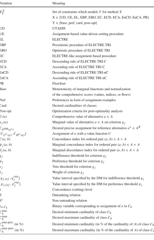
Table 1 Notation
Notation Meaning
EYX Set of constraints which models Y for method X
X∈ {UD,UE,EL,EBP,EBO,EC,ECD,ECA,EnCD,EnCA,PR} Y∈ {base,pref,card,post-opt}
UD UTADIS
UE Assignment-based value-driven sorting procedure
EL ELECTRE
EBP Pessimistic procedure of ELECTRE TRI
EBO Optimistic procedure of ELECTRE TRI
EC ELECTRE-like assignment-based procedure
ECD Descending rule of ELECTRE TRI-C
ECA Ascending rule of ELECTRE TRI-C
EnCD Descending rule of ELECTRE TRI-nC
EnCA Ascending rule of ELECTRE TRI-nC
PR FlowSort
Base Monotonicity of marginal functions and normalization of the comprehensive scores (values, indices, or flows) Pref Preferences in form of assignment examples Card Desired cardinalities of classes
Post-opt Optimization criteria for post-optimality analysis
U(a) Comprehensive value of alternative a∈A uj(a) Marginal value of alternative a∈A on criterion gj
ChDM(a∗) Desired precise assignment for reference alternative a∗∈AR
[CLU(a),CRU(a)] Assignment of a with a value function U
C(a,b) Concordance index for ordered pair(a,b)∈A×A
ψj(a,b) Marginal concordance index for ordered pair(a,b)∈A×A
dj(a,b) Marginal discordance index for ordered pair(a,b)∈A×A
qj Indifference threshold for criterion gj
pj Preference threshold for criterion gj vj Veto threshold for criterion gj
kj Weight of criterion gj
[qj,i n f,qsupj ] Value interval specified by the DM for indifference threshold qj
[pj,i n f,psupj ] Value interval specified by the DM for preference threshold pj
λ Concordance (cutting) level
S Outranking relation
Sc Non-outranking relation
va,Ch Binary variable corresponding to assignment of a to Ch
Chmin Desired minimum cardinality of class Ch
Chmax Desired maximum cardinality of class Ch
Chmin-perc(in %) Desired minimum cardinality (in % of the cardinality of A) of class Ch
Table 1 continued
Notation Meaning
Chmin,l Desired minimum cardinality of union of classes Ch,Ch+1, …, Cl
Chmax,l Desired maximum cardinality of union of classes Ch,Ch+1, …, Cl
a∗j(aj,∗) Alternative a∈A with the best (worst) evaluation on gj
employ in the UTADISGMSmethod [10] general monotone value functions and, additionally, propose to compute necessary assignments which specify the most certain recommendations worked out on the basis of all compatible value functions considered simultaneously. Both methods are interactive in the sense that during the solution process the DM is occasionally required to place some additional reference alternatives into classes, that affects classification of the remaining alternatives as well.
When it comes to an example-based value driven sorting procedure, classes are implic-itly delimited by some assignment examples rather than threshold on a utility scale (see, e.g., [11,17]). Precisely, such a procedure is driven by a value function U and its associated assignment examples. The procedure assigns an alternative a ∈ A to an interval of classes
[CLU(a),CRU(a)], in the following way (note that we assume precise assignment examples):
LU(a)= Max hDM(a∗):U(a∗)≤U(a), a∗∈AR , RU(a)= Mi n hDM(a∗):U(a∗)≥U(a), a∗∈ AR .
In particular, if there is at least one assignment example for each class, then each non-refer-ence alternative can be assigned either to one or two consecutive classes. When using such a procedure, the consistency of a value function U with a set of assignment examples could be modeled in the following way:
U(a∗)≥U(b∗)+ε,
for all a∗,b∗∈AR,such that hDM(a∗) >hDM(b∗). EprefUE
2.2 ELECTRE-like methods
When approaching sorting problems with the use of outranking methods [22], we shall employ a preference model in the form of an outranking relation which becomes true when a concor-dance index is greater than some cutting level. We will also not take into account the veto phe-nomenon. In order to construct an outranking model, we assume that the intra-criterion pref-erence information concerning indiffpref-erence and prefpref-erence thresholds pj ≥qj ≥0,j ∈J , respectively, is given. Note that when comparing two alternatives a,b∈ A on a given cri-terion, the zone between indifference and preference thresholds corresponds to hesitation between opting for indifference and preference. We admit that the DM provides a real inter-val for each threshold, rather than a precise inter-value. We use the following notation to represent these intervals:
– [qj,i n f,qjsup], where qj,i n f and qsupj are, respectively, the least and the greatest value of indifference threshold allowed by the DM,
– [pj,i n f,psupj ], where pj,i n f and psupj are, respectively, the least and the greatest value of preference threshold allowed by the DM.
The concordance index represents the strength of the coalition of criteria being in favor of the statement “a outranks b” (a Sb). It is defined in the following way:
C(a,b)=
m
j=1
ψj(a,b),
where the marginal concordance indicesψj(a,b),j ∈ J , are defined as in [7] and [13], i.e., they are general non-decreasing real-valued functions with clearly distinguished zones of strict and weak preference as well as indifference, and not only piecewise linear or of other arbitrarily chosen shape. We are bounding, however, the area of variation of a mar-ginal concordance index in the zone of weak preference using some extreme linear shapes of this index, which are consistent with the intra-criterion preference information provided by the DM. Moreover, we assume that no criterion is more important than all the other cri-teria jointly. Consequently, the compatible marginal concordance indices are defined by the following set of constraints:
m j=1ψj(a∗j,aj,∗)=1, for all j∈J : (gj(a∗j)=x nj(A) j )and(gj(aj,∗)=x1j)with a∗j,aj,∗∈A, ψj(a∗j,aj,∗)≤0.5, j∈J, for all(a,b,c,d)∈ A×A×A×A, j ∈J : ψj(a,b)≥ψj(c,d) if gj(a)−gj(b) >gj(c)−gj(d), ψj(a,b)=ψj(c,d) if gj(a)−gj(b)=gj(c)−gj(d), for all(a,b)∈A×A, j∈J : ψj(a,b)=0 if gj(a)−gj(b)≤ −psupj , ψj(a,b)≥ε if gj(a)−gj(b) >−pj,i n f, ψj(a,b)=ψj(a∗j,aj,∗) if gj(a)−gj(b)≥ −qj,i n f, ψj(a,b)+ε≤ψj(a∗j,aj,∗) if gj(a)−gj(b) <−qsupj , ψj(a,b)≥ψj(a∗j,aj,∗)· [pj,i n f −(gj(b)−gj(a))]/(pj,i n f −qj,i n f) if −qj,i n f >gj(a)−gj(b) >−pj,i n f, ψj(a,b)≤ψj(a∗j,aj,∗)· [psupj −(gj(b)−gj(a))]/(psupj −q sup j ) if −qsupj >gj(a)−gj(b) >−psupj . ⎫ ⎪ ⎪ ⎪ ⎪ ⎪ ⎪ ⎪ ⎪ ⎪ ⎪ ⎪ ⎪ ⎪ ⎪ ⎪ ⎪ ⎪ ⎪ ⎪ ⎪ ⎪ ⎪ ⎪ ⎪ ⎪ ⎪ ⎬ ⎪ ⎪ ⎪ ⎪ ⎪ ⎪ ⎪ ⎪ ⎪ ⎪ ⎪ ⎪ ⎪ ⎪ ⎪ ⎪ ⎪ ⎪ ⎪ ⎪ ⎪ ⎪ ⎪ ⎪ ⎪ ⎪ ⎭ EELbase
If the compatible concordance indices would be used in a method that takes into account class profiles B = {b0,b1, . . . ,bp}, then in the above formulation one should consider set
A∪B instead of A only. For a more detailed definition and explanation of each constraint, see [7]. Note that the lower and upper bounds for indifference and preference thresholds can be defined by means of non-decreasing functions taking gj(a)as an argument; then, they are denoted by[qj,i n f(a),qsupj (a)]and[pj,i n f(a),psupj (a)]. In particular, these can be affine functions which are used in most ELECTRE methods. Moreover, in case the DM is able to provide preference information about the weights of the criteria kj,j∈J , we may represent the DM’s preference statements in the following way:
– interval weights of the criteria kj, i.e. kj ∈ [kj,∗,k∗j] ⇒ ψj(a∗j,aj,∗) ≥ kj,∗ and ψj(a∗j,aj,∗)≤k∗j,
– pairwise comparisons of the weights of the criteria, e.g., ki ≥ kj ⇒ ψi(ai∗,ai,∗) ≥ ψj(a∗j,aj,∗).
We conclude that a outranks b, if C(a,b)≥λ, whereλ∈ [0.5,1]is a concordance cutting level, and that a does not outrank b (a Scb), otherwise. Knowing whether S is true or not for
an ordered pair of alternatives(a,b) ∈ A×A, one is able to represent situations of weak (Q) or strict (P) preference, indifference (∼), and incomparability (?) among a and b:
a Sb and bSca⇔a Qb or a Pb⇔ab, where = {Q∪P}, a Sb and bSa⇔a∼b, a Scb and bSca⇔a?b. ⎫ ⎪ ⎪ ⎬ ⎪ ⎪ ⎭
The first outranking-based method for multiple criteria sorting problems was ELECTRE TRI [24]. It compares alternatives to some evaluation profiles which are considered as represen-tative fictitious alternatives delimiting the classes from the top and from the bottom. The profiles are denoted by b0,b1, . . . ,bp, with bh,h=1, . . . ,p−1, being the upper profile of class Chand the lower profile of class Ch+1. The method verifies the truth of an outranking relation S between pairs composed of alternatives and class profiles, and exploits this relation to assign each alternative to a specific class, using two assignment procedures. A pessimistic procedure compares a successively to bh, for h =p−1, . . . ,0, and assigns it to class Ch+1, finding the first profile bh, such that a Sbh. Using the terms of the model employed in this paper, a is assigned to Ch, according to the pessimistic procedure, if the following set of constraints is satisfied:
C(a,bt)≥λ, for t=0, . . . ,h−1,
C(a,bt)+ε≤λ, for t=h, . . . ,p−1.
However, since ELECTRE TRI requires that bt dominates bt−1,t=1, . . . ,p, the above set of conditions could be reduced to the following set of constraints:
C(a,bh−1)≥λ,
C(a,bh)+ε≤λ,if h <p.
As far as an optimistic procedure is concerned, it compares a successively to bh,h = 1, . . . ,p, and assigns it to class Ch, such that bh is the first profile for which bh a. As a result, a is assigned to Ch, if the following set of constraints is satisfied:
C(a,bt)≥λ−M·v1(a,bt), C(bt,a)+ε≤λ+M·v2(a,bt), v1(a,bt)+v2(a,bt)≤1, ⎫ ⎬ ⎭ for t =1, . . . ,h−1; if h>1, C(bh,a)≥λ, C(a,bh)+ε≤λ, if h<p, ⎫ ⎪ ⎪ ⎪ ⎪ ⎬ ⎪ ⎪ ⎪ ⎪ ⎭
wherev1(a,bt)andv2(a,bt)are binary variables, which guarantee that either C(a,bt)≥λ or C(bt,a) < λholds for t = 1, . . . ,h−1. Note that although original ELECTRE TRI method does not require the DM to specify assignment examples, the above set of constraints may be used in the ordinal regression approach to model such exemplary assignments in case the DM is able to provide some. Then, such a set of constraints needs to be added for all a∗ ∈ AR with the proviso that h is replaced by hDM(a∗). Let us denote the collective set of constraints obtained in this way by EprefEBP(for a pessimistic procedure) and EprefEBO(for an optimistic procedure).
Specifying the class profiles can be an overwhelming task for a DM. For such decision making situations, there were proposed some outranking methods which require the DM to provide indirect preference information in the form of assignment examples (see, e.g., [6,16,21]). An outranking model is said to be consistent with a set of assignment examples if and only if:
which can be expressed in a equivalent way as:
∀a∗,b∗∈AR, hDM(a∗) >hDM(b∗)⇒b∗Sca∗.
In terms of an outranking model used in this paper, these requirements can be translated into the following set of constraints:
C(a∗,b∗)+ε≤λ, for all (a∗,b∗)∈AR×AR, such that hDM(a∗) <hDM(b∗). E
EC pref
The assignment of the remaining alternatives relies on construction of the model which maintains the desired relations between them and the reference alternatives.
Note that an outranking model based on the concordance index without veto phenomenon is employed in a variety of multiple criteria methods (see, e.g., [5,16]). However, within the proposed framework, we could also model the truth and falsity of the outranking relation in a different way. For example, to avoid the need of specification of comparison thresholds by the DM, we could use a simplified model which is in line with the axiomatic approach of Bouyssou and Marchant [3]. Precisely,ψj(a,b)= ψj(a∗j,aj,∗), if gj(a)≥ gj(b), and ψj(a,b)=0, otherwise. Furthermore, we could take advantage of a more complete model used in ELECTREGKMS[7], and require a Sb to be true if and only if concordance index C(a,b)is not less than a concordance cutting levelλ, and a is not significantly (by more than a veto threshold) worse than b on any criterion, i.e.:
C(a,b)=
m
j=1
ψj(a,b)≥λ and gj(b)−gj(a) < vj, j ∈J,
On the contrary, a does not outrank b, if either concordance index C(a,b)is less than a concordance cutting levelλ, or there is at least one criterion gj for which b is evaluated better than a by more than a veto thresholdvj, i.e.:
C(a,b)= m j=1 ψj(a,b) < λ+M0(a,b) and gj(b)−gj(a)≥vj−M·Mj(a,b), where Mj(a,b)∈ {0,1}, j=0, . . . ,m,and m j=0 Mj(a,b)≤m.
Alternatively, we could refer to the credibility degree used in [21], which is defined as follows: S(a,b)=C(a,b)· [1−dmax(a,b)],
where dmax(a,b)=maxj∈Jdj(a,b), and dj(a,b)is a single-criterion discordance index, which takes a value in the range[0,1], depending on the comparison of the difference gj(b)−gj(a)with the veto thresholdvj (for details, see [21]). In the latter variant, the DM would be required to provide precise values for comparison thresholds.
It is also worth stressing that the approach presented in this paper remains valid for the original definition of the credibility degree presented in the ELECTRE TRI method [19,24]. However, the use of such a model in the context of imprecise or indirect preference informa-tion is limited by the weak efficiency of non-linear mixed integer programming solvers.
In the following sections, the considered sorting methods based on preference model either in the form of value function or outranking relation, will be called UTADIS-like methods or ELECTRE-like methods, respectively.
Table 2 Evaluation table for the
assessment problem of sales managers Alternative g1 g2 g3 Abramov (A) 100 100 44 Chen (C) 85 37 42 Dall (D) 72 69 59 Ellison (E) 13 0 68 Furukawa (F) 0 43 13 Girouille (G) 93 86 31 Hartley (H) 55 23 17 Ivashko (I) 72 23 25 Johnson (J) 32 86 97 Morillo (M) 29 70 12 Naray (N) 41 88 100 Petersson (P) 49 1 0 Stevens (S) 60 50 12 Trainini (T) 15 9 8 Youssef (Y) 2 51 64
Table 3 The allowed ranges of
possible values of indifference and preference thresholds for the assessment problem of sales managers
qj,i n f qsupj pj,i n f psupj
g1 2 4 6 9
g2 1 3 5 7
g3 1 3 4 5
Illustrative example (part 1)
For the purpose of illustration, let us reconsider the problem discussed in [9], which is about evaluating the performance of company’s international sales managers in order to sort them into four classes associated with incentive packages, C={low (LO), lower-middle (LM), upper-middle (UM), high (HI)}. We will refer to it in the following sections to illus-trate different aspects of the proposed framework. We will approach the problem with the UTADIS-like procedure and the ELECTRE-like procedure, both requiring the DM to provide some assignment examples.
Personnel department has considered 15 managers working in different countries. They have taken into consideration three criteria with an increasing direction of preference: sales skills (g1), territory management skills (g2), and customer satisfaction (g3). The evaluations of the alternatives are provided in Table2(the abbreviations of the names will be used to refer to the alternatives in the mathematical constraints).
Let us assume that the DM is able to express the following precise judgments about four sales managers: Chen deserves high (HI) incentive package, Ivashko should receive upper-middle (UM) bonus, and the desired classes for Youssef and Trainini are lower-middle (LM) and low (LO), respectively. In order to get a recommendation using the ELECTRE-like method, the DM has to provide preference information consisting of the intervals of possible values of indifference and preference thresholds (see Table3).
The set of constraints which defines the set of value functions compatible with the pro-vided assignment examples is the following [to save space, we provide only exemplary monotonicity constraints (two for each marginal value function)]:
u1(g1(Y))−u1(g1(F))≥0;. . .;u1(g1(A))−u1(g1(G))≥0; u2(g2(P))−u2(g2(E))≥0;. . .;u2(g2(A))−u2(g2(N))≥0; u3(g3(T))−u3(g3(P))≥0;. . .;u3(g3(N))−u3(g3(J))≥0; u1(g1(F))=0; u2(g2(E))=0; u3(g3(P))=0; u1(g1(A))+u2(g2(A))+u3(g3(N))=1; U(C)≥U(I)+ε; U(I)≥U(Y)+ε; U(Y)≥U(T)+ε. ⎫ ⎪ ⎪ ⎪ ⎪ ⎪ ⎪ ⎬ ⎪ ⎪ ⎪ ⎪ ⎪ ⎪ ⎭
The set of constraints which defines the set of compatible outranking models is the follow-ing [to save space, we provide only exemplary constraints concernfollow-ing the shape of marginal concordance functions (one for each constraint type)]:
ψ1(A,F)+ψ2(A,E)+ψ3(N,P)=1;
ψ1(A,F)≤0.5; ψ2(A,E)≤0.5; ψ3(N,P)≤0.5;
ψ1(A,D)≥ψ1(A,C), since g1(A)−g1(D) >g1(A)−g1(C); ψ1(A,C)≥ψ1(T,F), since g1(A)−g1(C)=g1(T)−g1(F); ψ1(C,A)=0, since g1(C)−g1(A)≤ −p1sup= −9; ψ1(A,C)≥ε, since g1(A)−g1(C) >−p1,i n f = −6; ψ1(A,C)=ψ1(A,F), since g1(A)−g1(C)≥ −q1,i n f = −2; ψ1(C,A)+ε≤ψ1(A,F), since g1(C)−g1(A) <−q1sup = −4; ψ1(H,S)≥ψ1(A,F)·1/4, since −q1,i n f >g1(H)−g1(S) >−p1,i n f; ψ1(H,S)≤ψ1(A,F)·4/5, since −q1sup>g1(H)−g1(S) >−psup1 ; . . . C(T,Y)+ε≤λ; C(T,I)+ε≤λ; C(T,C)+ε≤λ; C(Y,I)+ε≤λ;C(Y,C)+ε≤λ; C(I,C)+ε≤λ. ⎫ ⎪ ⎪ ⎪ ⎪ ⎪ ⎪ ⎪ ⎪ ⎪ ⎪ ⎪ ⎪ ⎪ ⎪ ⎪ ⎪ ⎪ ⎪ ⎪ ⎪ ⎪ ⎪ ⎬ ⎪ ⎪ ⎪ ⎪ ⎪ ⎪ ⎪ ⎪ ⎪ ⎪ ⎪ ⎪ ⎪ ⎪ ⎪ ⎪ ⎪ ⎪ ⎪ ⎪ ⎪ ⎪ ⎭
Provided preference information is consistent, and, consequently, a set of compatible instances of the preference model is not empty.
3 Preference information referring to the desired cardinalities of classes
In this section, we present mathematical models which represent preference information of the DM referring to the desired cardinalities of classes. Note that in all formulations below, M is an auxiliary variable equal to a big positive value,εis a small positive value, andva,Ch is a binary variable associated with assignment of alternative a to class Ch.
Let us first introduce the base model which will be used by different sorting methods. For all these methods, whenever contrary is not explicitly stated, we assume that each alternative a∈ A is to be assigned to exactly one class, i.e., for all a∈A:
p
h=1
va,Ch =1,
and that all exemplary assignments provided by the DM are reproduced, i.e., for all reference alternatives a∗∈ AR:
va∗,C
The constraints specific for each method are the following: – for the UTADIS-like method using class thresholds:
(U D1)U(a)≥bh−1−M·(1−va,Ch), h=1, . . . ,p, for all a∈ A, (U D2)U(a)+ε≤bh+M·(1−va,Ch), h=1, . . . ,p, for all a∈A. E
UD card Constraints(U D1)and(U D2)compare U(a)for all alternatives in A with the lower bh−1and upper bhthresholds of class Ch,h=1, . . . ,p. If a binary variableva,Ch, which is associated with the comparison of a with thresholds delimiting the class Ch, was equal to 0, then the corresponding constraints would always be satisfied, which is equivalent to elimination of these constraints. On the contrary, ifva,Ch was equal to 1, then alternative
a would be assigned to class Ch, because its comprehensive value U(a)satisfies the fol-lowing conditions: bh−1≤U(a) <bh. As a result, U(a)is greater than comprehensive values of all reference alternatives assigned by the DM to any class worse than Ch, and it is smaller than comprehensive values of all reference alternatives assigned by the DM to any class better than Ch.
– for an example-based value driven sorting procedure:
(U E1)U(a)+M·(1−va,Ch)≥U(b)+ε−M·(1−vb,Ch−1),
h=2, . . . ,p, for all a∈ A, for all b∈A\ {a},
(U E2)U(a)+ε−M·(1−va,Ch)≤U(b)+M·(1−vb,Ch+1),
h=1, . . . ,p−1,for all a∈A,for all b∈ A\ {a}.
⎫ ⎪ ⎪ ⎬ ⎪ ⎪ ⎭ EUEcard
Constraints(U E1)and(U E2)make sure that, when assigned to class Ch, the compre-hensive value of alternative a is greater than comprecompre-hensive values of all alternatives (including non-reference ones) assigned by the procedure to class Ch−1, and it is less than comprehensive values of all alternatives assigned to class Ch+1.
If we did not require the final recommendation for each alternative to be a single class assignment, the respective model would be the following:
(U E1) hp=1va,Ch ≥1,
(U E2)U(a)+M·(1−va,Ch)≥U(aC<h)+ε, h=2, . . . ,p, for all a∈A, for all aC<h ∈A
R,such that hDM(a
C<h) <h, (U E3)U(a)+ε−M·(1−va,Ch)≤U(aC>h), h=1, . . . ,p−1,
for all a∈A, for all aC>h ∈AR,such that hDM(aC>h) >h.
⎫ ⎪ ⎪ ⎪ ⎪ ⎬ ⎪ ⎪ ⎪ ⎪ ⎭ EcardUE
The explanation of the constraints is analogous to the explanation given in the previous case with the proviso that we collate comprehensive value of a with comprehensive values of reference alternatives only.
– for the ELECTRE-like method with preference information in the form of assignment examples:
(EC1)C(aC<h,a)+ε≤λ+M·(1−va,Ch), h=2, . . . ,p, for all a∈ A, for all aC<h ∈ AR, such that hDM(aC<h) <h, (EC2)C(a,aC>h)+ε≤λ+M·(1−va,Ch), h=1, . . . ,p−1,
for all a∈ A, for all aC>h ∈ A
R, such that hDM(a C>h) >h. ⎫ ⎪ ⎪ ⎬ ⎪ ⎪ ⎭ EcardEC
Constraints(EC1)and(EC2)guarantee that, when assigned to class Ch, alternative a does not outrank any reference alternative assigned by the DM to a class worse than Ch, and is not outranked by any reference alternative assigned by the DM to a class better than Ch, respectively. Consequently, a is either incomparable to each of these alternatives, or it is preferred to (worse than) reference alternatives assigned by the DM to classes worse (better) than Ch.
– for a pessimistic rule of the ELECTRE-TRI-like method:
(E B P1)C(a,bh−1)≥λ−M·(1−va,Ch), h=1, . . . ,p, for all a∈ A, (E B P2)C(a,bh)+ε≤λ+M·(1−va,Ch)h=1, . . . ,p−1,for all a∈A. E
EBP card Constraints(E B P1)and(E B P2)make sure that, when assigned to class Ch, alternative
a outranks all lower profiles of classes not better than Ch, and does not outrank all lower profiles of classes better than Ch.
– for an optimistic rule of the ELECTRE-TRI-like method: (E B O1)C(bh,a)≥λ−M·(1−va,Ch),
h=1, . . . ,p−1, for all a∈A,
(E B O2)C(a,bh)+ε≤λ+M·(1−va,Ch),
h=1, . . . ,p−1, for all a∈A,
(E B O3)C(a,b<h)+M·v1a,bh ≥λ−M·(1−va,Ch),
h=2, . . . ,p,for all a∈A, for all b<h ∈ {bt,t=1, . . . ,h−1}, (E B O4)C(b<h,a)+ε−M·va2,bh ≤λ+M·(1−va,Ch),
h=2, . . . ,p, for all a∈A, for all b<h ∈ {bt,t=1, . . . ,h−1}, (E B O5) v1a,b h+v 2 a,bh ≤1+M·(1−va,Ch), h=2, . . . ,p, for all a∈A. ⎫ ⎪ ⎪ ⎪ ⎪ ⎪ ⎪ ⎪ ⎪ ⎪ ⎪ ⎪ ⎪ ⎪ ⎪ ⎬ ⎪ ⎪ ⎪ ⎪ ⎪ ⎪ ⎪ ⎪ ⎪ ⎪ ⎪ ⎪ ⎪ ⎪ ⎭ EEBOcard
Constraints(E B O1)and(E B O2)guarantee that all upper profiles of classes not worse than Chare preferred to alternative a which is assigned to class Ch. Further, constraints (E B O3), (E B O4), and(E B O5)make sure that upper profiles of classes worse than Chare not preferred to a (i.e., for all bt,t =1, . . . ,h−1, either btSca or a Sbt, which guarantees that one of the following relations holds: a∼btor a bt or a?bt).
In AppendixA, we present mathematical models representing assignment rules used in ELECTRE-TRI-C [1], ELECTRE-TRI-nC [2] and FlowSort [20] outranking methods. These models can further incorporate the preference information referring to the desired cardinali-ties of classes. This proves generality of the proposed methodology.
Let us pass now to the modeling of the desired cardinalities of classes in terms of con-straints which will be added to the previously defined mathematical models. These concon-straints are the same irrespective of the sorting method under consideration:
– Chshould contain at least Chminand at most Chmaxalternatives, with Chmin≤Chmax: (C L) a∈Ava,Ch ≥Chmin,
(CU) a∈Ava,Ch ≤Chmax.
Note that ifva,Ch was equal to 0, then we relax all conditions which are necessary to assign a to class Ch. On the contrary, ifva,Ch was equal to 1, then a is assigned to class
Ch, since all constraints which are necessary to place a in Ch are satisfied. Constraint (C L)ensures that there are at least Cmin
h alternatives assigned to Ch, whereas constraint (CU)guarantees that there are at most Cmaxh alternatives assigned to Ch. Obviously, we can use either(C L)or(CU)only to model the requirements concerning the lower or upper bound on the cardinality of class Ch, respectively.
– Chshould contain at least Chmin-perc(in %) and at most C max-perc
h (in %) of alternatives,
with Chmin-perc≤Chmax-perc”:
(C L%) a∈Ava,Ch ≥ C min-perc h ·n, (CU %) a∈Ava,Ch ≤ Chmax-perc·n.
If the DM expressed the desired cardinality of class Chin terms of the percentage of the whole set of alternatives A (e.g., 5, 10 %, a quarter, one third, or half of all alternatives), such statement would be modeled analogously to situation when the cardinality is pro-vided explicitly. However, if Chmin-perc(Chmax-perc) of n was not equal to a natural number, we need to guarantee that the smallest (the greatest) number of alternatives which may be assigned to Chis equal toChmin-perc·n(C
max-perc h ·n).
– the range of k contiguous classes Ct,t=h,h+1, . . . ,h+k−1, should contain at least
Chmin,k and at most Cmaxh,k alternatives, with Chmin,k ≤Chmax,k and k≥1: (U C L) ht=+hk−1a∈Ava,Ct ≥Cminh,k, (U CU) ht=+hk−1a∈Ava,Ct ≤Chmax,k .
This type of statement could be used to express the requirements with respect to the cardinality of class union Ch≥(classes not worse than Ch, i.e., a set of the(p−h+1) best classes) and Ch≤(classes not better than Ch, i.e., a set of the h worst classes). Obvi-ously, the statements expressing the cardinality of the union of classes with respect to the percentage of the whole set of alternatives could be modeled analogously to the previous case.
– relative comparisons of cardinalities of different classes, e.g., class Ch should contain
not less alternatives than class Cl, i.e.:
a∈A va,Ch ≥ a∈A va,Cl.
This kind of inequality could also be used to model the requirement that the number of alternatives assigned to each class should be more or less the same, i.e. they should not differ by more than a given number.
Let us denote the set of constraints modeling the statements of the DM referring to the cardinalities of classes by Ecardreq.
Illustrative example (part 2)
For our illustrative example, let us additionally assume that the DM needs to obey some fund-ing limits and, thus, (s)he defines some requirements with respect to the numbers of sales managers who should be assigned to the best and to the worst class. Precisely, the sorting method should assign from 2 to 4 alternatives to class HI, and from 3 to 5 alternatives to class LO. Translating these requirements into mathematical constraints requires the use of binary variableva,Ch for each a∈ A and h∈ H . For example, a binary variablevA,CH I is associated with the assignment of Abramov (A) to class HI.
The constraints which guarantee that all assignment examples and all desired cardinalities of classes are reproduced is the following:
vC,CH I =1; vI,CU M =1; vY,CL M =1; vT,CL O =1; vA,CL O+vA,CL M+vA,CU M+vA,CH I =1;. . .; vY,CL O+vY,CL M+vY,CU M+vY,CH I =1; vA,CL O+vC,CL O + · · · +vT,CL O+vY,CL O ≥3; vA,CL O+vC,CL O + · · · +vT,CL O+vY,CL O ≤5; vA,CH I+vC,CH I + · · · +vT,CH I+vY,CH I ≥2; vA,CH I+vC,CH I + · · · +vT,CH I+vY,CH I ≤4. ⎫ ⎪ ⎪ ⎪ ⎪ ⎪ ⎪ ⎪ ⎪ ⎬ ⎪ ⎪ ⎪ ⎪ ⎪ ⎪ ⎪ ⎪ ⎭
Further, the constraints specific for the UTADIS-like method are the following (to save space, for both UTADIS- and ELECTRE-like methods we provide explicitly only exemplary constraints regarding assignment of Abramov (A) to different classes):
U(A)+M·(1−vA,CL M)≥U(C)+ε−M·(1−vC,CL O); . . .; U(A)+M·(1−vA,CL M)≥U(Y)+ε−M·(1−vY,CL O); U(A)+M·(1−vA,CU M)≥U(C)+ε−M·(1−vC,CL M); . . .; U(A)+M·(1−vA,CU M)≥U(Y)+ε−M·(1−vY,CL M); U(A)+M·(1−vA,CH I)≥U(C)+ε−M·(1−vC,CU M);. . .; U(A)+M·(1−vA,CH I)≥U(Y)+ε−M·(1−vY,CU M); U(A)+ε−M·(1−vA,CL O)≤U(C)+M·(1−vC,CL M); . . .; U(A)+ε−M·(1−vA,CL O)≤U(Y)+M·(1−vY,CL M); U(A)+ε−M·(1−vA,CL M)≤U(C)+M·(1−vC,CU M); . . .; U(A)+ε−M·(1−vA,CL M)≤U(Y)+M·(1−vY,CU M); U(A)+ε−M·(1−vA,CU M)≤U(C)+M·(1−vC,CH I);. . .; U(A)+ε−M·(1−vA,CU M)≤U(Y)+M·(1−vY,CH I). ⎫ ⎪ ⎪ ⎪ ⎪ ⎪ ⎪ ⎪ ⎪ ⎪ ⎪ ⎪ ⎪ ⎪ ⎪ ⎪ ⎪ ⎪ ⎪ ⎬ ⎪ ⎪ ⎪ ⎪ ⎪ ⎪ ⎪ ⎪ ⎪ ⎪ ⎪ ⎪ ⎪ ⎪ ⎪ ⎪ ⎪ ⎪ ⎭
The constraints specific for the ELECTRE-like method are the following: C(A,Y)+ε≤λ+M·(1−vA,CL O); C(A,I)+ε≤λ+M·(1−vA,CL O); C(A,C)+ε≤λ+M·(1−vA,CL O); C(T,A)+ε≤λ+M·(1−vA,CL M); C(A,Y)+ε≤λ+M·(1−vA,CL M); C(A,I)+ε≤λ+M·(1−vA,CL M); C(T,A)+ε≤λ+M·(1−vA,CU M); C(Y,A)+ε≤λ+M·(1−vA,CU M); C(A,I)+ε≤λ+M·(1−vA,CU M); C(T,A)+ε≤λ+M·(1−vA,CH I); C(Y,A)+ε≤λ+M·(1−vA,CH I); C(C,A)+ε≤λ+M·(1−vA,CH I). ⎫ ⎪ ⎪ ⎪ ⎪ ⎪ ⎪ ⎪ ⎪ ⎪ ⎪ ⎪ ⎪ ⎪ ⎪ ⎪ ⎪ ⎪ ⎪ ⎬ ⎪ ⎪ ⎪ ⎪ ⎪ ⎪ ⎪ ⎪ ⎪ ⎪ ⎪ ⎪ ⎪ ⎪ ⎪ ⎪ ⎪ ⎪ ⎭
4 Multiple criteria sorting methods respecting requirements referring to the desired cardinalities of classes
Let us define the set of instances of the preference model compatible with the preference infor-mation provided by the DM for each sorting method under consideration. For the value-driven sorting procedures, a compatible value function satisfies the following set of constraints: – for the UTADIS-like procedure EUDconsisting of EbaseUD,EprefUD,EcardUD, and Ereqcard; – for an example-based procedure EUEconsisting of EbaseUE,EprefUE,EUEcard, and Ecardreq. For the ELECTRE-like procedures, a compatible outranking model is defined by concordance indices C(a,b), concordance cutting levelλ, indifference qj, and preference pj thresholds, and weights kj, for all a,b∈A,j∈J , satisfying the following set of constraints:
– for the ELECTRE-like method with preference information in the form of assignment examples—EECconsisting of: EbaseEL ,EprefEC,EcardEC, and Ecardreq;
– for a pessimistic rule of the ELECTRE-TRI-like method—EE B P consisting of: EbaseEL ,EprefEBP,EcardEBP, and Ecardreq;
– for an optimistic rule of the ELECTRE-TRI-like method—EEBOconsisting of: EbaseEL , EprefEBO,EcardEBO, and Ecardreq.
In order to verify that the set of compatible instances of the preference model (set of value functionsUAR or set of outranking relationsSAR) is not empty, we consider the following mixed integer linear program (MILP):
Maximize:ε, subject to EAR,
where EARis equal to EUDor EUE or EEC or EEBPor EEBO, depending on the sorting method under consideration. Let us denote byε∗the maximal value ofεobtained from the solution of the above MILP problem, i.e.,ε∗=max (ε), subject to EAR. We conclude that the set of compatible instances of the preference model is not empty, if EAR is feasible and ε∗>0.
If the set of compatible instances of the preference model is not empty, there is usu-ally more than one compatible instance. For the UTADIS-like method, a reasonable way of selecting a single value function consists in maximization of the distance between the values of alternatives placed in each class and the respective class thresholds; in this way, one gets as “sharp” discrimination between classes as possible. This requires consideration of the set of constraints EUD, which is obtained by replacing EcardUD in EUDby the following set of constraints, which define the difference between comprehensive values of alternatives and class thresholds, using additional slack variablesε(C), ε∗(Ch), ε∗(Ch), ε∗(a,Ch), and ε∗(a,C h),h=1, . . . ,p, and a∈A: U(a)+ε∗(a,Ch)≥bh−1−M·(1−va,Ch), h=1, . . . ,p, for all a∈A, ε∗(a,Ch)≥ε∗(Ch), h=1, . . . ,p, for all a∈ A, ε∗(Ch)≥ε(C), h=1, . . . ,p, U(a)+ε∗(a,bh)≤bh+M·(1−va,Ch), h=1, . . . ,p, for all a∈A, ε∗(a,C h)≥ε∗(Ch), h=1, . . . ,p, for all a∈ A, ε∗(C h)≥ε(C), h=1, . . . ,p, ε(C)≥0. ⎫ ⎪ ⎪ ⎪ ⎪ ⎪ ⎪ ⎪ ⎪ ⎬ ⎪ ⎪ ⎪ ⎪ ⎪ ⎪ ⎪ ⎪ ⎭ EUDpost-opt
In order to achieve sharp discrimination, we can conduct the following optimizations in a lexicographic order:
– maximization of the minimal distance of the comprehensive values of alternatives from the respective class thresholds, i.e.: Maxi mi ze: ε(C), subject to EUD;
– maximization of the sum of minimal distances of the comprehensive values of alternatives from each class threshold, i.e.: Maxi mi ze: hp=1(ε∗(Ch)+ε∗(Ch))(with the proviso thatε(C)is equal to the optimal value obtained in the previous point);
– maximization of the sum of elementary distances of the comprehensive values of alterna-tives from the corresponding class thresholds, i.e.: Maxi mi ze: a∈Ahp=1(ε∗(a,Ch)+
ε∗(a,C
h))(with the proviso that ε∗(Ch) andε∗(Ch) are equal to the optimal value obtained in the previous point).
Note that for an example-based value-driven sorting procedure, we should maximize the dis-tance between comprehensive values of the alternatives placed in different classes, rather than between the values of alternatives placed in each class and the respective class thresholds.
For the ELECTRE-like methods, we could proceed analogously and emphasize the con-sequences of assigning the alternatives to particular classes, by making the result of the corresponding concordance tests as sharp as possible. Let us present it on the example of the ELECTRE-like method with preference information in the form of assignment examples.
The selection of a single instance of the compatible outranking relation for the ELECTRE-TRI-like methods can be conducted analogously. We will consider the set of constraints EEC, which is obtained by replacing EEC
cardin EECby the following set of constraints with addi-tional slack variablesε(C), ε∗(C<h), ε∗(C>h), ε∗(a,C<h), andε∗(a,C>h),h =1, . . . ,p, and a∈A:
C(aC<h,a)+ε∗(a,C<h)≤λ+M·(1−va,Ch), h=2, . . . ,p, for all a∈A, for all aC<h ∈A
R,such that hDM(a
C<h) <h, ε∗(a,C<h)≥ε∗(C<h), h=2, . . . ,p, for all a∈A
ε∗(C<h)≥ε(C), h=2, . . . ,p,
C(a,aC>h)+ε∗(a,C>h)≤λ+M·(1−va,Ch)h=1, . . . ,p−1, for all a∈A, for all aC.h ∈ A
R, such that hDM(a C>h) >h, ε∗(a,C>h)≥ε∗(C>h), h=1, . . . ,p−1, for all a∈ A, ε∗(C>h)≥ε(C), h=1, . . . ,p−1, ε(C)≥0. ⎫ ⎪ ⎪ ⎪ ⎪ ⎪ ⎪ ⎪ ⎪ ⎪ ⎪ ⎪ ⎪ ⎬ ⎪ ⎪ ⎪ ⎪ ⎪ ⎪ ⎪ ⎪ ⎪ ⎪ ⎪ ⎪ ⎭ Epost-optEC
Then, analogously to the UTADIS-like method, we could first maximizeε(C), then the sum ofε∗(C<h)andε∗(C>h)for h =1, . . . ,p, and finally the sum of elementary differences ε∗(a,C<h)andε∗(a,C>h)for a∈A and h=1, . . . ,p.
Alternatively, as suggested by Köksalan et al. [15], we could try to force alternatives in higher-level classes to outrank alternatives in lower-level classes, and minimize the number of pairs of alternatives for which this requirement is not satisfied. For this reason, we intro-duce new binary variableswa,a∗ andwa∗,a for all a ∈ A\ARand all a∗ ∈ AR. Ifwa,a∗ was equal to 1, then the desired outranking relation between a and a∗would be violated. Consequently, to select an outranking model with the mini number of such violations, we solve the following MILP problem:
Mi ni mi ze: a∈A\AR a∗∈AR wa,a∗+wa∗,a subject to: EEC C(a,aC<h)≥λ−M·(1−va,Ch)−M·wa,aC<h, h=2, . . . ,p, for all a∈ A\AR, for all aC<h ∈A
R, such that hDM(a
C<h) <h
C(aC>h,a)≥λ−M·(1−va,Ch)−M·waC>h,a, h=1, . . . ,p−1, for all a∈ A\AR, for all aC>h ∈A
R, such that hDM(a C>h) >h. ⎫ ⎪ ⎪ ⎪ ⎪ ⎬ ⎪ ⎪ ⎪ ⎪ ⎭ Epost-optEC
Note that instead of choosing any particular instance of the preference model, we could also take into account all compatible instances and determine the set of possible assignments for each alternative a∈ A. To check whether a could be possibly assigned to a class Ch, it is sufficient to assume in the set of constraints EARthatva,Ch is equal to 1, and, subsequently, check whether the resulting set of constraints is feasible. This needs to be done for all a∈ A for each particular class Ch,h =1, . . . ,p. This approach may be particularly useful in the process of incremental specification of assignment examples by the DM. Knowing the set of possible assignments for each alternative, the DM may wish to change the assignment suggested by the method at a current stage of interaction—such a change will be possible when the set of compatible instances of the preference model in the next iteration will not be empty.
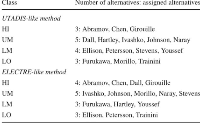
Table 4 The final assignments
for the assessment problem of sales managers
Class Number of alternatives: assigned alternatives
UTADIS-like method
HI 3: Abramov, Chen, Girouille
UM 5: Dall, Hartley, Ivashko, Johnson, Naray LM 4: Ellison, Petersson, Stevens, Youssef LO 3: Furukawa, Morillo, Trainini
ELECTRE-like method
HI 4: Abramov, Chen, Dall, Girouille
UM 5: Ivashko, Johnson, Morillo, Naray, Stevens LM 3: Furukawa, Hartley, Youssef
LO 3: Ellison, Petersson, Trainini
As suggested in [18], in order to support specification of the desired cardinalities of classes Ch,h =1, . . . ,p, one may compute the extreme possible cardinalities given a set of com-patible preference model instances. In the framework of DIS-CARD, this can be achieved by solving the following problem:
Maximize (Minimize): a∈A
va,Ch, subject to EA R
.
Note that thus obtained maximal and minimal cardinalities of each class are certainly, respec-tively, not greater and not less than the corresponding requirements specified by the DM. Obvi-ously, the number of alternatives that are possibly assigned to Chwhen considering the set of compatible model instances, may be, in general, greater than the maximal cardinality of Ch.
Illustrative example (part 3)
In order to choose a single instance which would underly the final recommendation for our illustrative example, for the UTADIS-like method, we maximize the slack variables to obtain as sharp discrimination as possible, whereas for the ELECTRE-like method, we try to force alternatives in higher-level classes to outrank alternatives in lower-level classes and we min-imize the number of violations of this requirement. The corresponding assignments obtained with the use of both sorting methods are presented in Table4.
The assignments of reference alternatives are reproduced and the number of alternatives assigned to the best and to the worst class are within the pre-defined limits. Obviously, the recommendation worked out for some non-reference alternatives is different in case of both methods. In particular, there are seven such alternatives for which the assignment is differ-ent, whereas for the remaining four alternatives the class is the same for UTADIS-like and ELECTRE-like methods. The differences stem from:
– Fundamental differences in assumptions of these methods. Let us remind that the purpose of UTADIS-like methods is to model the decision making situation with an overall value function, and to assign a score to each alternative. Such a score reflects a comprehensive value of the alternative on all criteria considered jointly, and drives the assignment of alternatives to decision classes. The additive value function used in UTADIS-like meth-ods is a compensatory aggregation model admitting that a loss on any criterion can be compensated by a gain on another criterion. When it comes to ELECTRE-like methods, their preference structure is based on a binary outranking relation between particular alter-natives and reference profiles characterizing decision classes. The outranking relation is a
non-compensatory aggregation model. Moreover, it does not assign any numerical score to each alternative. Its exploitation has purely ordinal character.
– Different optimization criteria taken into account when selecting a single compatible instance of the preference model.
– Resulting different priorities assigned to the evaluation criteria in the selected instances of the preference model underlying the final recommendation. Precisely, for the UTA-DIS-like method the maximal difference between comprehensive values of alternatives and class thresholds is equal to 0.142. The greatest share in the comprehensive values is assigned to criterion g1, whereas the least share is assigned to criterion g2. Consequently, sales managers with the best evaluations on g1 (e.g., Abramov, Girouille) are assigned to class HI, whereas alternatives with relatively poor evaluations on g1 are attributed worse incentive packages. When it comes to the ELECTRE-like method, the number of violations of the desired outranking relation between alternatives in higher-level classes and alternatives in lower-level classes is equal to 12 (pairs (Youssed, Ellison), (Ivashko, Furukawa), (Chen, Johnson), etc.). The greatest weights are assigned to g1and g2, which favors alternatives with at least moderately good evaluations on these criteria.
Obviously, the DM may wish to continue the solution process. Precisely, (s)he may add some assignment examples, contradicting the recommendation obtained at the current stage for some non-reference alternatives. Moreover, (s)he may add some requirements with respect to the desired cardinalities of classes UM or LM, or make the requirements which have been already provided for classes HI and LO more precise.
5 Conclusions
In this paper, we introduced a new approach to multiple criteria sorting problems which allows incorporation of preference information concerning the desired cardinalities of clas-ses. The main motivation for this proposal comes from the common use of such requirements in practical situations, the willingness of the DMs to refer to the bounds on the cardinali-ties of classes, and some undesired propercardinali-ties of the recommendation worked out with the use of traditional methods, which do not admit any control of the cardinalities of clas-ses. We proposed some mixed-integer programming models, which allow incorporation of the preference information of this type. Moreover, we have shown that the introduced approach is valid for any type of employed preference model. Precisely, we have proposed some value driven sorting procedures, and some ELECTRE-like methods which are model-ing the DM’s preferences with an outrankmodel-ing relation and require the DM to define the classes with the use of either class profiles, or characteristic alternatives, or assignment examples.
Further research directions include thorough experimental analysis of the introduced approach, and its application to some real world problems e.g., in the field of finance. More-over, this type of preference information may be used in disaggregation procedures which aim to infer precise parameters for the ELECTRE-like methods from imprecise or indirect preferences of the DM.
Acknowledgments The authors would like to thank the anonymous reviewers for their helpful comments and suggestions. The first author wishes to acknowledge financial support from the Poznan University of Technology, grant no. 91-516/DS-MLODA KADRA.
Open Access This article is distributed under the terms of the Creative Commons Attribution License which permits any use, distribution, and reproduction in any medium, provided the original author(s) and the source are credited.