Limited Memory Solution of Complementarity Problems arising in Video Games

Laboratoire d’Arithmétique, Calcul formel et d’Optimisation

UMR CNRS 6090

Limited Memory Solution of Complementarity Problems

arising in Video Games

Michael C. Ferris

Andrew J. Wathen

Paul Armand

Rapport de recherche n° 2004-01

Déposé le 15 avril 2004

Limited Memory Solution of Complementarity

Problems arising in Video Games

∗

Michael C. Ferris

Andrew J. Wathen

Paul Armand

April 7, 2004

Abstract

We describe the solution of a complementarity problem with lim-ited memory resources. The problem arises from physical simulations occurring within video games. The motivating problem is outlined, along with a simple interior point approach for its solution. Various linear algebra issuesc arising in the implementation are explored, in-cluding preconditioning, ordering and a number of ways of solving an equivalent augmented system. Alternative approaches are briefly sur-veyed, and some recommendations for solving these types of problems are given.

1

Introduction

This paper describes the solution of a problem arising in the application of complementarity for physical simulations that occur within video games.

∗_{This material is based on research partially supported by the Smith Institute, EPSRC}

Grant GR/M59044, the National Science Foundation Grant CCR-9972372, the Air Force Office of Scientific Research Grant F49620-01-1-0040, the Guggenheim Foundation, and the Centre National de la Recherche Scientifique (UMR 6090).

†_{Oxford University Computing Laboratory, Wolfson Building, Parks Road, Oxford,}

OX1 3QD Permanent address: Computer Sciences Department, University of Wisconsin, 1210 West Dayton Street, Madison, Wisconsin 53706, USA

‡_{Oxford University Computing Laboratory, Wolfson Building, Parks Road, Oxford,}

OX1 3QD

§_{Laboratoire d’Arithm´etique, de Calcul formel et d’Optimisation, Universit´e de}

The size of the problems is typically not very large, ranging from around 20 variables to a current limit of around 400 variables. The computational time available to solve each instance of the problem is limited by the frame rate of the simulation, and the memory allowed to solve each problem is severely restricted by the hardware available on many of the existing game (console) platforms. The typical time frame is of the order of milliseconds, while the amount of fast RAM available is 4-16K. A further important feature of the solution technique is that worst case behavior is very important - if large spikes in computation occur this can lead to loss of frames and jumpy screen animations.

While these problems are clearly not large scale, the limited memory re-quirement means that techniques normally associated with large scale prob-lems are pertinent. In particular, limited memory methods and conjugate gradient techniques would appear to be applicable.

We now describe some mathematical background on the problem. To handle collisions in physical simulation, it is normally necessary to solve Lin-ear Complementarity Problems (LCP’s) very efficiently. While more general formulations are typically of interest, the form of the LCP considered here is a bound constrained convex quadratic program

min{1

2x

T

Ax+v0Tx:l≤x≤h}.˜

Here, x is the vector to be found, l, ˜h and v0 are given vectors, the bounds

hold componentwise, and A is a symmetric positive semidefinite matrix of

the formA = JM−1

JT _{+D. The matrix A is not computed explicitly, but}

is given by J, M−1

and D. Here M = diag(M1, . . . , Mk) is block diagonal

and each Mi = diag(mi, mi, mi, Ii) is 6×6 with mi and Ii being the mass

and inertia tensor for the ith physical body. In fact, x is the vector of the

impulses at each physical contact,JT_{xis the vector of the impulses applied to}

the bodies,M−1_JT_{xis the vector of velocity changes of the bodies,JM}−1_JT_x

is the vector of relative velocity changes at the physical contacts, and (if we

ignoreD)Ax+v0 is the vector of relative velocities at the physical contacts.

The matrix J is sparse and represents collisions. If bodies i and j are

capable of colliding then J has a set of rows with nonzero entries only for

those bodies; thus it has a (collisions×bodies) block structure.

The matrix D is diagonal with small positive or zero diagonal elements.

Physically, a positive element would correspond to a small springiness in the constraints, but they are not put in to represent a physical effect. They are

sometimes added to makeApositive definite and guarantee uniqueness inx.

Note that ifA is only semidefinite then Ax+v0 will still be unique, even if

xis not.

We have around 1800 test problems from the application each of which is a convex quadratic optimization with simple bound constraints. They are set up as two suites of problems, one labelled “ball” and the other labelled “topple”. While the original problem description specifies bounds on all the

variables, it was decided to treat any bounds with magnitude over 1020

as infinite. The resulting problems then have some doubly bounded variables, some singly bounded variables and some free variables.

The remainder of this paper is organized as follows. In Section 2 we describe a simple interior point approach to solving the problem and show this to be effective in terms of iteration count on the problems at hand. Sec-tion 3 explores the linear algebra issues that arise in an implementaSec-tion of the interior point approach for this application. In particular, we investigate pre-conditioning, ordering and various ways of solving an equivalent augmented system. Section 4 briefly surveys other approaches that were considered and discusses the pros and cons of them compared to the interior point approach. The paper concludes with some recommendations for solving these types of problems and indicates some thoughts for future research.

2

Interior Point Method

For computational ease, the problems were transformed by a simple linear transformation so that doubly bounded variables lie between 0 and a finite upper bound and singly bounded variables are simply nonnegative. Such changes clearly do not affect the convexity properties of the objective function

and result in some simple shifts coupled with a multiplication by −1 of the

rows and columns ofA(or equivalently the rows ofJ) corresponding to singly

upper bounded variables. The resulting problem is thus:

min{1 2x T_Hx+qT_x:x∈ B} where B={x: 0≤xB ≤u,0≤xL, xFfree}.

Introducing multipliers sB, sL and ξ for the bound constraints, the first

sufficient and can be written g:=Hx+q−   sB−ξ sL 0   = 0 0≤xB ⊥ sB ≥0 0≤xL ⊥ sL ≥0 0≤u−xB ⊥ ξ ≥0

where the perp notation means that in addition to the nonnegative bounds, primal and dual variables are orthogonal.

We apply the Primal-Dual Framework for LCP to this problem (see [17], pp. 158–160). The critical system of linear equations (using the standard capitalization notation) that must be solved at each iteration is:

        HBB HBL HBF −I I HLB HLL HLF −I HF B HF L HF F SB XB SL XL −E U −XB                 ∆xB ∆xL ∆xF ∆sB ∆sL ∆ξ         =−Φ (1) where Φ =     g XBsB−σµe XLsL−σµe (U−XB)ξ−σµe     with σ ∈[0,1] and µ= x T BsB+xTLsL+ (u−xB)Tξ kLk+ 2kBk .

We first eliminate ∆sB, ∆sL and ∆ξ from this system to recover the

following problem: (H +θ)∆x= −r (2) where θ= diag(X−1 B sB+ (U−XB) −1 ξ, X−1 L sL,0F) and r=Hx+q−σµθe.

Once this system is solved, we can recover all the required values using back substitution in (1).

Some points of note. We choose σ = 0.1 for all our tests and initialize

the method (for the translated problem) at a point where xi = 1, i ∈ L,

xi =ui/2, i∈ B and xi = 0, i∈ F. The dual variables are set to

si=

0.1 + max{0, Hi,·x+qi} i∈ B,

max{0.1, Hi,·x+qi} i∈ L

and ξi =si−(Hi,·x+qi), i∈ B.

We use two stepsizes, for primal and dual variables, each one been computed by means of the fraction to the boundary rule with 0.9995 as parameter value. We terminate the interior point method when

µ ≤10−8

and kgk ≤(1 +kqk)10−6

.

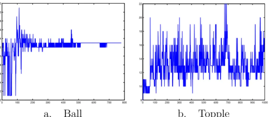
We show on our two suites of test problems that the interior point method is an effective solution approach. Figure 1 shows the number of interior point iterations in each of the problem classes.

0 100 200 300 400 500 600 700 800 0 2 4 6 8 10 12 14 16 18 20 22 0 100 200 300 400 500 600 700 800 900 1000 8 10 12 14 16 18 20 22 a. Ball b. Topple

Figure 1: Interior Point Iterations per Problem: the problems are arbitrarily numbered along the horizontal axis.

While there is some variation over the suite of problems, the number of iterations is bounded above by 22 over all test problems and the vast majority of the solutions occur in no more than 20 iterations of the interior point method. This approach appears very promising provided that we can solve the linear systems within the time and space constraints imposed by the application.

3

Linear Algebra

We investigate the solution of the system (2), which we will refer to as the pri-mal system, using an iterative method. Symmetry and positive (semi-)

def-initeness allow us to use preconditioned conjugate gradients (PCG) to solve (2). The work involved in an iteration of this method is one matrix×vector multiplication plus 5 vector operations (3 vector updates and 2 dot prod-ucts) and 3 additional vectors require storage. The key issue is to determine

an effective preconditioner forH +θ so that the number of linear iterations

needed is small, but little additional memory is required. Note that H has

the form ˜JM−1_J˜T_{+D, where ˜J incorporates the change of signs on the rows}

corresponding to upper bounded variables.

We use the default convergence tolerance of a reduction in Euclidean

norm of the residual in the linear system by 10−6

in all runs of the standard Matlab conjugate gradient code. Despite the relatively small dimension of the linear systems, the conjugate gradient method without preconditioning fails to converge on some of the resulting systems. This is even the case if we relax the convergence tolerance. Given that termination in exact arithmetic

should occur in at mostn steps, this indicates the poor conditioning of some

of the linear systems. Thus we only report results for PCG, and only choose options for which the method achieves the above tolerance. This results in an (almost) identical sequence of iterations of the interior point method.

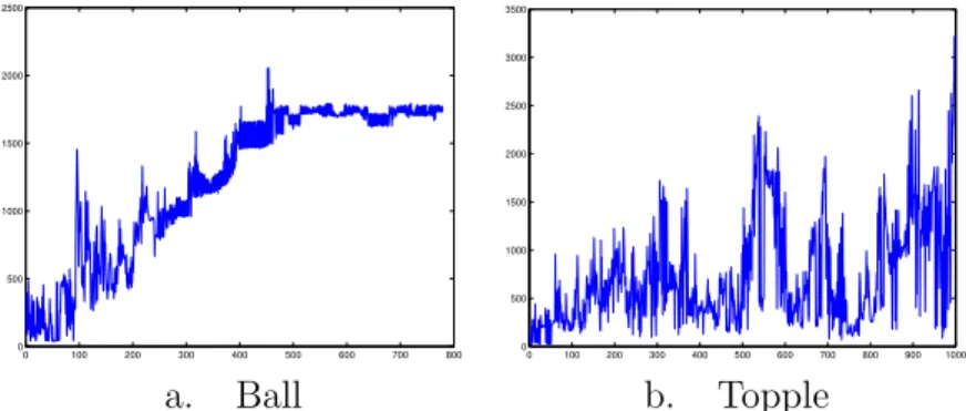
The first preconditioner is the simple diagonal preconditionerθ+ diag(H)

as suggested by [3]. Figure 2 shows that all the resulting problems are then solved, each graph indicating the total number of iterations (matrix-vector products) per problem to solve all the systems generated by the interior point method on each problem class. We experimented with the different

0 100 200 300 400 500 600 700 800 0 500 1000 1500 2000 2500 0 100 200 300 400 500 600 700 800 900 1000 0 500 1000 1500 2000 2500 3000 3500 a. Ball b. Topple

Figure 2: Total conjugate gradient iterations per problem when solving (2)

with preconditioner diag(H) +θ.

diagonal preconditioner θ+ diag(P

off diagonal entries inH, but the results are not as good as those of Figure 2. While additional memory requirements are small, the numbers of matrix-vector products is considered unacceptable for the application.

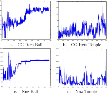
There is evidently significant non-local coupling than can not be ac-counted for by these simple diagonal scalings. We therefore resort to a more sophisticated preconditioner, namely an incomplete Cholesky factorization with a drop tolerance (see for example [16]). Figure 3 shows the number of

0 100 200 300 400 500 600 700 800 0 10 20 30 40 50 60 70 80 0 100 200 300 400 500 600 700 800 900 1000 20 40 60 80 100 120 140

a. CG Iters Ball b. CG Iters Topple

0 100 200 300 400 500 600 700 800 200 400 600 800 1000 1200 1400 1600 1800 2000 0 100 200 300 400 500 600 700 800 900 1000 0 1000 2000 3000 4000 5000 6000 c. Nnz Ball d. Nnz Topple

Figure 3: Total conjugate gradient iterations and number of nonzeros (nnz) in factor per problem when solving (2) with an incomplete Cholesky

factor-ization preconditioner (drop tolerance of 10−4_).

conjugate gradient iterations and the number of nonzeros in the incomplete

Cholesky factor (with drop tolerance 10−4_{) that are required to solve each}

problem using the primal system. Increasing the drop tolerance led to signifi-cant increases in the number of conjugate gradient iterations and was deemed unacceptable. It is clear that the number of conjugate gradient iterations is decreased to a very reasonable number using this approach, but that the size of the factor is too large for the application. Note that the results for the

“topple” problem are particularly bad for this approach. We therefore in-vestigate alternative linear systems in order to generate preconditioners with smaller memory requirements.

3.1

Dual System

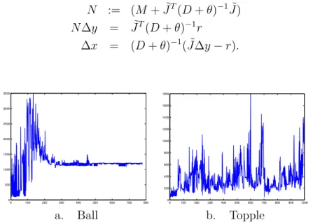
Alternative approaches for solving (2) stem from the equivalent augmented system: M J˜T ˜ J −D−θ ∆y ∆x = 0 r .

This symmetric and indefinite system might be preconditioned using for ex-ample the results of [10] and [14], but without making further assumptions, no effective technique of either type was found in this case. However, just as the original system (2) (the primal system) results from an elimination of ∆y using the first equation, an alternative is to use the dual system where we

first eliminate ∆x using the second equation, then solve for ∆y and finally

use back substitution to calculate ∆x:

N := (M+ ˜JT(D+θ)−1J˜) N∆y = J˜T_(D+θ)−1 r (3) ∆x = (D+θ)−1 ( ˜J∆y−r). 0 100 200 300 400 500 600 700 800 0 500 1000 1500 2000 2500 3000 3500 0 100 200 300 400 500 600 700 800 900 1000 0 200 400 600 800 1000 1200 1400 1600 1800 a. Ball b. Topple

Figure 4: Total conjugate gradient iterations per problem when solving (3)

with preconditioner diag(N).

and diag(P

j|N·j|). The results for the first are given in Figure 4, and remain

very similar for the second (which are not shown).

Figure 5 shows the number of conjugate gradient iterations and the num-ber of nonzero entries in the incomplete Cholesky factor when applied to the system (3). The first point to note is that both of these are reduced on the “topple” problem as compared to the results of Figure 3. This is essentially due to the fact that on these problems the size of the dual system is smaller than that of the primal system. The results for the “ball” problem are less conclusive and show the worse case of both iteration count and number of nonzeros is increased when using the dual approach.

0 100 200 300 400 500 600 700 800 10 20 30 40 50 60 70 80 90 100 110 0 100 200 300 400 500 600 700 800 900 1000 0 10 20 30 40 50 60 70

a. CG Iters Ball b. CG Iters Topple

0 100 200 300 400 500 600 700 800 0 500 1000 1500 2000 2500 3000 0 100 200 300 400 500 600 700 800 900 1000 0 200 400 600 800 1000 1200 1400 a. Nnz Ball b. Nnz Topple

Figure 5: Total conjugate gradient iterations and number of nonzeros (nnz) in factor per problem when solving (3) with an incomplete Cholesky

factor-ization preconditioner (drop tolerance of 10−4_).

This suggests using an approach that switches between the two systems depending on known problem characteristics. We recall that for all the

“top-ple” problemsJ has more rows than columns so that the dual system will be

˜

J are not known, we choose to solve the dual system if 1.2rows( ˜J)≥cols( ˜J).

This is an empirical choice based on the number of nonzeros in the resulting (primal or dual) linear system.

0 100 200 300 400 500 600 700 800 0 20 40 60 80 100 120 0 100 200 300 400 500 600 700 800 900 1000 0 10 20 30 40 50 60 70 a. Ball b. Topple

Figure 6: Total Conjugate Gradient Iterations using both primal and dual systems with an incomplete Cholesky factorization with drop tolerance of

10−4_.

Using this heuristic switching mechanism, the number of conjugate gra-dient iterations remains at a reasonable number as shown in Figure 6. Note that the “topple” problem is always solved using the dual approach, but the “ball” problem switches between the two systems.

3.2

Orderings and Drop Tolerances

If we choose to perform an incomplete factorization then we require the incomplete factors to be reasonably sparse. The storage required for an

incomplete Cholesky factorization with drop tolerance of 10−4

is shown in Figure 3 (c) and (d) and Figure 5 (c) and (d). Ideally, we would like to limit the amount of storage that is available to the preconditioner to 1000 double precision entries and neither approach achieves this goal.

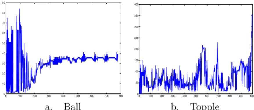
We have investigated ordering the systems at hand to reduce the size of these factors. We found the use of a symmetric reverse Cuthill McKee ordering to be helpful in this respect. If we perform a symmetric reverse

Cuthill McKee ordering ofH+θ or N beforehand (and solve the permuted

problem explicitly), the size of preconditioners generated is shown in Figure 7. Note that the maximum number of PCG iterations required to solve the problem (over all problems in the respective set) using these preconditioners is given in the caption as cgmax.

0 100 200 300 400 500 600 700 800 0 100 200 300 400 500 600 700 800 900 0 100 200 300 400 500 600 700 800 900 1000 0 100 200 300 400 500 600 700 800 900

a. Ball (cgmax = 89) b. Topple (cgmax = 60)

Figure 7: Number of nonzeros in Cholesky factor, using symrcm ordering, a

drop tolerance of 10−4 _{and primal/dual switching.}

However, it should be noted that while the effects of drop tolerances are dramatic in the number of conjugate gradient iterations required, their effect on the number of nonzeros in the factors is somewhat limited. We show two extremes as Figure 8 and Figure 9.

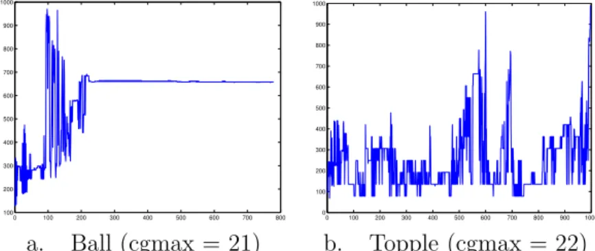
0 100 200 300 400 500 600 700 800 100 200 300 400 500 600 700 800 900 1000 0 100 200 300 400 500 600 700 800 900 1000 0 100 200 300 400 500 600 700 800 900 1000

a. Ball (cgmax = 21) b. Topple (cgmax = 22)

Figure 8: Number of nonzeros in Cholesky factor, using symrcm ordering, a drop tolerance of 0 and primal/dual switching.

Note that only one ordering needs to be carried out, but that an incom-plete factorization must be formed at every iteration of the interior point method. Since the number of interior point iterations and the number of conjugate gradient iterations remains (small and) unchanged, we believe that preconditioning with a very small drop tolerance is an efficient and effective way to solve the problem at hand.

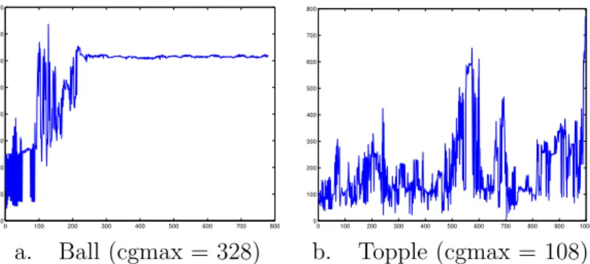
0 100 200 300 400 500 600 700 800 0 100 200 300 400 500 600 700 800 0 100 200 300 400 500 600 700 800 900 1000 0 100 200 300 400 500 600 700 800

a. Ball (cgmax = 328) b. Topple (cgmax = 108)

Figure 9: Number of nonzeros in Cholesky factor, using symrcm ordering, a

drop tolerance of 10−3 _{and primal/dual switching.}

However, while this has proven effective in other applications, it just served to dramatically increase the number of conjugate gradient iterations required in this application.

3.3

Effect of

_D

In both application examples, the matrix D has positive entries, ensuring

that the problem at hand has a unique solution. We carried out a limited

number of experiments where we setD= 0. Since in many cases the matrix

J is quite rank-deficient, this can lead to substantial difficulties in our dual

approach.

However, subject to the following caveats, all problems were solved by our approach. The first caveat is that in the dual approach, it may no longer

be possible to form (3) since D+θ may no longer be invertible. To protect

against this, whenever we solve (2) by first transforming it to (3), we perturb

D+θ to force every entry to be at least 10−8

. The second caveat is that the resulting linear system (3) is very hard to solve and requires an exact factor. For even very small values of the drop tolerance the PCG method failed.

Thus to gain robustness in the method, we suggest using the adaptive pri-mal/dual approach (possibly with very small perturbations), combined with a symmetric reverse Cuthill McKee ordering and solution using exact factor-ization. While it is possible (particularly in the primal system) to employ a drop tolerance in an incomplete Cholesky factorization preconditioner, the gain in terms of memory is very small compared to the increase in conjugate gradient iterations.

4

Other Approaches

We experimented with several other approaches to determine their applica-bility, including OOQP, PATH, SEMI, LBFGS and SPG. The OOQP code did not solve all the problems in the suite so we have not reported results for that code here; however, we note that in the cases successfully solved, the number of interior point iterations used by OOQP was very similar to the code we outlined above.

4.1

PATH and SEMI

We configured the PATH solver [7, 9] to act as a modified Lemke code (using

a regular start instead of a ray start) with termination criteria of 10−4

. Note that each iteration corresponds to a pivot, implementable by a rank-1 update. While the use of a crash procedure [8] does reduce the number of pivots required to solve the problem, we have not reported these results here since we attempted to reduce the overall complexity of the approach.

0 100 200 300 400 500 600 700 800 0 10 20 30 40 50 60 70 80 90 0 100 200 300 400 500 600 700 800 900 1000 0 50 100 150 200 250 300 350 400 a. Ball b. Topple

Figure 10: PATH iterations (using regular start, no crashing).

The iterations required by this approach are quite small, although for the larger test problems in the “topple” suite it increases to nearly 400. This approach could be implemented using the problem specific linear algebra techniques outlined in Section 3. We believe however, the method of Sec-tion 2 will perform better on this applicaSec-tion due to the small fluctuaSec-tion in iteration count in the context of the interior point method.

The semismooth approach described in [13] is similar to the interior point approach that was outlined in Section 2 in that it generates a small number

of linear systems to solve, except that it typically destroys the symmetry

properties ofH. We used an option file that configured the code to carry out

monotone linesearches without a crash procedure and using a Fischer merit function, as these options greatly improved the performance of the code on these problems. The implementation uses an incomplete LU factorization preconditioner to the LSQR iterative solver [15], which by default has a very small drop tolerance. We present the results (with termination criterion of

10−4

) as Figure 11. While the iteration count is very impressive, the number

0 100 200 300 400 500 600 700 800 0 5 10 15 0 100 200 300 400 500 600 700 800 900 1000 0 5 10 15 20 25 30 a. Ball b. Topple

Figure 11: SEMI iterations.

of nonzeros in the LU factors approaches 14,000 even when the Markovitz

ordering is used. It remains a topic for future research to determine if iterative techniques, more specialized reformulations or other orderings can reduce this memory requirement to an acceptable level. A (predictor-corrector) smoothing method implemented within Matlab performs very similarly to the SEMI code.

An advantage of the techniques of this section over the other ones outlined in this paper is that they would perform just as well on convex LCP’s that are not derived directly as the optimality conditions of a convex quadratic optimization problem.

4.2

LBFGS

The limited memory BFGS method [18] appears to be ideally suited to this

application. This code has a limited memory requirement of 2mn + 4∗

n+ 12∗m2

+ 12mwhere mis the memory size of the problem and n is the

suite of test problems giving rise to the iteration counts of the method shown

in Figures 12, 13 and 14. We used the medium accuracy termination

0 100 200 300 400 500 600 700 800 0 200 400 600 800 1000 1200 1400 0 100 200 300 400 500 600 700 800 900 1000 0 100 200 300 400 500 600 a. Ball b. Topple

Figure 12: LBFGS iterations with m= 3.

0 100 200 300 400 500 600 700 800 0 100 200 300 400 500 600 700 800 900 1000 0 100 200 300 400 500 600 700 800 900 1000 0 100 200 300 400 500 600 a. Ball b. Topple

Figure 13: LBFGS iterations with m= 5.

requirements suggested by the authors of the code, and experimented with

3 values of the parameter m. Note that each iteration approximately solves

a model problem determined by the current limited memory approximation

of the Hessian matrixH.

Clearly, these results show that the benefit of m > 3 is not substantial

in terms of iteration count. Furthermore, the amount of memory required

when m = 3 is much smaller, and is therefore preferred. However, even in

this case, the method takes over 6n additional memory, and is thus more

memory intensive that the problem specific approaches outlined above. However, as a general purpose approach to these problems this technique

0 100 200 300 400 500 600 700 800 0 100 200 300 400 500 600 700 800 900 0 100 200 300 400 500 600 700 800 900 1000 0 50 100 150 200 250 300 350 400 450 500 a. Ball b. Topple

Figure 14: LBFGS iterations with m= 10.

explicitly but uses reverse communication to request objective function and

gradient evaluations. Thus, H does not need to be formed, it can be

ap-plied using J, M−1

and D. Furthermore, the memory required is known in

advance and is not affected by changes in density of J. However, the cost

of this method is the number of iterations that are needed - the method

of-ten requires more than 1000 iterations with m= 3 and more than 500 with

m= 10.

4.3

LBFGS preconditioning

Limited memory BFGS updates can also be used to compute a preconditioner for the conjugate gradient method [12]. The method is designed for solving a sequence of slowly varying linear systems. It uses information from the resolution of the current linear system to build an LBFGS approximation matrix as a preconditioner for the next linear system. The benefits of this approach are the same as the LBFGS algorithm, that is, low memory storage,

an amount of memory known in advance and a Hessian matrix H that does

not need to be formed but can simply be applied.

We experimented with a slightly different approach than the one described

by [12]. Since the matrices of the linear systems are of the formH+θ, where

θ is diagonal and is the only term varying during the interior point

itera-tions, we perform an LBFGS approximation of H, say M, and use M +θ

as preconditioner. Formulas and the algorithm for the computation of the

matrix-vector products (M+θ)−1_{v are obtained from a compact}

representa-tion ofM [6] combined with the Sherman-Morrison-Woodbury formula (see

[1]). The memory storage requirement is of 2n(m+ 1) +O(m2

Problem System m= 0 m= 4 m= 8

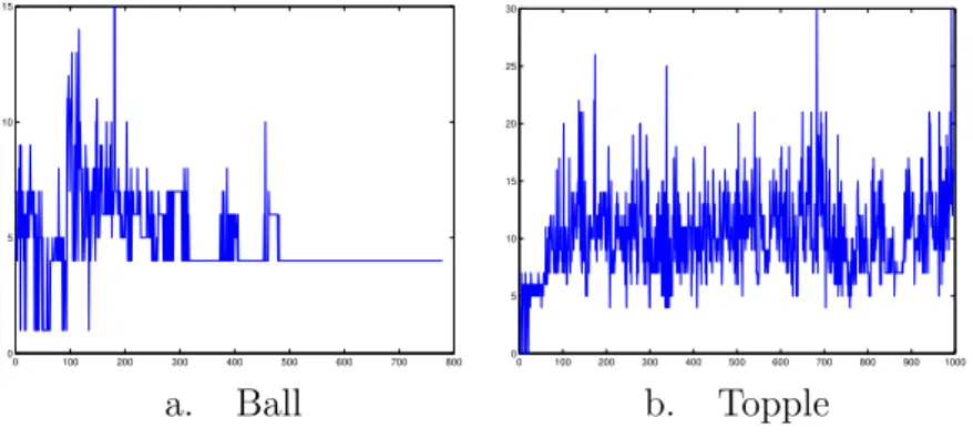
Ball (2) 1225/2055 1047/1728 887/1447

(3) 1243/3485 1147/3474 1013/3310

Topple (2) 727/3225 697/2994 651/2724

(3) 365/1784 317/1625 267/1474

Table 1: mean/max number of conjugate gradient iterations when solving

(2) and (3) with the LBFGS preconditioner.

is the number of vector pairs of length n kept in memory. The choice of

the vector pairs at one iteration is carried out using the SAMPLE algorithm described by [12].

Table 1 shows the mean and maximum numbers of conjugate gradient iterations that are required to solve primal (2) and dual systems (3) for each

class of problems. The parameter m indicates the number of vectors pairs

kept in memory. The value m = 0 corresponds to the solution with the

diagonal preconditioners diag(H) +θ (Figure 2) and diag(N) (Figure 4). We

observed a linear decrease of the number of conjugate gradient iterations for

increasing values of m, but the counterpart is that the computational cost

increases at the same time in a greater proportion.

4.4

SPG

SPG [5] implements a gradient projection method combined with a nonmono-tone line search. It is derived from the Barzilai-Borwein algorithm [2] and is globally convergent for the minimization of a nonlinear differentiable func-tion over a convex set [4]. SPG is particularly well suited to our applicafunc-tion because it needs only to store two gradient vectors and the projected direc-tion of line search, moreover the inner cost of one iteradirec-tion is nearly reduced to the computation of two scalar products.

We use the Fortran 77 code supplied by the authors with the default parameters settings, except that we set the maximum number of function

evaluations to 15000 and the stopping tolerances to 10−4

. Figure 15 shows the total number of function evaluations to solve both problem suites.

SPG is a pure gradient algorithm, and so we observed that a great num-ber of iterations are needed to obtain a sufficiently accurate solution. We observed that the number of function evaluations is greater than 15000 for 23 problems (small circles on Figure 15). These values are prohibitive for

this application. 0 100 200 300 400 500 600 700 800 0 5000 10000 15000 0 100 200 300 400 500 600 700 800 900 1000 0 5000 10000 15000 a. Ball b. Topple

Figure 15: Total function evaluations per problem with SPG.

Another possibility is to use the TRON code [11] that implements a trun-cated Newton approach for this problem with linear systems solved by pre-conditioned conjugate gradients using a limited memory incomplete Cholesky factorization. This has not yet been applied to our test set. Obviously, both these techniques are confined to the optimization framework that we have considered here and seem non-trivial to generalize to the complementarity setting. However, when direct methods are applied to solve (2) or (3), the

symmetry of the underlying systems is no longer as crucial - in fact LU

decomposition can be used in place of Cholesky factorization.

5

Conclusions

This paper has provided a case study of the solution of a particular suite of test problems arising from physical simulations in the video game industry. The paper has proposed an interior point method for solution and has inves-tigated the use of iterative methods to solve the systems of linear equations that arise. Several other codes (PATH, SEMI, L-BFGS-B, SPG) also pro-cess all the models at hand, but are considered inferior to the interior point approach for a variety of reasons.

The interior point approach is theoretically guaranteed to process prob-lems of the type described here and in practice takes very few iterations (linear solves) to generate accurate solutions. The method is easily general-izable to unsymmetric complementarity problems, relying on corresponding changes to the methods needed to solve the resulting linear systems.

We have proposed a primal/dual switching mechanism for solving the underlying linear systems in our method as a means to reduce memory re-quirements. This, coupled with a symmetric reverse Cuthill McKee ordering, allows all the systems to be solved with preconditioner memory requirements of less than 1000 double precision entries. The preconditioner recommended is an incomplete Cholesky factorization with very low drop tolerance. It is interesting to note that in many cases the nonzeros in the preconditioner are

fewer than the nonzeros in the matrixJ.

Unfortunately, the benefits of this preconditioner when coupled with the other features of our solution approach are limited, and direct solution does not take much more memory than the preconditioner, and can lead to more robustness on problems that are not strongly convex. In both cases, we acknowledge the potential drawback of needing to form the matrix used in (2) or (3) in order that the (incomplete) factorization can be carried out.

We believe that the use of iterative methods within the context of in-terior point methods remains a topic of future research. Newly developed codes such as GALAHAD and KNITRO for (quadratic and) nonlinear pro-gramming already incorporate conjugate gradient techniques for subproblem solution in large scale settings.

Limited memory solution of complementarity problems remains an open area for general problems. This paper has shown it to be difficult to use iterative linear equation solvers in the context of convex quadratic programs with simple bounds. Complementarity problems are considered more difficult than these problems for iterative solvers since they generate unsymmetric systems. We remain hopeful that careful study of particular applications, coupled with a more complete understanding of the interplay between theory and implementation will lead to advances in this area.

References

[1] P. Armand and P. S´egalat. A limited memory algorithm for inequal-ity constrained minmization. Technical Report 2003-08, Universinequal-ity of Limoges (France), 2003.

[2] J. Barzilai and J. M. Borwein. Two-point step size gradient methods.

[3] L. Bergamaschi, J. Gondzio, and G. Zilli. Preconditioning indefinite

systems in interior point methods for optimization. Computational

Op-timization and Applications, forthcoming, 2004.

[4] E. G. Birgin, J. M. Mart´ınez and M.Raydan. Nonmonotone spectral

pro-jected gradient methods on convex sets. SIAM Journal on Optimization,

10:1196–1211, 2000.

[5] E. G. Birgin, J. M. Martinez, and M. Raydan. Algorithm 813: Spg

– software for convex-constrained optimization. ACM Transactions on

Mathematical Software, 27:340–349, 2001.

[6] R. H. Byrd, J. Nocedal, and R. B. Schnabel. Representations of

quasi-Newton matrices and their use in limited memory methods.

Mathemat-ical Programming, 63:129–156, 1994.

[7] S. P. Dirkse and M. C. Ferris. The PATH solver: A non-monotone

stabilization scheme for mixed complementarity problems.Optimization

Methods and Software, 5:123–156, 1995.

[8] S. P. Dirkse and M. C. Ferris. Crash techniques for large-scale

com-plementarity problems. In M. C. Ferris and J. S. Pang, editors,

Com-plementarity and Variational Problems: State of the Art, pages 40–61, Philadelphia, Pennsylvania, 1997. SIAM Publications.

[9] M. C. Ferris and T. S. Munson. Complementarity problems in GAMS

and the PATH solver. Journal of Economic Dynamics and Control,

24:165–188, 2000.

[10] C. Keller, N.I.M. Gould, and A.J. Wathen. Constraint preconditioning

for indefinite linear systems. SIAM Journal on Matrix Analysis and

Applications, 21:1300–1317, 2000.

[11] C. J. Lin and J. Mor´e. Newton’s method for large bound-constrained

optimization problems. SIAM Journal on Optimization, 9:1100–1127,

1999.

[12] J. L. Morales and J. Nocedal. Automatic preconditioning by

lim-ited memory quasi-Newton updating. SIAM Journal on Optimization,

[13] T. S. Munson, F. Facchinei, M. C. Ferris, A. Fischer, and C. Kanzow. The semismooth algorithm for large scale complementarity problems.

INFORMS Journal on Computing, 13:294–311, 2001.

[14] M.F. Murphy, G.H. Golub, and A.J. Wathen. A note on preconditioning

for indefinite linear systems. SIAM Journal on Scientific Computing,

21:1969–1972, 2000.

[15] C. C. Paige and M. A. Saunders. LSQR: An algorithm for sparse linear

equations and sparse least squares. ACM Transactions on Mathematical

Software, 8:43–71, 1982.

[16] Y. Saad. Iterative Methods for Sparse Linear Systems. PWS Publishing

Company, Boston, Massachusetts, 1996.

[17] S. J. Wright.Primal–Dual Interior–Point Methods. SIAM, Philadelphia,

Pennsylvania, 1997.

[18] C. Y. Zhu, R. Byrd, P. Lu, and J. Nocedal. L-BFGS-B, FORTRAN

rou-tines for large scale bound constrained optimization. ACM Transactions