Sectoral Effects of Tax Reforms in an Open Economy

SECTORAL EFFECTS OF TAX REFORMS IN AN

OPEN ECONOMY

Olivier CARDI

Romain RESTOUT

December, 2010

Cahier n°

2010-31

ECOLE POLYTECHNIQUE

CENTRE NATIONAL DE LA RECHERCHE SCIENTIFIQUE

DEPARTEMENT D'ECONOMIE

Route de Saclay

91128 PALAISEAU CEDEX

(33) 1 69333033

http://www.enseignement.polytechnique.fr/economie/

mailto:[email protected]

SECTORAL EFFECTS OF TAX REFORMS IN AN

OPEN ECONOMY

Olivier CARDI

Universit´e Panth´eon-Assas ERMES Ecole Polytechnique

Romain RESTOUT

Universit´e catholique de Louvain IRES

Abstract

We use a neoclassical open economy model with traded and non traded goods to in-vestigate the sectoral effects of three tax reforms: i) two revenue-neutral shifting the tax burden from labor to consumption taxes and ii) one labor tax restructuring keeping the marginal tax wedge constant. Regardless of its type, a tax reform crowds-in both consump-tion and investment and raises employment. Whereas tax reforms have a small impact on GDP, they exert substantial effects on sectoral outputs which move in opposite direction in the short-run. The sensitivity analysis reveals that raising the elasticity of labor supply or reducing the tradable content in consumption expenditure amplifies the heterogeneity in sectoral output responses. Finally, allowing for the markup to depend on the number of competitors, we find that a substantial share of sectoral output variations can be attributed to the change in the markup triggered by firm entry.

Keywords: Non Traded Goods; Employment; Current Account; Tax Reform. JEL Classification: F41; E62; E22.

∗

Parts of this paper have circulated earlier under the title ”Tax Reform in Two-Sector General Equilibrium”. Constructive comments by Mathieu Bussi`ere, Stefan Schubert and Partha Sen are gratefully acknowledged. An earlier version of this paper was presented to the 2008 Far Eastern and South Asian Meeting of the Econometric Society, the 2008 Congress of the European Economic Association, the 2009 Conference of the Association Fran¸caise de Sciences Economiques, and has benefited from very helpful comments of participants. Of course the usual disclaimers apply. Romain Restout wishes to express his gratitude to the Belgian Federal Government for its financial support (Grant PAI P6/07 on “Economic Policy and Finance in the Global Economy: Equilibrium Analysis and Social Evaluation”). Corresponding author: Olivier Cardi. Address correspondence: Universit´e Panth´eon-Assas Paris 2, ERMES, 12 Place du Panth´eon, 75230 Paris Cedex 05. France. Phone: +33 1 44 41 89 73. Fax: +33 1 40 51 81 30. E-mail: [email protected]. Address correspondence: Romain Restout, Universit´e catholique de Louvain (UCL), IRES, 3 place Montesquieu, B-1348 Louvain-la-Neuve, Belgium. Phone: +32 (0)10 47 39 89. E-mail address: [email protected].

1

Introduction

Tax reform is an important item on the current policy agenda and raises an academic enthu-siasm. Most of the literature concludes that eliminating capital or labor income tax yields substantial beneficial effects. Using a neoclassical framework with liquidity-constrained con-sumers or human capital accumulation, Judd and Hubbard [1986] and Lucas [1990] have found positive effects on consumption, capital accumulation and GDP. Others have explored the ef-fects of tax reforms in an open economy and reach similar conclusions, see e.g. Mendoza and Tesar [1998] and Coenen et al. [2008] who use two-country models of the neoclassical and of the new Keynesian variety, respectively. In particular, Mendoza and Tesar [1998] have shown that trade in world financial markets magnifies the welfare gains. Most of the analyses have been confined to one-sector models, however. Whereas so far conclusions have been drawn only for the aggregate economy, in the present paper, we take up the following question instead: what are the sectoral effects of a tax reform?

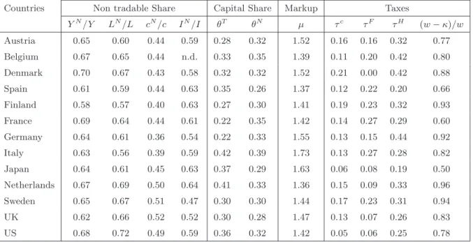
To estimate the sectoral effects of a tax reform, we consider an open economy with a traded and a non traded sector. Our neoclassical framework builds on Turnovsky and Sen [1995] and Coto-Martinez and Dixon [2003]. As Coto-Martinez and Dixon, we let the non traded sector to be imperfectly competitive. Our work differs from analyses by Turnovsky and Sen [1995] and Coto-Martinez and Dixon [2003] in one major respect. They investigate analytically the effects of government spending shocks whereas we provide both an analytical and a quantitative exploration of the effects of tax reforms. One attractive feature of a two-sector model with tradables and non tradables is to cover both the closed-economy and open-economy dimensions of contemporaneous industrialized countries. In particular, empirical evidence documents a sizeable non tradable share in GDP and total employment, averaging to 60% approximately.1

A second key feature of a two-sector model is that a tax reform now produces a change in the relative price of non tradables which triggers a reallocation of resources between the two sectors. Third, our model allows to test if the labor intensive sector always benefits more from the labor tax cut. Fourth, such a model enables us to connect sectoral output responses to the trade balance adjustment.

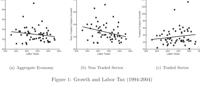
To illustrate the potential importance in evaluating the effects of a tax reform at a sectoral level, we plot in the scatter diagrams of Figure 1 both GDP and sectoral output growth rates in percentage against the labor tax wedge for 27 OECD countries over the period 1994-2004 which has been split into two sub-periods 1994-1998 and 1999-2004.2 _{Figure 1(b) suggests a negative}

1_{Non tradable shares are reported in Appendix A.}

2_{From the early Nineties, European tax systems were requested to achieve conflicting targets: reducing}

unemployment rate and achieving budget balance over the medium run. Hence, the period 1994-2004 is of

10% 20% 30% 40% 50% 60% 0% 2% 4% 6% 8% 10% Labor Taxes Output Growth

(a) Aggregate Economy

10% 20% 30% 40% 50% 60% 0% 2% 4% 6% 8% Labor Taxes

Non Traded Output Growth

(b) Non Traded Sector

10% 20% 30% 40% 50% 60% 0% 2% 4% 6% 8% 10% 12% 14% Labor Taxes

Traded Output Growth

(c) Traded Sector

Figure 1: Growth and Labor Tax (1994-2004)

relationship between labor tax wedge and non traded output.3 By contrast, as illustrated in Figure 1(c), traded output growth and labor tax wedge seem to show an opposite pattern. Furthermore, Figure 1(c) suggests a negative but small relationship between the GDP growth rate and labor taxes across countries. The model’s predictions are in line with these findings: whereas traded and non traded sector vary in opposite direction in the short-run, a cut labor taxes exerts a small impact on GDP (see Figure 1(a)).

Since tax reforms take various forms, we consider three simple and practicable tax restruc-turing: i) two revenue-neutral tax reforms that reduce the marginal tax wedge by shifting the tax burden from labor to consumption taxes and ii) one labor tax reform keeping the marginal tax wedge constant by shifting the tax burden from employers to employees.4 _{We show formally}

that regardless of its type, a tax restructuring crowds-in both consumption and investment, and raises employment. These results confirm earlier conclusions reached by Mendoza and Tesar [1998] who, in particular, experiment a tax reform replacing the labor income tax with a consumption tax within a two-country framework. The intuition behind these results are as follows. The fall in labor cost induces firms to raise wages which in turn stimulate labor supply. The consecutive increase in labor income pushes up consumption. To meet greater demand, the economy must accumulate capital. These conclusions are in line with the VAR

particular interest as a lot of countries compensate for labor tax cut by an increase in the consumption tax rate.

3_{Sample includes 27 countries: Australia, Austria, Belgium, Canada, Czech Republic, Denmark, Finland,}

France, Germany, Greece, Hungary, Iceland, Ireland, Italy, Japan, Mexico, Netherlands, New Zealand, Norway, Poland, Portugal, Slovak Republic, Spain, Sweden, Switzerland, UK, US. The labor tax wedge is taken from OECD, Historical rates. Tax wedge includes income tax paid by workers and social security contributions levied on employees and their employers for a single person at 100% of average earnings, no child. Method of calculation of non traded and traded output is described in Appendix A. Source: KLEMS.

4_{While the two revenue-neutral tax reforms lower the marginal tax wedge, we consider a third strategy}

which involves simultaneously cutting payroll taxes and raising labor income taxes so as to keep the tax wedge constant. Whereas this labor tax restructuring does no longer keep the tax revenue fixed, it allows us to focus on the composition on the tax wedge rather than its level.

evidence documented by Blanchard and Perotti [2002] and Mertens and Ravn [2010], as long as the tax reform is unanticipated. Furthermore, like Mendoza and Tesar, we find that trade in world financial markets allows the open country to finance higher investment without sacri-ficing consumption in the short-run. Hence, the open economy runs short-run current account deficits which are compensated by a trade balance surplus in the long-run.

By differentiating between tradables and non tradables, our model yields new predictions at a sectoral level. Following a tax reform, the non traded sector strongly expands on impact while traded output falls dramatically. The reason is that the open country runs a deficit in the trade balance in the short-run triggered by the investment boom. The fall in net exports requires a drop in traded output which is achieved through a reallocation of resources towards the non traded sector. Henceforth, sectoral outputs move in opposite direction in the short-run, which implies that tax rates produce a small impact on GDP. By contrast, in the long-run, a tax reform stimulates both traded and non traded output. The reason is that the debt accumulated during the transition is serviced by a rise in net exports in the long-run. As consumption increases, such a surplus in the trade balance is achieved through a rise in traded output along the transitional path, triggered by the reallocation of resources towards the traded sector.

As it is currently assumed in the two-sector literature, for analytical simplicity, we first consider that the traded sector is more capital intensive than the non traded sector in discussing the macroeconomic effects of tax reforms.5 _{Considering the case of reversal capital intensities,}

numerical experiments show that the effects are roughly similar. By contrast, we find that sectoral output responses are significantly sensitive to the elasticity of labor supply and the tradable content of consumption expenditure. First, irrespective of sectoral capital intensities, as labor supply gets more responsive, non traded output expands more while traded output falls by a larger amount on impact. Second, we find that a fall in the tradable content of consumption expenditure amplifies the heterogeneity in sectoral output responses, only when the non traded sector is relatively more capital intensive.

We also conduct a sensitivity analysis with respect to the degree of competition in the

product markets, by making the markup endogenous.6 _{The change in the markup provides an}

additional channel through which a tax reform impinges on sectoral outputs. We find that, by lowering the markup on impact, a tax reform stimulates further capital accumulation and yields a larger current account deficit. Hence, non traded output expands more while traded

5_{See e.g. Obstfeld [1989], Mendoza [1995], or Coto-Martinez and Dixon [2003] who assume that the traded}

sector is more capital intensive. Yet, our estimation of sectoral capital income shares in output show that the non traded sector is relatively more capital intensive in five countries over thirteen.

6_{Coto-Martinez and Dixon [2003] consider the case of a fixed markup.}

output falls by a larger amount. The change of the markup amplifies the opposite responses of sectoral outputs, the net overall effect on GDP remaining roughly similar.

The remainder of the paper is organized as follows. Section 2 outlines the specification of a two-sector model with traded and non traded goods. In Section 3, we discuss the short-run and long-short-run effects of three tax reforms which involve cutting labor taxes. Section 4 provides a quantitative exploration of the sectoral effects and conducts a sensitivity analysis with respect to key parameters. In Section 5, we analyze to which extent our results are modified by considering that the non traded sector is more capital intensive. Section 6 explores quantitatively the case of an endogenous markup. Section 7 summarizes our main results and concludes.

2

The Framework

We consider a small open economy that is populated by a constant number of identical house-holds and firms that have perfect foresight and live forever. The country is small in both world goods and capital markets and faces given world interest rate,r?_{. A perfectly competitive}

sec-tor produces a traded good denoted by the superscriptT that can be exported and consumed

domestically. An imperfectly competitive sector produces a non traded good denoted by the superscript N which is devoted to physical capital accumulation and domestic consumption.7

The traded good is chosen as numeraire.89

2.1 Households

At each instant the representative agent consumes traded goods and non traded goods de-noted respectively bycT and cN, which are aggregated by a constant elasticity of substitution function: c¡cT, cN¢= · ϕφ1 ¡cT¢ φ−1 φ _{+ (1−ϕ)}φ1 ¡cN¢ φ−1 φ ¸ φ φ−1 , (1)

withϕthe weight attached to the traded good in the overall consumption bundle (0< ϕ <1) and φthe intratemporal elasticity of substitution (φ >0).

The agent is endowed with a unit of time and supplies a fraction L(t) as labor and the remainder, l≡1−L is consumed as leisure. At any instant of time, households derive utility

7_{As stressed by Turnovsky and Sen [1995], allowing for traded capital investment would not affect the results.}

Furthermore, like Burstein et al. [2004], non tradable investment accounts for a large share of total investment (i.e. 60%).

8_{The price of the traded good is determined on the world good market and exogenously given for the small}

open economy.

9_{More details on the model as well as the derivations of the results which are stated below are provided in}

an Appendix which is available on request.

from their consumption and leisure. Households decide on consumption and worked hours by maximizing lifetime utility:

U = Z _∞ 0 ( 1 1− 1 σc c(t)1−σc1 −γ 1 1 + 1 σL L(t)1+σL1 ) e−βtdt, (2)

where β is the consumer’s discount rate,σc>0 is the intertemporal elasticity of substitution

for consumption,σL>0 is the Frisch elasticity of labor supply;

Factor income is derived from supplying laborLat a wage ratewand capitalK at a rental raterK.10 Labor is taxed at rateτH. The wage tax is levied on households’ wage income above a certain thresholdκ, which represents the personal tax allowance. Thus,wA_{=w−(w−κ)τ}H

corresponds to the after-tax wage. As long as tax allowances are positive, the tax system is progressive which means that the average tax burden rises with the wage rate. In addition, households accumulate internationally traded bonds,b(t), that yields net interest rate earnings

r?_{b(t). Denoting by Z lump-sum transfers from the government, the households’ flow budget}

constraint writes as follows: ˙

b(t) =r?b(t) +rK(t)K(t) +wA(t)L(t) +Z−pc(p(t)) (1 +τc)c(t)−p(t)I(t), (3)

wherepc is the consumption price index which is a function of the relative price of non traded

goods p. The last two terms represent households’ expenditure which include purchases in

consumption goods inclusive of consumption tax rateτc_{, and investment expenditure pI.}

Ag-gregate investment gives rise to overall capital accumulation according to the following dynamic equation:

˙

K(t) =I(t)−δ_KK(t). (4)

where we assume that physical capital depreciates at rate δ_K. From now thereon, the time-argument is suppressed for clarity purpose.

Denoting byλthe co-state variable associated with equation (3), the first-order conditions characterizing the representative household’s optimal plans are:

c= (pc(1 +τc)λ)σc, (5a) L= µ _¯ λ γL wA ¶_σL , (5b) ˙ λ=λ(β−r?), (5c) rK p −δK+ ˙ p p =r ?_{, (5d)}

and the appropriate transversality condition. To generate an interior solution for the marginal utility of wealth λ, we require the time preference rate to be equal to the world interest rate.

10_{We abstract from capital income tax which is beyond the scope of this paper.}

This standard assumption made in the literature implies that the marginal utility of wealth,

λ, must remain constant over time, i. e. λ= ¯λ. 2.2 Firms

There are two sectors of production in the model producing a traded goodT and a non traded good N. The traded and non traded sectors face two cost components: a capital rental cost equal to rK_{, and a labor cost equal to w}F _{= w}¡_{1 +τ}F¢ _{with τ}F _{the the employer’s part of}

labor taxes.

The traded sector is assumed to be perfectly competitive and use capitalKT _{and laborL}T

according to a constant returns to scale production function,YT _=F¡_KT_{, L}T¢_{, which has the}

usual neoclassical properties of positive and diminishing marginal products. The first order conditions derived from profit-maximization in the traded sector state that factors are paid to their respective marginal products.

The final non traded output,YN, is produced in a competitive retail sector using a constant-returns-to-scale production which aggregates a continuum measure one of sectoral non traded goods.11 We denote byω > 0 the elasticity of substitution between any two different sectoral goods. In each sector, there areN >1 firms producing differentiated goods that are aggregated into a sectoral non traded good. We denote by² >0 the elasticity of substitution between any two varieties. We assume that the elasticity of substitution between any two goods within a sector is higher than the elasticity of substitution across sectors, i.e. ² > ω (see e.g. Jaimovich and Floetotto [2008]). Within each sector, there is monopolistic competition; each firm that produces one variety is a price setter. Output Xi,j of firm i in sector j is produced using

capital and labor, i.e. Xi,j =H(Ki,j,Li,j). Each firm chooses capital and labor by equalizing

markup-adjusted marginal products to the marginal cost of inputs, i. e. H_K/µ = rK_{, and} HL/µ=wF, whereµis the markup over marginal costs. Aggregate non traded output is equal

to YN _{= NX =H}¡_KN_{, L}N¢_{. We assume that there is a large number of firms within each}

sector so that each single intermediate producer is small relative to the economy and thereby each producer in one sector faces a constant price elasticity of demand². Hence, one producer of a variety charges a constant markup denoted byµ= _e−e₁ withethe price-elasticity of demand equal to ² as the number of competitors is large. In section 6, we relax this assumption and rather assume that a finite number of firms operate within each sectors producing non tradable varieties.12 _{We further assume instantaneous entry which implies that the zero profit condition}

11_{The setup builds on Jaimovich and Floetotto [2008] and thereby details of derivation are relegated to the}

Appendix available on request.

12_{As stressed by Yang and Heijdra [1993], departing from the usual assumption made by Dixit and Stiglitz}

[1977] implies that the price elasticity of demand becomes an increasing function of the number of firms and

holds at each instant of time.

Denoting by ki _{≡ K}i_/Li _{the capital-labor ratio for sector i = T, N, we express the}

production functions in intensive form, that is f¡kT¢ ≡ F¡KT, LT¢/LT and h¡kN¢ ≡ H¡KN_{, L}N¢_/LN_{. Production functions are supposed to take a Cobb-Douglas form: f}¡_kT¢₌

¡

kT¢θT,andh¡kN¢=¡kN¢θN,whereθT and θN represent the capital income share in output in the traded and non traded sector, respectively. Since inputs can freely move between the two sectors, marginal products in the traded and the non traded sector equalize:

θT ¡kT¢θT−1= p µθ N¡_kN¢θN−1_≡rK_{, (6a)} ¡ 1−θT¢ ¡kT¢θT = p µ ¡ 1−θN¢ ¡kN¢θN ≡wF. (6b)

Static efficiency conditions (6a)-(6b) state that sectoral marginal revenue products must equal-ize to the labor producer cost wF and capital rental rate rK. System (6a)-(6b) can be solved for sector capital intensities ratios: kT _=kT _{(p) and k}N _=kN_(p).

Aggregating labor and capital over the two sectors, we obtain the resource constraints for both inputs:

LT +LN =L, KT +KN =K. (7)

2.3 Government

The final agent in the economy is the government who finances lump-sum transfers to house-holds Z together with public spending falling on the tradedgT _{and the non traded good pg}N

by raising taxes on consumption, τcpcc, and labor,

£

τH(w−κ) +τFw¤L, according to the following balanced condition:

τcpcc+

£

τH(w−κ) +τFw¤L=Z+gT +pgN. (8)

2.4 Macroeconomic Dynamics

The adjustment of the open economy towards the steady-state is described by a dynamic system which comprises the dynamic equation for the relative price of non traded goods (5d) which equalizes the return on domestic capital and traded bonds r?_{. The second equation is}

the accumulation equation for physical capital which clears the non traded good market along the transitional path. Solving first-order conditions for output and consumption, the market clearing condition for the non traded good writes as:

˙

K =YN(K, L, p)/µ−cN¡¯λ, p, τc¢−gN −δKK, (9)

that the markup turns out to be endogenous.

where L =L¡¯λ, p, τF, τH, µ¢ is the short-run static solution of eq. (5b); consumption in the non traded good cN _{is equal to α}

cpcc/pwith αc is the non tradable content in consumption

expenditure. Solving eq. (5a) for consumption, the short-run static solution forcN follows. It is worthwhile to notice that a labor tax cut, i.e. a fall inτF _orτH_{, affects the macroeconomic}

equilibrium by modifying labor supply decisions.

Dynamic equations (5d)-(9) form a separate subsystem in p and K.13 _{Denoting by a tilde}

the steady-state value, stable solutions forK and pwrite as:

K(t)−K˜ = ³ K0−K˜ ´ eν1t_{, p(t)−p˜=ω}1 2 ³ K(t)−K˜ ´ , (10) where ω1

2 ≤ 0 is the eigenvector associated with stable eigenvalue ν1. If kT > kN, we have

ω₂1 = 0, so that the relative p, consumption, labor, and thereby savings adjust immediately to their steady-state levels. By contrast, with the reversal of capital intensities, transitional dynamics for the consumption-side variables are restored as ω₂1 <0. Substituting (9) and (8) into (3), we obtain the dynamic equation for the current account denoted byca:

˙

b=r?b+YT (K, L, p)−cT ¡λ, p, τ¯ c¢−gT, (11)

wherecT _{= (1−α}

c)pcc is consumption in the traded good with (1−αc) the tradable content

in consumption expenditure. Equation (11) states that the current account is equal to the trade balance denoted by nx, i.e. nx ≡ YT _−cT _−gT_{, plus interest receipts on outstanding}

assets.

2.5 Steady-State

We now discuss the salient features of the steady-state. Setting ˙p = 0 into eq. (5d),

we obtain the equality between the after-tax rate of return on domestic capital income

θN

³

˜

kN

´_θN₋₁

/µ−δK and the exogenous world interest rate, r?, that determines the

steady-state value of the relative price of non tradables ˜p. The long-run level of premains unaffected by a tax restructuring, as long as the markup is fixed. The steady-state level ofp determines the wage rate ˜w= θT[kT(˜p)]

θT−1

1+τF . By substituting the wage rate into the labor supply decision

evaluated at the steady-state, we get ˜L=

n ¯ λ γL £ ˜

w−( ˜w−κ)τH¤oσL_{. For given ¯λ, a cut in τ}F

raises the wage rate and thereby stimulates labor supply.

Setting ˙K= 0 into eq. (9) yields the market-clearing condition for the non traded good: 1

µY

N³_K,˜ _L,˜ _p˜´_=cN¡_λ,¯ _{p, τ˜} c¢_{+ ˜I+g}N_{, (12)}

13_{Since the number of predetermined variables (K) equals the number of negative eigenvalues (denoted byν1)}

and the number of jump variables (p) equals the number of positive eigenvalues (denoted byν2), the equilibrium yields a unique one-dimensional stable saddle-path, irrespective of the relative sizes of sectoral capital-labor ratios.

where ˜I =δKK˜.

Setting ˙b= 0 into eq. (11) yields the market-clearing condition for the traded good:

YT ³ ˜ K,L,˜ p˜ ´ =−r?˜b+cT¡¯λ,p, τ˜ c¢+gT. (13)

The intertemporal solvency condition can be solved for the shadow value of wealth:

³

˜_b−b0´_{= Ω}³_K˜ _−K0´_{, (14)}

where Ω<0 describes the effect of capital accumulation on the the external asset position and

K0 andb0 are the initial stocks of capital and foreign assets.14

Eqs. (12)-(14) jointly determine the steady-state values of physical capital, ˜K, foreign bonds holding, ˜b, and the shadow value of wealth, ¯λ. It is worthwhile to note that eq. (14) connects eqs. (12) and (13), and thereby sectoral outputs. More precisely, an investment boom

˜

I stimulates non traded output ˜YN _{and traded output ˜Y}T _{too since capital accumulation yields}

a drop in ˜b. The reason is that the fall in interest receipts due to lower traded bonds holding must be exactly matched by a long-run improvement in the balance of trade which exerts a positive impact on ˜YT.

3

Effects of Tax Reforms: An Analytical Exploration

Since tax reforms can take various forms, we consider three types of tax restructuring. We explore two revenue-neutral tax reforms which involve simultaneously either cutting payroll taxes by dτF < 0 or labor income taxes by dτH < 0 and raising the consumption tax by dτc _{> 0. While these tax reforms cause a fall in the tax wedge, we consider a third tax}

restructuring which involves simultaneously cutting payroll taxes by dτF <0 and raising the wage income tax rate dτH _{>0 that leaves unchanged the tax wedge. The third policy allows us}

to analyze a shift in the composition of the labor taxation rather than a change in the marginal tax wedge defined as the difference between the producer wage and the after-tax marginal wage expressed as a percentage of the producer cost: τM _{= 1−}(1−τH)

(1+τF₎ (see e.g. Heijdra and Ligthart

[2009]). Moreover, For pedagogical purpose, we assume that the traded sector is more capital intensive than the non traded sector, i.e. kT _{> k}N_{, as it is commonly assumed in the two-sector}

literature. We explore the case of reversal capital intensities in section 5.

14_IfkT _{> k}N_{, then Ω =−p <˜ 0. Ifk}N _{> k}T_{, Ω =−p˜}h_{1 +} ω₂1 ˜ pν2 ³ σcc˜N−σLL˜k˜T(ν2+δK) ˜Λ ´i with 0<Λ≡ (1−τH₎ h (1−τH₎+τ H κ w i _<1.

3.1 Revenue-Neutral Tax Reforms

We analyze first the long-run effects of a revenue-neutral tax reform. To avoid confusion, we denote by¯¯j,c the effects of a fall in the labor tax by dτj _{<0 (j=F, H) coordinated with a rise}

in the consumption tax rate by dτc¯¯j,c which is endogenously determined so as the government budget constraint is met. Assuming that the stock of financial wealth is positive, the labor tax base is smaller than the consumption tax base.15 Hence, τc must increase less than the drop in labor tax.16

The long-term change of x = c, L, K, nx following a shift from labor tax to consumption tax is equal to the sum of the expansionary impact of the labor tax cut by dτj _{<0 (j =F, H)}

financed by lump-sum taxes (i.e. ∂x˜

∂τjdτj >0) and the recessionary effect triggered by the rise

in the consumption tax rate by dτc¯¯j,c _(i.e. ∂˜x ∂τcdτc ¯ ¯j,c _<0):17 d˜x¯¯j,c = ∂x˜ ∂τjdτj+ ∂x˜ ∂τcdτc ¯ ¯j,c ≡Φj,c ∂x˜ ∂τjdτj >0, j=F, H, (15)

where 0<Φj,c _{<1 (j =F, H). The second equality of eq. (15) states that the long-run change}

in x = c, L, K, nx following a tax reform is simply a scaled-down version of the long-term

changes ofxafter a lump-sum tax financing labor tax cut. Consequently, a tax reform shifting the labor tax to the consumption tax stimulates employment and consumption, and raises both the capital stock and net exports. The reason is that a labor tax cut induces agents to supply more labor. The consecutive increase in the after-tax labor income boosts consumption. In the same time, the labor inflow in the non traded sector raises output in that sector which in turn stimulates capital accumulation. The capital inflow in the traded sector raises its output which results in a long-run improvement in the balance of trade. A tax reform produces the same effects but now their size are moderated due to the scaling-down term 0<Φj,c_<1.

Moreover, a tax reform stimulates further c, L, K, nx as the scaled-down term Φj,c gets closer to unity. If the labor tax cut was financed by a rise in lump-sum taxes, Φj,c _would

be equal to unity, and the higher bound of the net overall outcome of a tax reform would be obtained. In contrast, if the stock of financial wealth was equal to zero, the consumption tax

15_{At the steady-state, denoting by a ≡b+pK the stock of financial wealth, we have: r}?_{a˜+Z+ ˜w}A_{L˜ =} pc(1 +τc) ˜c. As long asr?˜a+Z >0, the consumption tax base is larger than the labor tax base.

16_{Both the labor tax cut and the rise inτ}c _{yields opposite effects on tax receipts. On the one hand, a labor}

tax cut lowers public revenue, keeping unchanged consumption and employment. Second, a labor tax rate cut raises employment and consumption, and thereby tax revenues. While analytically, the net overall effect cannot be signed, we find numerically that the former effect always more than offsets the latter effect. The same logic applies to a change in the consumption tax rate. We find numerically that the net overall effect on tax revenues of a labor tax cut is close to that following a rise in the consumption tax, in absolute terms. Hence, only the ratio of the labor tax base to the consumption tax base matters in determining the size of the increase inτc_.

17_{Formal details can be retrieved in the Appendix.}

base would be equal to the labor tax base, and a tax reform would produce no effect.18 This situation corresponds to the lower bound of the net overall outcome of a tax reform. The effects of a tax restructuring falls between these two bounds.19

Let now discuss the impact effects. In the casekT _{> k}N_{, the dynamics of the relative price}

degenerate so that labor and real consumption increase immediately to their final long-term levels. Investment is the result of demand and supply reactions in the non traded good market. The increase in total employment induces a labor inflow in the non traded sector which boosts

YN_{. While the initial rise in c}N _{withdraws resources from capital accumulation, the stimulus}

of non traded output is large enough to cause an investment boom on impact. Formally, using stable solution (10), we have: dI(0)¯¯j,c=−ν1d ˜K

¯

¯j,c_{>0. Finally, the open country runs a trade}

balance deficit in the short run given by dnx(0)¯¯j,c =ν₁p˜d ˜K¯¯j,c <0, reflecting the immediate boom in investment as savings remain unchanged.

So far, we have analyzed the effects of a labor tax cut coordinated with a rise in the consumption tax rate, without differentiating between a cut in the employer’s (i.e. τF_{) or}

employee’s (i.e. τH_{) part of labor taxes. A drop in τ}H _{leaves unaffected w and raises the}

after-tax labor income by ( ˜w−κ). A cut inτF _{raises the wage rate and thereby the after-tax}

labor income by ˜w1−τH

1+τF = ˜w

¡

1−τM¢_{, with τ}M _{the marginal tax wedge. Whereas the size of}

the effects after a fall in τH _{decreases with tax progressiveness, the magnitude of the effects}

following a fall in τF _{rises with the marginal tax wedge.}

3.2 A Labor Tax Restructuring

As it is common in the literature investigating the macroeconomic effects of a tax reform, so far we have analyzed revenue-neutral tax reforms. Let now consider that the policy maker wishes to alter the composition of the marginal tax wedge without however, changing its level. We denote by the superscript {F, H}the effects of a tax reform which involves simultaneously cutting the employer’s part of labor tax and increasing the personal income tax dτH _{>0 so as}

to leave unchanged the marginal tax wedge (i. e. dτM _{= 0). A labor tax restructuring requires}

a rise in the personal income tax by an amount given by: dτH¯¯F,H ≡ −1−τH

1 +τFdτ

F ₌¡_τM ₋₁¢_dτF _{>0. (16)}

According to (16), the personal income tax must be increased by a smaller amount than the fall in τF _{for keeping unchanged the marginal tax wedge. Intuitively, since the tax rate on a}

18_{More rigorously, the labor tax base is equal to the consumption tax base ifr}?_{a˜+Z= 0.}

19_{The larger the share of financial wealth in real disposable income, the greater the consumption tax base}

compared to the labor tax base, and thereby the closer to one the scaling-down term Φj,c_{. Hence, the less τ}c

needs to increase for a given labor tax cut to balance the budget and the larger the effects of a tax reform on

c, L, K, nx.

relatively large base is reduced and the tax rate on a relatively small base is increased, the latter must rise by a smaller proportion than the former decreases so as to leave unchanged

τM.

The steady-state change of x=c, L, K, nxfollowing a cut in τF_{, coordinated with a rise in} τH by an amount given by (16), reads:

d˜x¯¯F,H = ΦF,H ∂x˜ ∂τFdτ F ₌ κ ˜ wdτ F_{, (17)}

where 0<ΦF,H _{≡κ/w <˜ 1. Settingκ to zero implies that such a tax reform will produce no}

effects on the economy. Rather, as long as the labor tax scheme is progressive, i. e. κ >0, the labor tax reform leaving constant the tax wedge raises permanentlyx. As for revenue-neutral tax reforms, the steady-state changes inc, L, K, nxare a scaled-down version of their long-term changes following a labor tax cut financed by lump-sum taxes. The scaled-down term is equal toκ/w˜ and thereby depends on the degree of progressiveness of the tax scheme. The stronger the progressiveness in the tax scheme, the larger the increase in the after-tax wage rate and thereby the greater the beneficial effects on employment and overall economic activity. We dot not discuss further the impact effects which are similar to that described for revenue-neutral strategies.

3.3 Output Response

We now investigate in details the response of output at an overall level and importantly at a sectoral level. We denote by ¯¯j,k the effects of a fall in the labor tax by dτj _{< 0 (j = F, H)}

financed by a rise inτk _{(k=c, H).}

3.3.1 GDP Response

We analyze first the response of GDP to highlight the role of trade balance. Using the fact that in the long-run, overall output equalizes its demand counterpart, and differentiating, the long-run GDP response is given by:20

d ˜Y¯¯j,k =pcd˜c

¯

¯j,k_{+ d ˜nx}¯_¯j,k_{+ ˜pd ˜I}¯_¯j,k _{>0, (18)}

where d˜x¯¯j,k >0 (with ˜x= ˜c,I,˜ nx˜) is given by (15) or (17) depending on the type of the tax reform. According to (18), the domestic demand boom for both consumption and investment goods stimulates GDP. Furthermore, the improvement in the balance of trade to service the

20_{Using the market-clearing condition, i. e.} Y˜N

µ = ˜c

N _+gN _{+ ˜I, and the current account, i. e. Y˜}T ₌

¡ ˜

cT_+gT¢_−r?_{˜b, aggregating and differentiating, we get (18), keeping in mind that the steady-state level of the}

relative price of non tradables remains unchanged.

debt accumulated during the transition raises further ˜Y. In a closed economy framework, the latter demand component vanishes. Hence, as stressed by Mendoza and Tesar [1998], a closed economy model would underestimate the beneficial effects of a tax restructuring since the trade balance surplus magnifies the effects of a tax reform on GDP in the long-run.

Linearizing aggregate demand for the domestic good, i. e. Y = pc(p(t))c(t) +

¡

gT _+p(t)gN¢_{+p(t)I(t) +nx(t), evaluating at time t = 0 and differentiating enables us to}

decompose the GDP response in its demand counterparts as follows:21

dY(0)¯¯j,k =pcdc(0)

¯

¯j,k_{+ ˜pdI(0)}¯_¯j,k_{+ ˜Y}N_dp(0)¯_¯j,k_{+ dnx(0)}¯_¯j,k_{>0, (19)}

where dp(0)¯¯j,k = 0 as long as kT _{> k}N _{since the dynamics for the relative price degenerate}

in this case. According to (19), the initial response of GDP is driven by the initial demand boom for both consumption and investment goods. Yet, as reflected by the last term, the trade balance deficit lowers the size of the GDP increase. As long askT _{> k}N_{, savings remain}

unchanged. Hence, the worsening in the external asset position mirrors exactly the investment boom. Consequently, the initial response of GDP is only driven by higher consumption. Since consumption adjusts immediately to its long-run level, the short-run increase in GDP is smaller than that in the long-run.22

3.3.2 Sectoral Output Responses

We now analyze if the traded and non traded sectors are affected uniformly by a tax reform. Using the market-clearing condition together with the zero current account equation, we can derive the steady-state changes of non traded and traded output, respectively:

1

µd ˜Y

N¯_¯j,k _{= d˜c}N¯_¯j,k_{+ d ˜I}¯_¯j,k _{>0, (20a)}

d ˜YT¯¯j,k = d ˜nx¯¯j,k+ d˜cT¯¯j,k >0. (20b)

Since a tax restructuring raises after-tax labor income and induces households to consume more, demands for both traded and non traded consumption goods expand. Additionally, higher investment in physical capital and net exports raise further non traded and traded output, respectively. Interestingly, in the long-run, sectoral outputs are positively correlated. More precisely, the larger the economic boom in the non traded sector, the more traded output increases in the long-run. The explanation is that the greater the investment boom is, the larger the accumulated debt and the more net exports must increase.

21_{An alternative way to determine the initial response of GDP is to use the fact that Y ≡ Y}T ₊ p

µY

N_.

Keeping in mind that the capital stock is initially predetermined and differentiating, we obtain dY(0)¯¯j,k =

wF_dL(0)¯_¯j,k

>0. Since worked hours increase on impact, GDP rises in the short-run.

22_{In the casek}N_{> k}T_{, we reach similar conclusions since savings play little role as we consider time separable}

preferences and we assume that the tax reform is permanent.

We now evaluate if the sectoral outputs move in opposite direction. The sectoral output responses in the short-run are:

1

µdY

N₍₀₎¯_¯j,k _{= dc}N₍₀₎¯_¯j,k_{+ dI(0)}¯_¯j,k _{>0, (21a)}

dYT(0)¯¯j,k = dnx(0)¯¯j,k+ dcT(0)¯¯j,k≷0. (21b)

According to (21a), the demand boom for non tradables causes an expansion in the non traded sector. With regard to the traded sector, the dramatic drop in net exports on impact now counteracts the positive influence of higher consumption. If kT _{> k}N_{, it can be proven}

ana-lytically that traded output falls on impact. The intuitive explanation is that households get richer due to a higher after-tax wage and greater labor supply. Hence, they are induced to consume further. They raisecN _{and c}T_{. But since the traded sector is more capital intensive,}

it experiences a labor outflow on impact so that traded output declines. Hence, the rise incT

reflects additional imports which results in a trade balance deficit.23

4

Tax Reforms: A Quantitative Exploration

In this section, we analyze the effects of tax reforms quantitatively. For this purpose we solve the model numerically. In the following, we thus first discuss parameter values before turning to the long-term and short-term effects of the tax substitutions.

4.1 Benchmark Parametrization

We start by describing the calibration of consumption-side parameters that we use as a baseline. The world interest rate, which is constrained to equalize the subjective time discount rate β, is chosen to be 3%. The intertemporal elasticity of substitution σ_c is set to 0.7 and the intratemporal elasticity of substitution φ to 2 (see e.g. Cashin and Mc Dermott [2003]). One critical parameter is the intertemporal elasticity of substitution for labor supply σ_L. In our baseline parametrization, we setσL= 0.5, in line with evidence reported by Domeij and Flod´en

[2006]. An additional critical parameter isϕ which is set to 0.5 in the baseline calibration to target a tradable content in total consumption expenditure (i.e., 1−αc) of 50%. Below, we

conduct a sensitivity analysis with respect to these two parameters, i.e. we setσ_L to 0.2 and 1, andϕto 0.1 and 0.9.24 _{For reason of space, we focus on the shift of employers’ labor taxes}

(i.e. a fall in τF_{) towards consumption tax (i.e. a rise in τ}c_{) in evaluating the sensitivity of}

numerical results toσL and ϕ.

23_{More precisely, physical capital accumulation requires a shift of resources towards the non traded sector.}

Hence, traded output falls. Because consumption in traded good rises, additional demand yields higher imports.

24_{Raisingϕfrom 0.1 to 0.9 increases the tradable share in GDPY}T_{/Y from 24% to 62%.}

We now describe the calibration of production-side parameters. We let physical capital to depreciate at a rateδK = 4% to generate an investment-GDP ratio of 20% which is consistent

with data from developed countries. Sectoral capital income shares in output take two different values depending on whether the traded sector is more or less capital intensive than the non traded sector. In line with our estimates, whenkT > kN, the values ofθT andθN are set to 0.4 and 0.3 respectively. Alternatively, in the case kN _{> k}T_{, we choose θ}T _{= 0.3 and θ}N _{= 0.4.}25

The elasticity of substitution between varieties of non traded goods, ² is set to 3 to target a markup of 1.5, in line with our estimates (see Appendix A). In the case of an endogenous markup explored in section 6, keeping²unchanged, we set the elasticity os substitution between sectoral goods ω to 2 to target a markup of 1.5.

To set τc_{, τ}F _{and τ}H_{, we estimated effective tax rates for thirteen OECD countries over}

2000-2007. The consumption taxτc_{is set to 13%, the employer’s part of labor taxesτ}F _{to 16%}

and the wage income tax τH _{to 31%. In evaluating quantitatively the effects of a tax reform,}

we consider a labor tax cut by 5 percentage points. Tax allowances κ is set to 0.3 to obtain a share of taxable income into the gross wage earnings (w−κ)/w of 0.7. We set gN _{and g}T

to target a non tradable share of government spending of 90% and government spending as a share of GDP of 20%.

4.2 Long-Run Effects: A Quantitative Sectoral Decomposition We now provide a quantitative exploration of the size of long-run effects. 4.2.1 Macroeconomic Effects

Using simple algebra, we have shown previously that long-term changes of consumption, em-ployment and capital stock following a tax restructuring are a scaled-down version of the steady-state changes following a lump-sum tax financing labor tax cut. For the baseline parametrization, we find that the scaling-down term displays the same magnitude across the types of tax reforms. More precisely, for our benchmark parametrization, Φj,k _{is equal to 0.25,}

approximately. Hence, the size of the long-run effects are similar across the three tax reforms.26

As discussed in section 3, a tax restructuring stimulates both consumption and investment, and improves the balance of trade. To disentangle the contribution to each GDP component

25_θT _{= 0.4 andθ}N_{= 0.3 correspond approximately to average for countries with k}T _{> k}N _{(see Table 3). In}

the case of reversal capital intensities, we consider symmetric values for θN _{and θ}T _{so that the gap between}

sectoral capital intensities remain unchanged.

26_{For our baseline calibration, as the tax wedge is high and the tax scheme displays weak progressiveness}

of tax progressiveness, a tax reform which involves cutting the wage income tax paid by households τH _while

raising the consumption tax rate produces the larger effects onc, L, K.

to the rise in overall output, we scaled steady-state changes of consumption, investment and the balance of trade by initial GDP. Numerical results are summarized in Table 1B. We find that two-third of the GDP growth is driven by the rise in consumption. The remaining share is attributed to the steady-state improvement in the balance of trade and the investment boom.

4.2.2 GDP Response

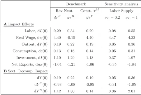
Table 1D summarizes the numerical values for both overall and sectoral output responses. For the benchmark parametrization, the steady-state response of GDP falls in the range between 0.26-0.30, depending on the tax reform which is implemented. More importantly, as emphasized previously, sectoral outputs are positively correlated in the long-run. Interestingly, we find that that tradable output expands more than non tradable output: ˜YT _{rises by 0.15% of GDP while}

˜

YN _{increases by 0.11%. The sizeable expansion in the traded sector relies upon the long-run}

improvement in the balance of trade. While the tradable share in overall output is about 40%, its contribution to GDP increase is close to 60%.

4.3 Impact Effects: A Quantitative Sectoral Decomposition

The sectoral decomposition of the effects of a tax restructuring allows to highlight the prop-agation mechanism. The impact responses of sectoral outputs are summarized in the second and third line of Table 1E. Interestingly, sectoral outputs vary in opposite direction in the short-run. More precisely, the increase in non traded output is four times larger than that of GDP and falls between 0.67% and 0.79% of initial GDP approximately, depending on the tax restructuring which is implemented. By contrast, the traded sector experiences a severe decline in its output which falls between 0.5% and 0.59% of initial GDP approximately. The reason for opposite responses in sectoral output stems from the shift of resources across sectors. The initial stimulus of hours worked shifts resources from the traded towards the non traded sector which is labor intensive. In the same time, households consume more due to higher after-tax labor income. While tradable output decreases, about half of the additional income is devoted to imports which causes a current account deficit. In section 5.1, we find that sectoral outputs also vary in opposite direction in the case of reversal capital intensities, i.e. kN _{> k}T_.

4.4 Dynamics Effects

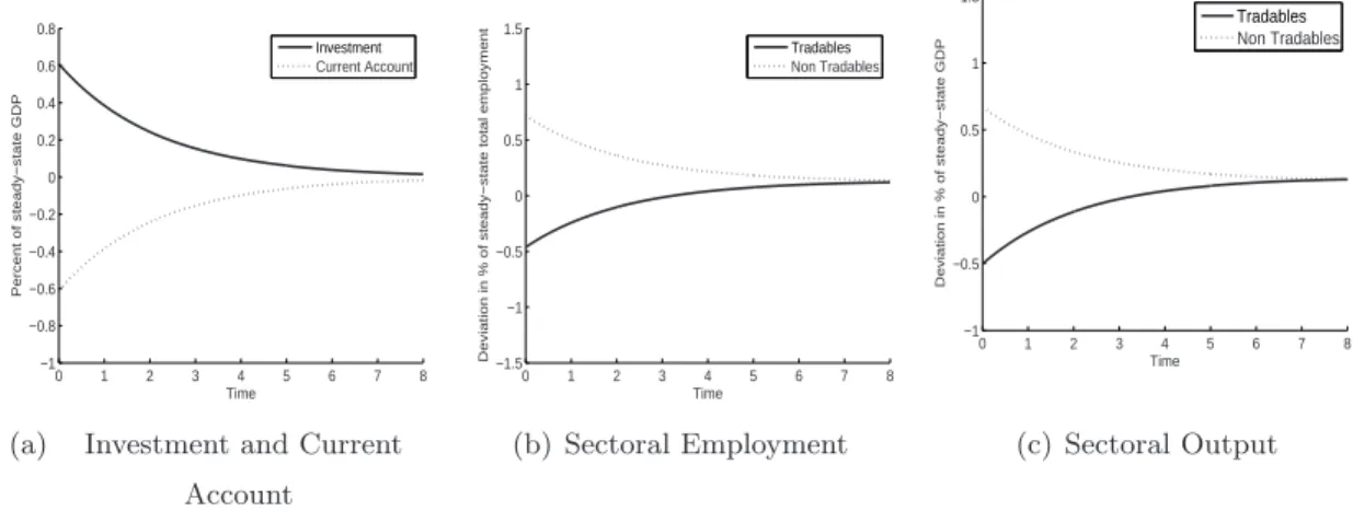
We now investigate the dynamic effects. Computed transitional paths of key variables are displayed in Figures 2 where we consider a shift of the tax burden from labor taxes (i. e. a cut inτF_{) to consumption taxes (i. e. a rise inτ}c_{). Investment and the current account are scaled}

by initial GDP while sectoral outputs are expressed as deviations from initial steady-state

values scaled by initial GDP (in percentage). Reactions of sectoral employment are scaled by initial total employment.

As illustrated in Figures 2(b)-2(c), employment increases by about 0.7% in the non traded sector which boostsYN _{by 0.67%. Conversely, the traded sector experiences a labor outflow by}

almost -0.5% which drives down its output by 0.5%. As shown in Figure 2(a), the labor inflow in the non traded sector triggers an investment boom which drives the current account into deficit in the short-run by -0.5% of GDP. As the economy accumulates physical capital over the transition, the traded sector which is more capital intensive expands. As displayed in Figures 2(b)-2(c), the investment boom shifts resources towards the traded sector so that employment and thereby output rises in that sector. After 3 years, traded output exceeds its initial level and converges towards a new higher steady-state level. While the initial boom in the non traded sector slows down, the rate of growth remains positive over the entire adjustment.

4.5 Sensitivity Analysis

As expected, the size of labor supply responsiveness exerts a sizeable effect on steady-state GDP

response and GDP components. As σL is raised from 0.2 and 1, the GDP response increases

from 0.08% to 0.48% approximately. By contrast, raising the tradable share of consumption by increasing ϕdoes not modify significantly the long-run GDP response. The reason is that the relative price remains unchanged in the long-run.

Interestingly, labor supply also affects significantly the contribution of traded output to the long-run GDP expansion. While settingσL to 0.2 implies that half of the GDP growth can be

attributed to the traded sector, its contribution is close to 60% if σL is set to 1. The reason

is that, as labor supply gets more responsive, the traded sector experiences a greater labor outflow on impact which triggers a larger current account deficit. Hence, net exports must increase more in the long-run which boosts further ˜YT_.

Additionally, increasing the tradable good content (i.e. raisingϕ) plays a significant role in driving the size of the long-term responses of sectoral outputs. Settingϕ= 0.9 implies that the growth in traded output contributes to 80% of GDP increase. The reason is that consumption in the traded good expands by a larger amount which magnifies the increase in ˜YT_{. Since}

GDP growth is unaffected by the value of ϕ, a rise in the traded good content shifts resources towards the traded good sector.

Finally, raising σ_L amplifies considerably the heterogeneity in sectoral output responses in the short-run. Increasing σL from 0.2 to 1, the decline in YT becomes more pronounced

(-0.90% against -0.16%) and the rise in YN _{gets larger (1.20% against 0.21%). Because the}

relative price remains unchanged, raising ϕ does not modify significantly the magnitude of

0 1 2 3 4 5 6 7 8 −1 −0.8 −0.6 −0.4 −0.2 0 0.2 0.4 0.6 0.8 Time Percent of steady−state GDP Investment Current Account

(a) Investment and Current Account 0 1 2 3 4 5 6 7 8 −1.5 −1 −0.5 0 0.5 1 1.5 Time

Deviation in % of steady−state total employment

Tradables Non Tradables (b) Sectoral Employment 0 1 2 3 4 5 6 7 8 −1 −0.5 0 0.5 1 1.5 Time Deviation in % of steady−state GDP Tradables Non Tradables (c) Sectoral Output

Figure 2: Transitional Paths after a Labor-Consumption Tax Restructuring (Fixed Markup)

sectoral output responses.

5

A more Capital Intensive Non Traded Sector

So far, we have assumed that the traded sector was more capital intensive than the non traded sector, as it is commonly assumed in the two-sector theoretical literature for analytical con-venience. Yet, our estimation of sectoral shares of capital income in output show that half of industrialized countries displays a non traded sector which is more capital intensive. Given its empirical relevance and for robustness purpose, we analyze to which extent our results are modified by considering that the non traded sector is more capital intensive. Such an analysis allows us to test if the non traded sector still benefits the labor tax cut in the short-run, even if it is more capital intensive. Furthermore, we evaluate the sensitivity of our numerical results to the tradable share in consumption expenditure and labor supply responsiveness.

5.1 The Role of Sectoral Capital Intensities

Assuming thatkN _{> k}T _{implies that the dynamics forpdo no longer degenerate. Rather, the}

relative pricepmust rise on impact as the result of higher demand for non tradables and decline along the transitional path to equalize the returns on domestic and foreign assets. Since the temporal path of the relative price is no longer flat, transitional dynamics for consumption and labor are restored. Importantly, the non traded sector experiences a labor outflow which shifts towards the more labor intensive sector. Because the relative price of non tradables strongly appreciates on impact, the consecutive shift of resources triggers an investment boom. With regard to the long-term GDP response, Table 1D shows that the results are weakly sensitive to sectoral capital intensities.

T able 1: Quan titativ e Effects of T ax Reforms (Exogenous Markup) k T > k N k N > k T Benc hmark Sensitivit y analysis Benc hmark Sensitivit y analysis Rev-Neut Const. τ M Lab or Supply T rad. Share Rev-Neut Const. τ M Lab or Supply T rad. Share dτ F dτ H dτ F σL = 0 . 2 σL = 1 ϕ = 0 . 1 ϕ = 0 . 9 dτ F dτ H dτ F σL = 0 . 2 σL = 1 ϕ = 0 . 1 ϕ = 0 . 9 A .T ax Rate changes d ˜ τ c +3.4 +4.0 +3.9 +3.1 +3.4 +3.4 +3.2 +3.7 +3.6 +3.0 +3.2 +3.3 d ˜ τ F -5.0 -5.0 -5.0 -5.0 -5.0 -5.0 -5.0 -5.0 -5.0 -5.0 -5.0 -5.0 d ˜ τ H -5.0 +3.0 -5.0 +3.0 B .Steady-State Effects Lab or, d ˜L 0.26 0.30 0.26 0.08 0.46 0.27 0.25 0.29 0.33 0.29 0.12 0.48 0.30 0.29 Real W age, d ˜ w 4.52 0.00 4.52 4.52 4.52 4.52 4.52 4.52 0.00 4.52 4.52 4.42 4.52 4.52 Output, d ˜Y 0.26 0.30 0.27 0.08 0.47 0.27 0.25 0.29 0.33 0.29 0.12 0.47 0.30 0.28 Consumption, d ˜ c 0.17 0.20 0.17 0.05 0.30 0.18 0.16 0.19 0.21 0.19 0.08 0.30 0.18 0.19 In vestmen t, d ˜I 0.06 0.05 0.06 0.02 0.09 0.05 0.05 0.05 0.07 0.05 0.02 0.09 0.06 0.05 Net exp orts, d ˜ nx 0.04 0.05 0.04 0.01 0.08 0.04 0.04 0.05 0.05 0.05 0.02 0.08 0.06 0.04 C .Impact Effects Lab or, d L (0) / ˜L0 0.26 0.30 0.26 0.08 0.46 0.27 0.25 0.23 0.26 0.23 0.11 0.28 0.23 0.23 Real W age, d w (0) / ˜ w0 4.52 0.00 4.52 4.52 4.52 4.52 4.52 4.37 -0.17 4.37 4.46 4.30 4.36 4.38 Output, d Y (0) / ˜_Y0 0.17 0.20 0.17 0.05 0.30 0.18 0.16 0.15 0.17 0.15 0.07 0.18 0.14 0.15 Consumption, d c (0) / ˜_Y0 0.17 0.20 0.17 0.05 0.30 0.18 0.16 0.18 0.20 0.18 0.07 0.29 0.17 0.19 In vestmen t, d I (0) / ˜_Y0 0.61 0.71 0.63 0.19 1.09 0.57 0.63 0.61 0.69 0.61 0.25 0.99 0.67 0.55 Net Exp orts, d nx (0) / ˜_Y0 -0.61 -0.71 -0.63 -0.19 -1.09 -0.57 -0.63 -0.64 -0.72 -0.64 -0.25 -1.10 -0.70 -0.59 D .Sect. Decomp. Long-Run d ˜Y 0.26 0.30 0.27 0.08 0.47 0.27 0.25 0.29 0.33 0.29 0.12 0.47 0.30 0.28 d ˜Y T 0.15 0.17 0.15 0.04 0.27 0.07 0.19 0.15 0.17 0.15 0.06 0.24 0.07 0.22 d ˜Y N 0.11 0.13 0.12 0.04 0.20 0.20 0.06 0.14 0.16 0.14 0.06 0.23 0.23 0.06 E .Sect. Decomp. Impact d Y (0) 0.17 0.20 0.17 0.05 0.30 0.18 0.16 0.15 0.17 0.15 0.07 0.18 0.14 0.15 d Y T (0) -0.50 -0.59 -0.52 -0.16 -0.90 -0.54 -0.48 -0.53 -0.60 -0.53 -0.20 -0.92 -0.67 -0.41 d Y N (0) 0.67 0.79 0.69 0.21 1.20 0.72 0.64 0.68 0.77 0.68 0.27 1.10 0.81 0.56

5.2 Tradable Share

In contrast to the case kT > kN, short-run sectoral output responses are sensitive to the tradable content in consumption expenditure. More precisely, raisingϕmoderates significantly the heterogeneity of output responses across sectors. As summarized in the second line of Table 1E, traded output falls by about -0.67% on impact if the tradable content is low (i.e. ϕ is set to 0.1) whereas its decline is less severe if ϕ is set to 0.9. The reason is that as the share of tradables in consumption expenditure increases, the excess of demand in the non traded good market gets smaller. Consequently, the relative price of non tradables appreciates by a lower amount which in turn moderates both the decline inYT _{and the rise inY}N_{. Yet, the short-run}

response of GDP remains unaffected byϕ. 5.3 Labor Supply responsiveness

As in the casekT _{> k}N_{, the elasticity of labor supplyσ}

Lplays a major role in determining the

size of both GDP and sectoral output responses in the long-run. Increasing σL from 0.2 to 1

raises the long-run GDP response from 0.12% to 0.47% approximately, as shown in Table 1D. To have further insight, we conduct a sensitivity analysis with respect toσL which is allowed

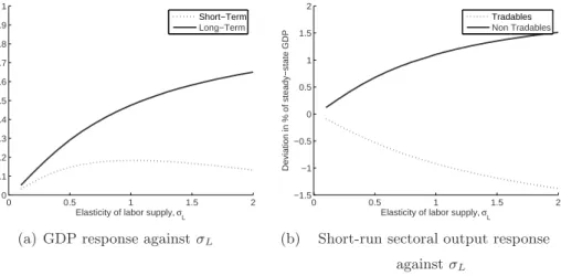
to vary from 0.1 to 2. Figure 3(a) plots both the long-run and initial response of GDP against

σL while Figure 3(b) plots both traded and non traded output impact responses against the

sensitivity of labor supply.

As illustrated in Figure 3(a), like Baxter et King [1993] who use a one-sector model, the GDP response in the long-run rises withσL. As labor gets more sensitive to the rise in the

after-tax labor income, the non traded sector experiences a larger labor outflow. The consecutive greater excess of demand for non tradables requires a larger increase in the stock of capital to clear the non traded good market. Yet, unlike Baxter and King [1993], the relationship between the short-run response of GDP and the elasticity of labor supply displays a hump-shaped pattern. This non monotonic relationship can be best understood by using a sectoral decomposition. Interestingly, Figure 3(b) shows that, as labor supply gets more responsive, non traded output rises more whereas traded output declines further. The explanation is as follows. As labor supply is more responsive, the excess of demand in the non traded good market gets larger, so that the relative price of non tradables appreciates more on impact. The larger increase in p raises further YN but lowers YT more. As long as σL > 1, raising labor

supply responsiveness implies that the larger decline in traded output more than offsets the stronger increase in non traded output which results in a smaller rise in GDP, as shown in Figure 3(a).

0 0.5 1 1.5 2 0 0.1 0.2 0.3 0.4 0.5 0.6 0.7 0.8 0.9 1

Elasticity of labor supply, σ_L

Deviation in % of steady−state GDP

Short−Term Long−Term

(a) GDP response againstσL

0 0.5 1 1.5 2 −1.5 −1 −0.5 0 0.5 1 1.5 2

Elasticity of labor supply, σ_L

Deviation in % of steady−state GDP

Tradables Non Tradables

(b) Short-run sectoral output response againstσL

Figure 3: Sensitivity of Output Responses to Labor Supply Responsiveness

6

Endogenous Markups and Sectoral Effects of Tax Reforms

Recently, several papers have stressed that the variation in the number of competitors and the consecutive change in the markup provides an important magnification mechanism, see e.g. Jaimovich and Floetotto [2008], Wu and Zhang [2000], Zhang [2007] who consider one-sector models. We thus investigate the sectoral effects of tax reforms by allowing for the markup to be endogenous.27

6.1 Steady-state Effects

So far, we adopted the Dixit-Stiglitz assumption according to which the number of competitors is large enough within each sector to yield a fixed price-elasticity of demand. Yet, as emphasized by Yang and Heijdra [1993], the assumption of Dixit and Stiglitz [1977] is an approximation when the final good is aggregated by a finite number of intermediate goods. We depart from the usual practice, following Gal´ı [1994], in assuming that the number of firms is large enough so that we can ignore the strategic effects but not so large that the effect of entry is minuscule on the firm’s demand curve. Consequently, the price elasticity of demand faced by a single firm is no longer constant and equal to the elasticity of substitution between any two varieties, but rather a function of the number of firms N. Taking into account that output of one variety does not affect the general price indexp, but influences the sectoral price level, in a symmetric equilibrium, the resulting price elasticity of demand writes as:28

e(N) =²−(²−ω)

N , N ∈(1,∞). (22)

Assuming that ² > ω, the price elasticity of demand faced by one single firm is an increasing function of the number of firmsN within a sector. Henceforth, the markupµ= _e−e₁ decreases

27_{We assume that the traded sector is more capital intensive than the non traded sector for clarity purpose.}

Numerical results for the casekN _{> k}T _{are available upon request.} 28_{Details of derivation can be found in the Appendix.}