The effects of variable viscosity and thermal conductivity on mhd flow due to a point sink

(1)

c

Escuela Regional de Matemáticas Universidad del Valle - Colombia

Mira Choudhury

N. N. S. College

Gopal Chandra Hazarika

Dibrugarh University

Received Apr. 4, 2006 Accepted Oct. 9, 2006

Abstract

A theoretical investigation of the influence of variable viscosity and thermal conductivity on the MHD boundary layer flow due to a point sink is presented. Both the fluid viscosity and thermal conductivity are assumed to vary as inverse linear functions of temperature. The flow governing partial differential equations are transformed into ordinary differential equations by means of similarity transformation. The problem is solved numerically using shooting method .The effects of viscosity parameter, thermal conductivity parameter and magnetic field parameter on the flow

field forPr= 0.70andEc= 0.10are considered. From the results it has been observed that the

effects of the above variable thermo-viscous parameters and magnetic parameter are considerable and they have to be taken into consideration in the flow and heat transfer problem.

Keywords: MHD Flow, Variable Viscosity, Variable Thermal Conductivity, Point Sink.

MSC(2000): Primary 76 D, Secondary 76N20,76W05.

1 Introduction

Most of the research works had been done on laminar flow and convective heat transfer under the influence of thermo physical properties owing to its application in technological fields and most previous investigations have considered constant physical properties of ambient fluid. But temperature dependent physical prop-erties like viscosity of the fluid and thermal conductivity play a significant role in fluid mechanics. Herwig and Gerstein (1986),Ling and Dybbs (1987), Lai and

Kulacki (1990), Pop.I, et.al (1992), Eswara and Nath (1994), Eswara and

Bom-maih (2000) established that temperature dependent viscosity has a pronounced effect on momentum and thermal transport in the boundary layer region. To accurately predict the flow and the heat transfer rate it is necessary to take into account the variation of viscosity. Problems of this type have important appli-cations in geophysics particularly geothermal energy extraction and underground storage system.

The study on the effects of thermal conductivity variation on heat transfer problems is also vary important to have the more accurate picture of the thermal transport. Khound and Hazarika (2000) observed that a significant variation of velocity distribution and temperature distribution take place with the variation of viscosity parameter and thermal conductivity parameter.

On the other hand, in view of increasing technological applications using mag-neto hydrodynamic effect, it is desirable to extend many of the available viscous

(2)

hydrodynamics solutions to include the effects of magnetic field for those cases when the viscous fluid is electrically conducting.

The aim of the present paper is to investigate the effects of variable viscosity and thermal conductivity on a steady axisymmetric boundary layer flow inside a cone due to a point sink in presence of transverse magnetic field fixed to the fluid. The fluid viscosity and thermal conductivity are taken as inverse linear functions of temperature. The boundary layer flow past a cone is relevant to the two-dimensional flow past a wedge [9].

2 Mathematical analysis

Consider the steady laminar axisymmetric flow of a viscous incompressible elec-trically conducting fluid inside a cone at rest with a hole at the vertex of the cone in presence of uniform transverse magnetic field. In order to treat the bound-ary layer flow due to the presence of the hole, the hole is regarded as a three dimensional point sink [9]. In the light of Eswara and Bommaih, the cone has been taken as semi infinite in length so that it can be regarded as independent of

length r. The electrical conductivity of the fluid is assumed to be small so that

the induced magnetic field can be neglected in comparison of applied magnetic field. The viscous dissipation in the energy equation is taken into consideration. The fluid properties are assumed to be isotropic and constant except for the fluid viscosity and thermal conductivity.

Following Lai and Kulacki [6] the fluid viscosity is assumed to be inverse linear function of temperature as 1 µ = 1 µ_∞[1 +γ(T −T∞)] (1) 1 µ =α(T−Tr) (2) a= γ µ_∞, Tr=T∞− 1 γ (3)

where µ = coefficient of dynamic viscosity, µ_∞= coefficient of viscosity at free

stream, γ= a constant based on thermal property of the fluid, a and Tr are

constants and their values depend on the reference state and thermal property of the fluid. In generala >0for liquids and a <0 for gases.

Forγ−→0, µ=µ_∞ (constant).

(3)

Hazarika [5]): 1 k = 1 k_∞[1 +ξ(T−T∞)] (4) 1 k =c(T−Tk) (5) c= ξ k_∞, Tk=T∞− 1 ξ (6)

where k = thermal conductivity of the fluid, k_∞ = thermal conductivity of the

fluid at free stream, c and Tk are constants and their values depend on the

ref-erence state and thermal property of the fluid ξ, a constant based on thermal

property of the fluid. c >0for liquids and c <0 for gases. The flow governing equations for the present problem are

∂(ru) ∂u + ∂(rw) ∂z = 0 (7) u∂u ∂r +w ∂u ∂z =U ∂U ∂r + 1 ρ_∞ ∂ ∂z µ∂u ∂z −σB 2 0 ρ_∞ u (8) u∂T ∂r +w ∂T ∂z = 1 ρ_∞ ∂ ∂z k∂T ∂z + 1 ρ_∞cp µ ∂u ∂z 2 (9) whereuandware the radial and axial velocities in the directions ofr andz,σ is the electrical conductivity,ρ_∞is the density at free stream, T is the temperature,

cp is the specific heat, B0 is the applied magnetic field strength, U is the free

stream velocity.

The main stream flow is given by

U =₋m

r2 (10)

wherer = distance measured along the cone from the vertex,

m = strength of the point sink,m >0. The boundary conditions are:

z_−→0, u= 0, w= 0, T =Tw (11)

z_{−→ ∞}, u=U, T =T_∞

Tw =temperature at the wall,

T_∞=temperature at the free stream.

We introduce the stream function ψ defined by

ru= ∂ψ

∂z, rw=− ∂ψ ∂r

and a dimensionless stream functionf(η) to obtain velocity profile by

(4)

where η= m 2νr3 1 2 z, (13)

η being the similarity variable, ν = µ_ρ kinematic viscosity,ρ=density of the fluid. Using the transformation

u=U f0(η), w=mν

2r3 1

2

f −3ηf0 (14)

and the dimensionless function for temperature θ(η) = T−T∞ Tw−T∞

, (15)

the continuity equation is identically satisfied and the momentum and heat trans-fer equations reduce to

f000+ 1− θ θr {4(1−f02)₋f f00+ 2M f0_}+ f00θ0 θr−θ =0 (16) 1 Pr θ00− θ0 2 θ₋θk −f θ0+Ecf002=0 (17)

The transformed boundary conditions are

η= 0;f0= 0, θ= 1, f = 0, η_{−→ ∞};f0= 1, θ= 0. (18) where θr = Tr−T∞ Tw−T∞ =₋ 1 γ(Tw−T∞)

is a viscosity measuring parameter ranging from -10 to +10 which is positive for

gases and negative for liquids whenTw−T∞ is positive.

θk = Tk−T∞ Tw−T∞ =− 1 ξ(Tw−T∞) ,

transformed dimensionless reference temperature corresponding to thermal con-ductivity parameter. Pr= ν K Prandtl number, M = σB2₀r ρ_∞U Magnetic parameter, Ec= U2 cp(Tw−T∞) Eckert number, K=Thermal diffusivity.

The above boundary layer approximation is not valid in the immediate neighbor-hood of the hole where, in any case, the main- stream flow cannot represent an actual flow through a hole of small but finite diameter (Roseanhead).

(5)

The physical quantities of interest of this problem are the Skin-friction

coeffi-cient Cf and the Nusselt number Nu which are defined by

Cf = 2τw ρU2 = 2 1/2 θr 1₋θr R−_e1/2f0(0) (19) where τw=µ ∂u ∂z z=0

is the shear stress at the wall, and N u= rqw k(Tw−T∞) =−2 −1/2 θk θk−1 R1_e/2θ0(0) (20) where qw=−k ∂T ∂z z=0

is the heat transfer rate at the wall.

3 Numerical results and discussion

The system of differential equations (16) and (17) governed by the boundary conditions (18) is solved numerically using sho-oting method (9). Numerical cal-culations are carried out for fluids having Prandtl number of 0.70 for various values ofθr, θk, M, and Ec= 0.10.

Various missing values for the solutions of the equations (16), (17), (18) are tabulated in Table 1, Table 2, Table 3 for different values of θr, θk, M

respec-tively.

Tabla 1:

Missing values for different θr and P r= 0.70,Ec= 0.10,M = 0.50, θk=−12 θr f00(0) −θ0(0) -12 2.600774 0.493748 -10 2.623146 0.492431 -8 2.656302 0.49048 -6 2.710533 0.487292 -4 2.81541 0.48114 -2 3.105856 0.464218 Tabla 2:

Missing values for differentθk and P r= 0.70,Ec= 0.10,M = 0.50, θr=−10 θk f00(0) −θ0(0) -15 2.623051 0.488075 -14 2.623078 0.489324 -12 2.623147 0.492431 -10 2.623241 0.496742 -8 2.623381 0.503127 -6 2.623608 0.513559 -4 2.624043 0.533683 -2 2.625219 0.588964 Table 1 shows that f00(0) increases whileθ0(0) decreases with the increase in θr. From the equations (19) and (20) it is quite clear that there is a substantial

(6)

Figure 1: (left) Variation of Velocity Profiles, (right) Variation of Temperature Profiles forPr= 0.7, M = 0.50, Ec = 0.1, θk =−12

1

Fig.1. (a) Fig.1. (b)

Fig. 1.(a) Variation of Velocity Profiles, (b) Variation of Temperature Profiles for Pr = 0.7, M =0.50, Ec = 0.1, θk= -12.

Fig.2. (a) Fig.2. (b)

Fig.2. (a) Variation of Velocity Profiles, (b) Variation of Temperature Profiles for Pr=0.7,

Ec =0.10, θr =-10,θk =-12. 0 0.2 0.4 0.6 0.8 1 1.2 0 0.5 1 1.5 2 M=0.0 M=1.0 M=2.0 M=3.0 0 0.2 0.4 0.6 0.8 1 1.2 0 0.5 1 1.5 2 θr =-15 θr =-10 θ_r =-5 θ_r_=-2 η f'(η ) 0 0.2 0.4 0.6 0.8 1 1.2 0 0.5 1 1.5 2 η θ(η) θr =-15 θr =-10 θr =-5 θr =-2 0 0.2 0.4 0.6 0.8 1 1.2 1.4 1.6 1.8 0 0.5 1 1.5 2 η f'(η) M=0.0 M=1.0 M=2.0 M=3.0 θ(η) η 1

Fig.1. (a) Fig.1. (b)

Fig.2. (a) Fig.2. (b)

Fig.2. (a) Variation of Velocity Profiles, (b) Variation of Temperature Profiles for Pr=0.7, Ec =0.10, θr =-10,θk =-12. 0 0.2 0.4 0.6 0.8 1 1.2 0 0.5 1 1.5 2 M=0.0 M=1.0 M=2.0 M=3.0 0 0.2 0.4 0.6 0.8 1 1.2 0 0.5 1 1.5 2 θr =-15 θr =-10 θ_r_=-5 θr =-2 η f'(η ) 0 0.2 0.4 0.6 0.8 1 1.2 0 0.5 1 1.5 2 η θ(η) θr =-15 θ_r_=-10 θr =-5 θr =-2 0 0.2 0.4 0.6 0.8 1 1.2 1.4 1.6 1.8 0 0.5 1 1.5 2 η f'(η) M=0.0 M=1.0 M=2.0 M=3.0 θ(η) η

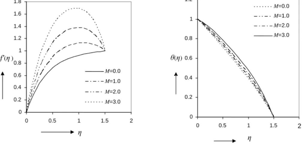
Figure 2: (left) Variation of Velocity Profiles, (right) Variation of Temperature Profiles forPr= 0.7, Ec= 0.10, θr=−10, θk =−12.

1

Fig.1. (a) Fig.1. (b)

Fig.2. (a) Fig.2. (b)

Fig.2. (a) Variation of Velocity Profiles, (b) Variation of Temperature Profiles for Pr=0.7, Ec =0.10, θr =-10,θk =-12. 0 0.2 0.4 0.6 0.8 1 1.2 0 0.5 1 1.5 2 M=0.0 M=1.0 M=2.0 M=3.0 0 0.2 0.4 0.6 0.8 1 1.2 0 0.5 1 1.5 2 θr =-15 θ_r_=-10 θr =-5 θr =-2 η f'(η ) 0 0.2 0.4 0.6 0.8 1 1.2 0 0.5 1 1.5 2 η θ(η) θ_r=-15 θr =-10 θr =-5 θ_r_=-2 0 0.2 0.4 0.6 0.8 1 1.2 1.4 1.6 1.8 0 0.5 1 1.5 2 η f'(η) M=0.0 M=1.0 M=2.0 M=3.0 θ(η) η 1

Fig.1. (a) Fig.1. (b)

Fig.2. (a) Fig.2. (b)

Fig.2. (a) Variation of Velocity Profiles, (b) Variation of Temperature Profiles for Pr=0.7, Ec =0.10, θr =-10,θk =-12. 0 0.2 0.4 0.6 0.8 1 1.2 0 0.5 1 1.5 2 M=0.0 M=1.0 M=2.0 M=3.0 0 0.2 0.4 0.6 0.8 1 1.2 0 0.5 1 1.5 2 θr =-15 θ_r =-10 θ_r_=-5 θr =-2 η f'(η ) 0 0.2 0.4 0.6 0.8 1 1.2 0 0.5 1 1.5 2 η θ(η) θr =-15 θr =-10 θr =-5 θr =-2 0 0.2 0.4 0.6 0.8 1 1.2 1.4 1.6 1.8 0 0.5 1 1.5 2 η f'(η) M=0.0 M=1.0 M=2.0 M=3.0 θ(η) η

Figure 3: (left) Variation of Velocity Profiles, (right) Variation of Temperature Profiles forPr= 0.7, Ec= 0.10, θr=−10, M= 0.50.

1

Fig.3. (a) Fig.3. (b)

Fig.3. (a) Variation of Velocity Profiles, (b) Variation of Temperature Profiles for Pr=0.7, Ec =0.10, θr =-10,M =0.50. 0 0.2 0.4 0.6 0.8 1 1.2 0 0.5 1 1.5 2 η θ(η) θk=-15 θk=-10 θk=-5 θk=-2 0 0.2 0.4 0.6 0.8 1 1.2 0 0.5 1 1.5 2 η f'(η) θk=-15 θk=-10 θk=-5 θk=-2 1

Fig.3. (a) Fig.3. (b)

Fig.3. (a) Variation of Velocity Profiles, (b) Variation of Temperature Profiles for Pr=0.7, Ec =0.10, θr =-10,M =0.50. 0 0.2 0.4 0.6 0.8 1 1.2 0 0.5 1 1.5 2 η θ(η) θk=-15 θk=-10 θk=-5 θk=-2 0 0.2 0.4 0.6 0.8 1 1.2 0 0.5 1 1.5 2 η f'(η) θk=-15 θk=-10 θk=-5 θk=-2

(7)

M f00(0) −θ0(0) 0 2.399705 0.520559 0.5 2.623146 0.492431 1 2.88099 0.457579 1.5 3.176964 0.4145 2 3.514143 0.36155 2.5 3.894627 0.297025 3 4.319348 0.219262

Table 3: Missing values for differentM andP r= 0.70,Ec= 0.10,θk =−12,θr=−10 variation in Skin friction coefficient and heat transfer rate. This variation is significant in case of Cf. Table 2 shows that values off00(0) and -θ0(0)increases

with the increase in θk. It is seen that variation f00(0)with θk is less significant

compare to that with θr. Table 3 indicates that other parameters remaining

same, skin fiction coefficient increases and the heat transfer rate decreases with

the increasing values of of M. This variation is much more significant.

Fig.1. display the velocity and temperature distribution respectively within

the boundary layer for Pr = 0.70, M = 0.5, Ec = 0.10 and θk = −12 with

the variation ofθr. It is observed that velocity boundary layer increases with the

increase ofθr. But the effect of viscosity variation parameterθris not so prominent

in case of thermal boundary layer. Fig.2. depict the effects of the magnetic field on velocity and temperature profile. It is observed that velocity boundary layer increases tremendously in presence of magnetic field. Fig.3. (right) displays the variation of temperature profile with the variation of thermal conductivity

parameter θk. It is observed that thermal boundary layer decreases with the

increasing values of thermal conductivity parameter θk. Fig.3.(left) shows that

velocity variation against θk is not so prominent.

4 Conclusion

The above analysis shows that the viscosity variation parameter, thermal con-ductivity parameter and magnetic parameter has substantial effect on velocity field and temperature field as well as on the drag and heat transfer characteristic within the boundary layer due to a point sink.

Acknowledgements The authors are thankful to Prof. B. S. Bhatt, The Uni-versity of West Indies, West Indies, for his valuable suggestions.

References

[1] Conte, S.D., Boor,Carl De: Elementary Numerical Analysis: An Algorithmic Approach., 3rd edition, 6th print, McGraw Hill international Book Company, London. (1983).

(8)

[2] Eswara, A.T. and Bommaih, B.T.: The effect of variable viscosity on laminar flow due to a point sink, Indian J. pure and appl. Math., 35 (6), (2004),pp.811-815.

[3] Eswara, A.T. and Nath, G.:Unsteady non-similar two dimensional and ax-isymmetric water boundary layer with variable viscosity and Prandtl number., Int.J. Engg.Sc., Vol 32, (1994), pp. 267 - 279.

[4] Herwig, H .and Gerstein, K.: Warm and Staffbertr.: 20 (1986), pp. 47 . [5] Khound,P.K. and Hazaika,G.C.: The effect of variable viscosity and thermal

conductivity on liquid film on an unsteady stretching surface., Proc.of 46th Annual Tech.Session, Ass.Sc.Soc. (2000),pp.47 - 56.

[6] Lai, F. C. and Kulacki, F. A.: The effect of variable viscosity on convective heat transfer along a vertical surface in a saturated porous medium. Int. J. Heat Mass Transfer, 33, (1990), pp.1028 - 1031.

[7] Ling, J.X.and Dybbs, A.: Forced convection over a flat plate submerged in a porous medium, variable viscosity case, ASME paper 87 -WA /HT -23 New York (1987).

[8] Pop, I., Gorla,R.S.R. and Rashid,M.: The effect of variable viscosity on flow and heat transfer to a continuous moving flat plate., Int. J. Engg. Sc., Vol 30 No.1, (1992), pp.1- 6.

[9] Roseanhead, (Ed.) Laminar Boundary Layer, Oxford University Press, Ox-ford, (1963), p. 427.

Authors’ address

Mira Choudhury — N. N. S. College, Department of Mathematics, Titabar, Assam -785630, India

e-mail: [email protected]

Gopal Chandra Hazarika — Department of Mathematics, Dibrugarh University, Dibru-garh, Assam-786004, India.