Munich Personal RePEc Archive
Do Intergovernmental Grants Improve
Public Service Delivery in Developing
Countries?
Cassidy, Traviss
University of Alabama
1 September 2017
Online at
https://mpra.ub.uni-muenchen.de/104250/
Do Intergovernmental Grants Improve Public Service
Delivery in Developing Countries?
*Traviss Cassidy
†First version: September 2017
This version: November 2020
Abstract
I exploit unusual policy variation in Indonesia to examine how local responses to intergovernmental grants depend on their persistence. A national reform produced permanent increases in the general grant that were larger for less densely populated districts. Hydrocarbon-rich districts experienced transitory shocks to shared resource revenue. Public service delivery strongly responded to the permanent shock, but not to the transitory shocks, consistent with districts providing lumpy public services as a function of lifetime fiscal resources. I provide supporting evidence for this mechanism and rule out other potential mechanisms. I discuss implications for decentralization policy and research on taxation and accountability.
JEL codes: H72, H75, H77, O13, Q38
Keywords: Intergovernmental grants, public goods, flypaper effect, resource curse
*I thank David Agrawal, David Albouy, Martín Besfamille, Chris Blattman, Hoyt Bleakley, Will Boning, Anne
Brockmeyer, Alecia Cassidy, Connor Cole, Jim Cust, Mark Dincecco, François Gerard, Diana Greenwald, Steve Hamilton, Jim Hines, Brad Humphreys, Byung-Cheol Kim, Shin Kimura, Joana Naritomi, Ricardo Perez-Truglia, Pablo Querubín, Monica Singhal, Joel Slemrod, Ugo Troiano, Tejaswi Velayudhan, Dean Yang, and seminar participants at the University of Michigan at Ann Arbor, University of Michigan at Dearborn, Northwestern University, Office of Tax Analysis at the U.S. Department of the Treasury, George Washington University, University of Illinois at Urbana-Champaign, University of Wyoming, Florida International University, University of Alabama, National Tax Association Annual Conference, Southern Economic Association Annual Conference, and International Institute of Public Finance Annual Congress for helpful comments. I am grateful to Monica Martinez-Bravo and Andreas Stegmann for generously sharing data. I thank Lauren Johnson for excellent research assistance. I gratefully acknowledge financial support from the University of Michigan Rackham Graduate School and the Michigan Institute for Teaching and Research in Economics (MITRE) Anonymous Donor, and research support from the University of Michigan Library. A previous version of this paper was circulated with the title, “How Forward-Looking Are Local Governments? Evidence from Indonesia.”
1 Introduction
Citizens perceive the granting of intergovernmental fiscal transfers as the magical art of passing money from one government to another and seeing it vanish into thin air. These perceptions are well grounded in reality in developing countries . . .
(Shah,2006, p. 17)
Intergovernmental transfers play an outsized role in local public finance in developing countries, yet many policymakers and academics are skeptical that increasing transfers to local governments will improve public service delivery. Supporting this skepticism are well-documented cases of local officials misappropriating funds from the center (e.g.,Reinikka
and Svensson,2004;Olken,2007;Ferraz and Finan,2008,2011) and several studies showing
that transfers reduce the quality of governance and fail to stimulate greater public good provision in Latin America.1 The debate is far from over, however. Measurement issues make it difficult to prove that funds have not been put to good use,2and some studies have found positive impacts on public service delivery (Litschig and Morrison,2013;Olsson and
Valsecchi,2015).
This paper identifies and addresses a novel empirical challenge: when local governments are forward-looking, the responses of public services to transitory changes in fiscal transfers do not reflect the true contribution of these funds to public service delivery. Governments that optimize intertemporally recognize that transitory changes in volatile transfers, such as shared natural resource revenue, have a relatively small impact on the intertemporal budget constraint. Increases in this type of transfer thus may not stimulate investment in new structures or hiring of frontline workers. Researchers may then mistakenly conclude that the funds are wasted or stolen, even when local officials are scrupulous. On the other hand, responses to permanent changes in transfers are highly informative for the marginal contribution of these funds to public service delivery.
I exploit unusual policy variation in Indonesia to study local government responses to two intergovernmental transfers of varying persistence. District governments are responsible for providing public goods and services in the areas of education, health, and local infrastructure, which are primarily financed by fiscal transfers. The country’s largest intergovernmental transfer, the general grant, is highly persistent. A change in the allocation formula resulted in permanent increases in this grant that were larger for less densely populated districts. I exploit the sharp increase in the revenue gradient in land area per capita to estimate the causal effects of apermanentincrease in fiscal transfers. The second-largest transfer is the oil
1SeeCaselli and Michaels(2013),Brollo, Nannicini, Perotti, and Tabellini(2013),Monteiro and Ferraz(2014),
andGadenne(2017) on Brazil, and seeMartínez(2020) on Colombia.
2Local governments can spend funds on a variety of projects and can invest in quality improvements that are
not captured in available datasets. Some researchers have confronted these challenges by using detailed data on a wide array of public goods and services, and by examining outcomes, such as education or income, that should respond to quality improvements (e.g.,Caselli and Michaels,2013;Litschig and Morrison,2013).
and gas grant, which is tied to local hydrocarbon extraction and exhibits significant transitory variation in hydrocarbon-rich areas. I exploit the central government’s royalty-sharing rule, spatial variation in initial hydrocarbon endowments, and time-series variation in aggregate revenue from this grant to estimate the causal effects oftransitoryshocks to fiscal transfers. The permanent increase in the general grant stimulated greater provision of public schools, health facilities and personnel, and local roads. Increasing the grant by IDR 1 million (approximately USD 100) per capita improved overall public service delivery by half a standard deviation, relative to pre-reform levels. By contrast, transitory shocks to the oil and gas grant had small and statistically insignificant effects, and the estimates are precise enough to rule out moderate increases in public service delivery. For most outcomes we can statistically reject equal responses to the two grants, even after adjusting for multiple hypothesis testing.
The results are consistent with a model in which local governments provide lumpy public goods and services as a function of lifetime fiscal resources. The mean-reverting nature of the oil and gas grant implies that current-year changes have a small impact on lifetime resources. Even if the government has a high discount rate, it will be hesitant to increase spending on structures such as schools, which require a large upfront investment and a future stream of maintenance expenditure, or on employees that enjoy significant job security, when oil and gas revenue increases. Holding fixed the size of the initial revenue shock, more persistent increases in revenue are more likely to stimulate large investments and hiring sprees.
Supporting this mechanism, the expenditure response to the general grant is hump-shaped over time and overshoots at its peak, increasing by about 1.60 rupiah for every rupiah of revenue, indicating large upfront investments. Hydrocarbon-rich districts do not perfectly smooth their spending, but the expenditure response to the oil and gas grant is around one third of the response to the general grant. Furthermore, the gap in the responses is smaller for more discretionary and less lumpy categories of spending, and larger for capital and personnel expenditure.
I consider other potential mechanisms for the results. One possibility is that the magnitude of the grant shocks differ, and responses are nonlinear in the size of the current-year shock. Another possibility is that districts respond asymmetrically to increases and decreases in transfers. I test for these two mechanisms and find little evidence that they drive the results. I also find little evidence that the differential effects of the grants operate through changes in political competition. Alternatively, the oil and gas grant may be more susceptible to waste or embezzlement, even though the grants are formally subject to the same rules and oversight by the central government. If this were true, then permanent increases in the oil and gas grant should stimulate public service delivery much less than permanent increases in the general grant. I test this theory by exploiting the increase in permanent oil and gas grant revenue induced by Indonesia’s decentralization in 2001. Using this source of variation, I find economically and statistically significant increases in public service delivery that are in the
same ballpark as the increases induced by the general grant. Although waste and corruption are common in district governance, they cannot explain a significant portion of thedifference
in the responses to the two grants over the post-decentralization period.
Besides unique policy variation, the Indonesian setting offers additional advantages. First, there are a large number of district governments—over 300—with broad spending authority in the areas of education, health, and infrastructure. Second, national regulations deprive district governments of any control over income-tax or property-tax policy. This eliminates an important margin of response to revenue shocks—tax cuts—and enables the analysis to isolate the decision of how much to spend rather than save, and when to spend. Third, rich data on district fiscal outcomes and public service delivery over 1999–2014 make it possible to examine dynamic responses to fiscal transfers along many margins.
The results are informative for decentralization policy around the world. International organizations have pushed for greater fiscal decentralization in the developing world (World
Bank,1999;United Nations,2009), but central governments have generally been hesitant to
devolve tax responsibilities to local governments. Consequently, intergovernmental grants finance around 60 percent of subnational expenditure in developing countries but only around a third of subnational expenditure in OECD countries (Shah,2006). An important question is whether central governments in developing countries should cede more tax authority to subnational governments to strengthen tax-benefit linkages (Gadenne and
Singhal,2014). Knowing how effective fiscal transfers are at achieving their objectives, and
what type of variation in transfers can yield this information, is crucial in this debate. This paper contributes to multiple literatures in development and public finance. First, it contributes to the literature that examines whether intergovernmental transfers actually improve public service delivery. As already mentioned, the evidence in this literature is mixed.3 Motivated by the disappointing performance of some fiscal transfer programs,
Gadenne(2017) andMartínez(2020) examine whether increases in local tax revenue lead
to better outcomes than increases in transfers in Brazil and Colombia, respectively. Both studies conclude that tax revenue stimulates improvements in public service delivery, but transfers do not.4In this literature little attention is paid to the persistence of the revenue shocks used for causal identification, which cannot be summarized by simple measures like the within-unit coefficient of variation. Consequently, it is difficult to know whether the divergent results are due to differences in context, accountability, or revenue persistence.
Second, this paper is related to research on the so-called flypaper effect, the empirical regularity that local governments have a greater propensity to spend out of non-matching
3Caselli and Michaels(2013) andMonteiro and Ferraz(2014) find that shared oil and gas revenue caused
declines in public service delivery in Brazilian municipalities. However,Litschig and Morrison(2013) show that in an earlier period in Brazil, a formula-based, general-purpose transfer improved education outcomes.Olsson and Valsecchi(2015) provide earlier evidence that Indonesia’s oil and gas grant improved public service delivery using a shorter panel and a different empirical strategy.
4In a related study,Borge, Parmer, and Torvik(2015) find that tax revenue and natural resource revenue have
grants than out of local private income.5This research seeks to determine how much grant revenue is spent, and how much is passed on to citizens via lower taxes. By contrast, I focus on the dynamic responses of expenditure and public service delivery in a setting where local governments have no control over tax rates.6 I build on this literature by showing that permanent increases in fiscal transfers induce larger and more immediate expenditure responses than transitory increases.7 Knowing the timing of fiscal responses to grants is important for conducting countercyclical fiscal policy in a federation.
Finally, this research contributes to the literature on the resource curse (van der Ploeg, 2011). One concern in this literature is that the volatility and sheer size of resource-related fiscal transfers will lead to wasteful and volatile local spending (Cust and Viale,2016;Natural
Resource Governance Institute,2016). If this concern is well founded, then central governments
should consider smoothing revenue on behalf of local governments and distributing the funds from resource extraction more evenly across regions. I contribute to this debate by showing that in the context of Indonesia, natural resource revenue and less volatile general-purpose grants promote public service delivery to a similar degree, after properly accounting for the persistence of revenue shocks.
The rest of the paper proceeds as follows. Section2provides background information on institutions and local public finance in Indonesia following the transition to democracy. Section3presents a theoretical model of public expenditure on nondurable and lumpy durable goods in order to highlight how responses can depend on grant persistence and to generate testable predictions. Section4discusses the fiscal responses of districts to the two grants, and Section5discusses the impacts on public service delivery. Section6provides concluding remarks.
2 Decentralization in Indonesia
2.1 Institutional Background
The resignation of Suharto as president of Indonesia in 1998 marked the end of three decades of centralized, authoritarian rule and gave way to democratic reforms and fiscal decentralization. There are four levels of subnational public administration in Indonesia: province, district, subdistrict, and village. Districts are responsible for the bulk of subnational policymaking; provinces mostly play a coordinating role, and subdistricts (kecamatan) carry
5SeeHines and Thaler(1995) andInman(2008) for summaries of the literature. Recent contributions include
Knight(2002),Baicker(2005),Dahlberg, Mörk, Rattsø, and Ågren(2008),Lutz(2010),Gennari and Messina (2014),Vegh and Vuletin(2015),Lundqvist(2015),Dahlby and Ferede(2016), andLiu and Ma(2016).
6Gordon(2004),Cascio, Gordon, and Reber(2013),Leduc and Wilson(2017), andHelm and Stuhler(2020)
also estimate dynamic fiscal responses to grants.
7To the best of my knowledge, the only other paper that compares fiscal responses to two grants with differing
persistence isBesfamille, Jorrat, Manzano, and Sanguinetti(2019), who find qualitatively similar results using data on Argentinian provinces.
out district policies. Districts are categorized as either rural districts (kabupaten) or urban
districts (kota), but both types operate under the same political and fiscal institutions. Starting
in 1999, district parliaments were directly elected through a proportional representation system. The district heads (“mayors”) previously appointed by Suharto were allowed to finish their five-year terms, after which time the local parliament appointed the mayor. Starting in 2005, districts selected the mayor by direct election. Incumbent mayors were allowed to finish their terms before direct elections could be held, resulting in a staggered rollout of direct elections across districts from 2005 to 2008. Mayors can serve at most two five-year terms.
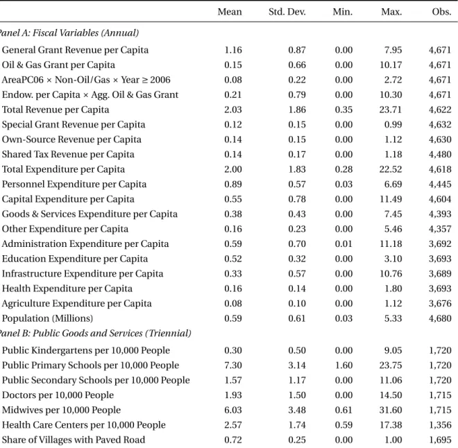
The “Big Bang” decentralization reforms of 2001 devolved significant expenditure authority to districts, so that Indonesia now ranks as one of the most decentralized countries in the developing world (Shah, Qibthiyyah, and Dita,2012). Panel A of Table1summarizes district revenue and expenditure. Districts provide public goods and services in the areas of education, health, and local infrastructure. However, own-source revenue accounts for only seven percent of total district revenue, so public expenditure is primarily financed by intergovernmental grants.8Most local funding comes from an unconditional grant known as the general grant (Dana Alokasi Umum), which accounts for over half of district revenue
on average. A minority of districts receive significant revenue from local natural resource extraction. I discuss these two revenue sources in detail ahead. A small portion of expenditure is financed by earmarked “special grants” (Dana Alokasi Khusus) provided by the central government on a discretionary basis. Districts were prohibited from introducing income or property taxes over the study period, however they received a portion of tax revenue collected by the central government within the district. Shared tax revenue accounts for around seven percent of the district budget.
Following decentralization, subnational borrowing has been minimal, for three reasons. First, the central government banned foreign borrowing by districts and must pre-approve domestic borrowing (Blöndal, Hawkesworth, and Choi,2009). Second, many districts have poor credit ratings. Finally, district governments have had difficulty spending all of their transfer revenue in a timely fashion, leading to a buildup of reserves (World Bank, 2007, pp. 127–128). Current revenue and reserves typically suffice to finance large capital projects and smooth current expenditure.
The number of districts has grown from 341 in 2001 to 514 in 2014, due to district splitting.9 The central government imposed two moratoria on splitting during the analysis period, the first from 2004 to 2006 and the second from 2009 to 2012. As a consequence, no splits occurred in 2006, the year that the general grant and the oil and gas grant experienced their largest shocks, as discussed ahead. Due to the structure of the general grant, transfers typically
8Own-source revenue mostly consists of business license fees, hotel and restaurant taxes, and utility fees. 9SeeFitrani, Hofman, and Kaiser(2005),Burgess, Hansen, Olken, Potapov, and Sieber(2012), andBazzi and
increase in per-capita terms in both the original district and the new district(s) after a split. The baseline regressions flexibly control for district splits, though none of the results are sensitive to controlling for splits.
Indonesia initiated a second wave of decentralization reforms with the 2015 Village Law, which increased the authority of village governments to provide public services and increased fiscal transfers to villages. I focus on the period 2001–2014 to hold the federal structure constant.
2.2 General Grant
As already mentioned, the largest source of financing for most district governments is the General Allocation Fund (Dana Alokasi Umum), or “general grant” for short. The general grant is intended to equalize district capacity to provide local public services.10 Each year the central government sets the total budget for the grant and allocates funds according to a formula. Half of the grant pool funds the “basic allocation,” which covers the civil service wage bill. The basic allocation increases one-for-one with wage costs, but central regulations on recruitment and staffing prevent exorbitant spending on public employees that would otherwise occur due to the structure of the grant (Shah et al.,2012). The remaining half of the general grant pool is allocated according to the “fiscal gap,” which is the difference between expenditure needs and fiscal capacity. Expenditure needs are calculated as a weighted sum of indices related to population, land area, poverty, and construction costs. Fiscal capacity is defined as a weighted sum of imputed own-source revenue, shared tax revenue, and shared natural resource revenue. Appendix SectionA.2provides details on the formulae. After paying civil servant wages, districts have complete discretion over how to spend the grant.
In 2006 the central government dramatically increased the budget for the general grant. The grant budget depends on forecasts of the national government’s long-term budget health, and a key parameter in these forecasts is the assumed future oil price. For years, the central government had deliberately underestimated the oil price to reduce its transfer obligations
(Lewis and Oosterman,2009). Since 1999, the debt-to-GDP had been falling rapidly, creating
space for expanding transfers (World Bank,2007, p. 10). In 2006 the general grant budget increased by 44 percent after the central government increased the oil price assumption from USD 30 per barrel to USD 60 per barrel (Agustina, Ahmad, Nugroho, and Siagian,2012). That same year the central government changed the allocation formula, reducing the weight assigned to population and increasing the weight assigned to land area. The change in general grant revenue per capita dictated by the formula adjustment and budget increase was roughly linear in land area per capita. (See Appendix SectionA.2.) Districts rich in oil and gas resources should have experienced a decline in general grant funds at this time, due
10Equalization grants have the potential to promote equity by targeting areas populated by households with
low earning potential. In real-world contexts, such as in Canada, such grants often distort household location decisions and fall short of equity goals (Albouy,2012).
to a rise in oil and gas revenue. However, a hold-harmless provision froze the general grant allocation in place for these resource-abundant districts (World Bank,2007, p. 121). Both the increase in the budget and the change in the allocation formula were announced in October of 2004 (Law No. 33/2004).
Changes to the grant budget and formula in years other than 2006 were relatively minor, so the reform-driven variation in general grant revenue per capita can be approximated as
Gd,t≈θd+πAd·Nd·1(t≥2006),
whereπ>0, Ad is land area per capita in districtd in 2006, Nd is an indicator for being located in a non-hydrocarbon-rich province, and 1(t≥2006) is an indicator for years 2006 and later.11 The above expression shows that in provinces without significant hydrocarbon endowments, general grant revenue per capita permanently increased in 2006, and the magnitude of the increase was proportional to district land area per capita. Data on district land area and population come from the World Bank’s Indonesia Database for Policy and Economic Research (INDO-DAPOER), and data on intergovernmental grants come from the Ministry of Finance (Kementerian Keuangan). (See Appendix SectionA.4for details.)
Panel (a) of Figure1shows that while less densely populated districts initially received more general grant revenue per capita than more densely populated districts, the gap permanently widened starting in 2006 in non-hydrocarbon-rich provinces. By contrast, in hydrocarbon-rich provinces the gap was roughly constant over time, and there was no permanent increase in the general grant. The policy reform of 2006 therefore created significant cross-district variation in the size of a permanent shock to the general grant within provinces that lack significant oil and gas resources.
The 2006 reform was intended to increase fiscal equalization across regions. There is little indication that political considerations determined the nature of the reform. Conceivably, members of the national legislature representing less densely populated districts could have used the reform to help their own reelection prospects or the prospects of incumbents in the district legislatures. The timing of the reform is inconsistent with this story, however, as elections for both the national and district legislatures took place in 1999, 2004, 2009, and 2014. Alternatively, members of the national legislature may have wanted to improve the reelection prospects of incumbent mayors in less densely populated districts. If this were the case, then one would expect to see a disproportionate number of mayoral elections taking place in these districts in 2006. In reality, among resource-poor provinces, the average land area per capita of districts with mayoral elections in 2006 is statistically indistinguishable from the average land area per capita of districts with mayoral elections in 2005, 2007, or 2008.12This is unsurprising, as the timing of direct mayoral elections was largely determined
11The hydrocarbon-rich provinces are Riau, Kepulauan Riau, Jambi, Sumatera Selatan, and Kalimantan Timur.
(See Appendix FigureA.1.)
by idiosyncratic historical factors (Martínez-Bravo, Mukherjee, and Stegmann,2017). Overall, there is little reason to believe that the timing or size of the general grant reform were motivated by political considerations.
2.3 Oil and Gas Grant
Districts containing natural resources receive Shared Natural Resource Revenue (Dana Bagi Hasil Sumber Daya Alam), which depends on the revenue (royalties and taxes) collected by
the central government from resource extraction within the district and province. Oil and natural gas are by far the largest sources of natural resource revenue in Indonesia. According to the sharing rule, 15.5 percent of oil revenue collected within a district is redistributed to subnational governments: 3.1 percent goes to the provincial government, 6.2 percent goes to the producing district, and the remaining 6.2 percent is evenly divided among the other districts located in the same province. The sharing rule for natural gas is more generous to subnational governments: 6.1 percent goes to the provincial government, 12.2 percent goes to the producing district, and another 12.2 percent is divided equally among the other districts in the province. Despite the less generous sharing rule, shared oil revenue on average exceeds shared gas revenue due to the higher value of oil production. Districts have complete discretion over how to spend the oil and gas grant.13
Using the proprietary Rystad UCube database (Rystad Energy,2016), I calculate the total economically recoverable oil and gas resources in each district as of 2000 (and known in 2000)—prior to fiscal decentralization. I then convert physical endowments into monetary values using the average prices of oil and gas over 2001–2014, insert these variables into the revenue-sharing formula in place of actual oil and gas revenue, and divide by district population. The resulting variable, denoted byEd,t, represents the predetermined oil and gas endowment to which districtdhas a claim for revenue-sharing purposes, in constant 2010 IDR (billions) per capita. Appendix SectionA.3provides more details on the sharing rule and the endowment variable.
Panel (b) of Figure1shows that in districts in the top 5 percent in terms of hydrocarbon endowment, the oil and gas grant was large and experienced sharp year-to-year changes, especially over the period 2005–2009. The oil and gas grant was significantly smaller for districts between the 90th and 95th percentiles of endowment, and virtually nonexistent for districts in the bottom 90 percent. The figure also graphs total oil and gas grant revenue against the weighted value of oil and gas production, where the value of oil production is given a weight of 0.062 and the value of gas production is given a weight of 0.122. The
13In 2009 the central government slightly increased the amount of oil and gas revenue shared with subnational
governments, earmarking this additional revenue for education. As a result, after 2009 around three percent of the district’s oil grant, and two percent of the district’s gas grant, was earmarked. This earmarking is unlikely to play any role in district spending decisions, as earmarked funds are extremely small relative to total education spending, which represents one third of the district budget on average.
weighted value of production should be roughly proportional to the central government’s transfer obligations dictated by the sharing rule. However, the two time series do not track each other—not even with a lag—indicating that the central government varied the timing of grant disbursements on a discretionary basis. The variation in the oil and gas grant driven by resource endowments and central government policies is captured byEd,t·R˜(−d),t, where
˜
R(−d),t is aggregate oil and gas grants excluding own-district grant revenue.14
2.4 Geographic Variation in Exposure to Grant Shocks
The maps in Figure2show the spatial variation in district exposure to shocks to the two grants. Every island group except for Java contains districts with high exposure to the general grant reform—that is, low population density. Furthermore, there is rich within-island variation in land area per capita in all island groups except for Java. Oil and gas endowments are fairly geographically concentrated, with five provinces containing the bulk of the deposits and around one third of districts having an endowment of zero. Nevertheless, there is significant cross-district variation in endowments within most island groups and within hydrocarbon-rich provinces.
2.5 Magnitude and Persistence of Grant Shocks
Both the general grant and oil and gas grant are unconditional, non-matching, and subject to the same level of central-government oversight. Hence, they differ only in their time-series variation. I divide this variation into two components: (1) the initial magnitude of shocks, and (2) the persistence of shocks. To examine the initial magnitude of shocks, Appendix FigureA.2plots the distribution of the absolute two-year change in the general grant during 2005–2007 and the distribution of all absolute two-year changes in the oil and gas grant. In the subsample of districts with high exposure to one of the two grants, these distributions are reasonably similar, and equal in mean. (See Appendix SectionA.5for details.)
Appendix TableA.1presents estimates of persistence based on a dynamic panel model. The GMM estimates of the autoregressive coefficients for the general grant nearly sum to one, implying almost “perfect” persistence. The estimates for the oil and gas grant are less precise, but the totality of the evidence suggests the oil and gas grant is significantly less persistent than the general grant. (See Appendix SectionA.6for details.) The within-district coefficient of variation of the oil and gas grant (1.58) is 5 times that of the general grant (0.32), confirming that the oil and gas grant is more “volatile” than the general grant. However, this measure does not capture the persistence of shocks.15
14Excluding own-district oil and gas grant revenue from the calculation of aggregate oil and gas grants avoids a
potential source of bias in the event that district oil and gas grant revenue is endogenous. Including own-district oil and gas grant revenue in the calculation makes little difference for the estimates, however, as the number of districts is large and no district accounts for more than 10 percent of total oil and gas revenue.
3 Theoretical Model
This section develops a simple model of public expenditure, building on Obstfeld and
Rogoff(1996, pp. 96–98). The goal is to understand how public good provision responds to
revenue shocks of differing persistence, and how lumpy investment affects these responses. Suppose the local government provides a nondurable good,C, and a durable good,D. The durable good evolves according to the equation of motionDt=(1−δ)Dt−1+It, whereIt is durable-good investment in periodt, andδ∈(0,1) is the depreciation rate. Letpt denote the (exogenous) price of durable-good investment in units of the nondurable good in periodt. Total government spending in periodtisGt≡Ct+ptIt. The local government has access to a risk-free bond with exogenous rate of returnr. Fiscal transfers from the central government, Ft, are the local government’s only source of revenue. Net assets,At, evolve according to the equation of motionAt+1=(1+r)At+Ft−Ct−ptIt. The local government’s intertemporal budget constraint is ∞ X t=0 µ 1 1+r ¶t (Ct+ptIt)=(1+r)A0+ ∞ X t=0 µ 1 1+r ¶t Ft.
The government discounts citizen utility over time with factorβ∈(0,1). The government may be impatient, in that its discount rate may be greater than the interest rate (β<1/(1+r)). Initially assume that investment is frictionless (non-lumpy). The government has perfect foresight and chooses a sequence {Ct,Dt}∞t=0to maximize
∞ X t=0 βt¡γlogCt+(1−γ)logDt ¢ ,
subject to the intertemporal budget constraint and the equation of motion for durables.16 Letγ∈(0,1) so that the citizen wants to consume both goods.
The optimal path of public good provision is characterized by the equations
Ct+1=β(1+r)Ct, (1−γ)Ct γDt =pt− 1−δ 1+rpt+1≡ιt. (1)
The first is the usual Euler equation for consumption of nondurables, and the second states that the marginal rate of substitution between nondurables consumption and durables
equalsµ−1 in the first two periods andµ+1 in the last two periods for all districts. The second grant alternates
betweenµ−1 andµ+1 in each period for all districts. The within-unit coefficient of variation is the same for
both grants.
16The model abstracts from private consumption in order to focus attention on the government’s optimal
expenditure plan. As there is no taxation in the model, adding private consumption would not change any of the results below as long as citizen preferences for private consumption and public consumption were separable.
consumption equals the user cost of durables. Define the stock of lifetime resources, R=(1+r)A0+(1−δ)p0D−1+ ∞ X t=0 µ 1 1+r ¶t Ft.
Combining the optimality conditions with the intertemporal budget constraint yields the optimal levels of public good provision in each period,
Ct=βt(1+r)tγ(1−β)R, Dt= 1
ιt
βt(1+r)t(1−γ)(1−β)R.
Next consider how public good provision responds to revenue shocks. Suppose transfers evolve deterministically according to the difference equation
Ft=ρFt−1+ψt,
whereρ∈[0,1] measures the persistence of the transfer. The effect of shockψt on transfers
j periods later is∂Ft+j/∂ψt =ρj. In particular, a one-unit increase inψ0causes transfers
to increase by one in all periods ifρ=1 (permanent increase), but it causes only period-0 transfers to increase by one ifρ=0 (transitory increase). The effect of a period-0 revenue shock on lifetime resources is∂R/∂ψ0=(1+r)/(1+r−ρ), so the response of public good provision in periodtis ∂Ct ∂ψ0 =βt(1+r)tγ(1−β) 1+r 1+r−ρ, ∂Dt ∂ψ0 = 1 ιt βt(1+r)t(1−γ)(1−β) 1+r 1+r−ρ. (2)
The above expressions immediately imply the following result.
Proposition 3.1 The public goods response to a revenue shock is increasing in the persistence
of the shock:
∂2Ct
∂ρ∂ψ0>0,
∂2Dt
∂ρ∂ψ0>0 for all t.
Proposition 3.1 holds because more persistent shocks have a larger impact on lifetime resources.
BecauseDt−1is predetermined in periodt, the initial investment response equals the initial durables response, while the investment response in subsequent periods reflects the change in durables net of depreciation,
∂I0 ∂ψ0 =∂D0 ∂ψ0, ∂It ∂ψ0 =∂Dt ∂ψ0 −(1−δ)∂Dt−1 ∂ψ0 fort ≥1. (3)
Absent a steep downward trend in the user cost of durables over time, investment responds more in the current period than in subsequent periods, as does total government expenditure—
even when the government’s discount rate equals the interest rate.17Together, the expressions in (2) and (3) imply the following result.
Proposition 3.2 For any discount factorβ≤(1+r)−1, total expenditure “overshoots,”
∂G0
∂ψ0
> r 1+r−ρ,
initially increasing by more than the increase in permanent income (r R/(1+r)) due to the shock.18 In particular, if transfers are perfectly persistent (ρ=1), then spending initially increases more than one-for-one with current transfers (∂G0/∂ψ0 > 1). In addition, the
spending response is always smaller in subsequent periods,
∂Gt
∂ψ0
<∂G0
∂ψ0 for t
≥1,
as long as a weak condition holds for the path of investment costs.19
To summarize, when investment is non-lumpy, the expenditure response to a shock to fiscal transfers (1) is larger the more persistent are transfers and (2) initially overshoots under mild assumptions, due to upfront investment in durables.
Now suppose that investment is lumpy due to non-convex adjustment costs. The local government incurs a fixed costξ>0 every time it makes a “large” adjustment to the stock of durables. FollowingKhan and Thomas(2008), the government does not pay this fixed cost if adjustment is sufficiently small relative to the stock of durables—formally, if It ∈ [aDt−1,bDt−1], wherea≤0≤b. An example of such an investment is routine maintenance.
To simplify the dynamics of the model, assume that the price of investment is constant,
ιt =ιfor allt. Further assume that the government’s discount rate equals the interest rate (β(1+r)=1). Under these two assumptions the desired provision of the two public goods is
17Fort≥1, ∂I0 ∂ψ0 − ∂It ∂ψ0 =(1−γ)(1−β)(1+r) 1+r−ρ µ1 ι0 −βt−1(1+r)t−1 ·β(1+r) ιt − 1−δ ιt−1 ¸¶
18To see this, note that
∂G0 ∂ψ0 =(1−β)(1+r) 1+r−ρ µ γ+(1−γ)p0 ι0 ¶ , andp0>ι0as long as the price of investment is always strictly positive.
19Because ∂Gt ∂ψ0 =βt(1+r)t(1−β)(1+r) 1+r−ρ µ γ+(1−γ) · pt ιt − 1−δ β(1+r) pt ιt−1 ¸¶ ,
constant over time and equal to Ct =C=γ r 1+rR, Dt=D= 1−γ ι r 1+rR for allt.
Finally, assume thatb=δso that the government can maintain a constant stock of durables
without incurring the fixed cost. Regardless of whether these three assumptions are imposed, the investment response to a revenue shock will be concentrated in the initial period. The simplifying assumptions make it easier to analyze how non-convex adjustment costs affect this investment response.
For a period-0 shock of size dψ0, let dR=dψ0(1+r)/(1+r−ρ) denote the change in
lifetime resources. If the government does not incur the fixed cost, public good provision is
C=γ r 1+rR+ r 1+rdR, D= 1−γ ι r 1+rR.
The shock leaves the stock of durables unchanged, and all additional resources are devoted to the nondurable good. If the government does incur the fixed cost, the public goods increase proportionally with the increase in lifetime resources, net of the fixed cost:
C=γ r 1+r(R+dR−ξ), D= 1−γ ι r 1+r(R+dR−ξ).
Let dfR denote the change in lifetime resources for which the government is indifferent
between incurring the fixed cost and not incurring the fixed cost. ThendfRsatisfies
γlog³γ r 1+rR+ r 1+rdfR ´ +(1−γ)log µ1− γ ι r 1+rR ¶ = γlog µ1−γ ι r 1+r(R+dfR−ξ) ¶ +(1−γ)log µ1−γ ι r 1+r(R+dfR−ξ) ¶ , (4) where clearlydfR>ξ.
Proposition 3.3 Durable good provision increases only in response to large increases in lifetime
resources: dD= 1−γ ι r 1+r(dR−ξ) if dR>dfR 0 if dR<dfR,
wheredfR is defined by Equation(4).
To summarize, when there are no fixed costs of adjusting the durable good, the response of the durable good to a revenue shock (dψ0) is increasing in the persistence (ρ) of the shock.
When there are fixed costs of adjustment, the durable good may not respondat allif the shock
and its persistence matter for the composition of the spending response. As discussed in the previous section, among Indonesian districts that are highly exposed to shocks to either the general grant or the oil and gas grant, the size of the initial shock is similar for both grants. Therefore, shocks to the two grants have different impacts on behavior primarily because of differences in persistence.
The model makes several simplifying assumptions for the purpose of tractability. The appendix discusses how the results might be altered by incorporating supply bottlenecks, liquidity constraints, or uncertainty into the model. An important omission from the model is bureaucratic delay. District governments in Indonesia sometimes receive transfers late in the year, face delays in the process of getting budgets approved by the province, and have difficulty procuring goods and services in a timely manner. Fiscal responses thus may occur with a lag. The empirical tests discussed ahead allow for lagged responses.
Another important consideration is corruption. Local officials may appropriate a portion of the fiscal transfers for private consumption, driving a wedge between reported spending and actual public good provision. In the presence of corruption, the qualitative predictions of the model still hold, as long as the share of resources appropriated by government officials does not vary markedly with the persistence of transfers.20
A final consideration is asymmetric responses. Public good provision may respond differently to increases and decreases in transfers, possibly because reducing the stock of durables is more costly than increasing the stock. This could matter empirically, because the oil and gas grant experienced both increases and decreases, whereas the general grant only experienced an increase. I test for asymmetric responses ahead.
4 Fiscal Responses to Grants
4.1 Data
I begin the empirical analysis by estimating the dynamic fiscal responses to the general grant and the oil and gas grant, with the goal of testing the predictions of the theoretical model. Data on district revenue and expenditure come from the Ministry of Finance and INDO-DAPOER. All fiscal variables are expressed in constant 2010 IDR 1 million (approximately USD 100) per capita. To ensure that all districts in the sample operate under the same institutional environment, I omit provinces that have a special administrative or fiscal arrangement with the central government. The final sample contains 344 districts from 29 provinces. (See Appendix SectionA.4for details.)
20For example, if the local government’s felicity function isλ(γlogCt+(1−γ)logD
t)+(1−λ)logSt, whereSt is rents, then public good provision is a shareλof the provision under no corruption, and similar comparative statics obtain.
4.2 Identifying Assumptions
Both grants could be endogenous in the sense that they are correlated with unobserved determinants of spending and public service delivery. The general grant is likely endogenous because it is a function of the civil service wage bill and fiscal need. An adverse shock that increases district poverty would likely lead to an increase in the general grant while stimulating greater demand for public services. The oil and gas grant could also be endogenous if it responds to the local business environment, local economic shocks, conflict, or other unobservables that affect district expenditure and public services. Furthermore, grant amounts could, in theory, deviate from the allocations prescribed by law due to political manipulation. Such deviations could reflect the relative bargaining power of the district, introducing another source of endogeneity. In light of these potential sources of bias, I exploit the sources of exogenous variation in grants described in Sections2.2and2.3.
I capture exogenous variation in the general grant with the instrumental variable Ad·
Nd·1(t≥2006), where Ad is land area per capita in districtd in 2006, Nd is an indicator for being located in a non-hydrocarbon-rich province, and 1(t ≥2006) is an indicator for years 2006 and later. As already mentioned, this instrument is relevant because in non-hydrocarbon-rich provinces the permanent increase in the general grant dictated by the 2006 reform was proportional to land area per capita. Intuitively, the empirical strategy compares the change in the general grant revenue gradient in land area per capita to the change in the corresponding spending gradient for districts in non-hydrocarbon-rich provinces. The key identifying assumption is that the spending gradient would not have changed in the absence of the 2006 reform. This assumption allows the level of spending to be correlated with land area per capita, but it rules out any correlation between land area per capita andchanges
in spending due to factors other than the 2006 reform. Put another way, the assumption basically states that outcomes in districts with different population densities would have followed parallel paths over time in the absence of the general grant reform. While this identifying assumption is not testable, it would be more plausible if the spending gradient in land area per capita were constant over time prior to the reform, and if there were no confounding policy changes that were systematically related to the 2006 reform. I test for a constant pre-reform gradient and examine confounding policies ahead.
I capture exogenous variation in the oil and gas grant with the instrumental variable
Ed,t·R˜(−d),t, whereEd,tis the predetermined oil and gas endowment to which districtdhas a claim for revenue-sharing purposes, and ˜R(−d),t is aggregate oil and gas grants excluding own-district revenue. The validity of this instrument hinges on the assumption that outcomes in districts with different endowment levels would have followed parallel trends in the absence of shocks to the oil and gas grant. This rules out omitted factors that covary with aggregate oil and gas grants over time and differentially affect districts with different endowment levels. One concern is that districts with better political institutions and leadership may attract more
oil and gas exploration, increasing known endowment (Cust and Harding,2019;Cassidy,2019;
Arezki, van der Ploeg, and Toscani,2019). The instrument avoids contamination along these
lines by measuring endowment known as of 2000, prior to fiscal decentralization. Before 2001, the central government was the sole actor negotiating with oil and gas companies, so incentives to explore were roughly uniform across the country.21 It is therefore plausible that predetermined endowment is uncorrelated with the unobserved quality of governance.
A second concern is that district-level oil and gas production may be correlated with the instrument, leading to estimates that conflate the effects of production and shared revenue. However, as already discussed, aggregate oil and gas grant revenue does not covary with aggregate oil and gas production—or its lags—apparently because the central government varies the timing of grant disbursements on a discretionary basis (Figure1). Indeed, the largest shock to oil and gas grants occurred in 2006, the same year the central government increased the general grant budget in response to an upwardly revised oil price forecast. This policy change was exogenous from the standpoint of district governments and unrelated to trends in oil and gas production.
4.3 Reduced-Form Effects over Time
I first present graphical evidence by plotting the reduced-form impacts of exposure to grant shocks over time. To do so, I estimate the regression
Yd,t = X j6=2005 θjAd·Nd·Dtj+ X j6=2005 γjEd·Dtj+π′Xd,t+αd+λi(d),t+ud,t, (5)
whereYd,tis total expenditure in districtdand yeart,Adis land area per capita in 2006,Ndis an indicator for being located in a non-hydrocarbon-rich province,Edis average hydrocarbon endowment per capita over 2001–2014, andDtj is an indicator that equals one ift=j. The covariatesXd,t are indicators for whether the district has split, defined separately for parent and child districts, as well as two lags of these indicators.22The model also includes district fixed effects,αd, and island-by-year effects,λi(d),t.23The coefficientθj captures the change in the gradient of spending in exposure to the general grant reform between 2005 and yearj.
Similarly,γj captures the change in the gradient of spending in exposure to the oil and gas grant between 2005 and yearj. I also estimate Equation (5) with the grants as outcomes to
visualize the time-varying effects of exposure on grant revenue.
Throughout the paper I report standard errors that are robust to heteroskedasticity and two-way clustering at the district and province-by-year levels to account for within-district
21Separatist violence in Aceh and Papua has disrupted resource extraction in the past, but these regions are
excluded from the sample due to their special fiscal arrangements with the central government.
22This precise specification is motivated by the patterns observed in the data: general grant revenue per capita
steadily increases in the two years after a split, and the increase is larger for child districts.
23Following the Indonesian Statistical Bureau, I code seven island groups: Sumatra, Java, Nusa Tenggara,
serial correlation and cross-district correlation within provinces in a given year (Cameron,
Gelbach, and Miller,2011). The within-district correlation is due to the persistence of fiscal
variables and unobservables over time. The cross-district correlation could arise from the fact that, in any given year, non-producing districts located in the same province are entitled to the same amount of oil and gas grant revenue.
Figure3displays point estimates and 95-percent confidence intervals for the parameters in Equation (5). Panel (a) plots the estimates of {θj} separately for total expenditure (blue circles) and general grant revenue (red diamonds). The estimates confirm that districts with greater land area per capita experienced larger permanent increases in general grant revenue starting in 2006. These districts responded by sharply increasing expenditure in 2006. This expenditure response grew over the next three years before partially subsiding in 2010. The estimates for j<2005 are close to zero and statistically insignificant, implying that the spending gradient in exposure to the general grant reform was constant prior to the reform. This suggests that the reform did not target districts based on preexisting fiscal trends, and that there were no anticipatory effects.
Panel (b) plots the estimates of {γj} separately for total expenditure (blue circles) and oil and gas grant revenue (red diamonds). Districts with large resource endowments experienced sharp, transitory changes in the oil and gas grant, especially over 2005–2009. The figure suggests that expenditure responds somewhat to these shocks, though the response appears to be less than one-for-one and is spread out over several years. Overall, expenditure in resource-rich districts evolves more smoothly over time than the oil and gas grant.
4.4 Dynamic Expenditure Responses
Next I examine the dynamic expenditure responses to the two grants by estimating the direct projections (Jordà,2005)
Yd,t+h−Yd,t−k=βh(Gd,t−Gd,t−k)+δh(Rd,t−Rd,t−k)
+φh′(Xd,t−Xd,t−k)+λhi(d),t+εhd,t, (6)
whereY is total expenditure,Gis general grant revenue, andRis oil and gas grant revenue. The model controls for covariatesX described in the previous section, island-by-year effects, and district fixed effects (via differencing). The indexk∈{1,2} represents the duration of the revenue shock considered, andhrepresents the time horizon of the expenditure response.
The horizon-specific slope coefficientsβhandδhrepresent the per-dollar effect of ak-year
change in the general grant and the oil and gas grant, respectively, on expenditurehyears later.
excluded instrumentsZd,t−Zd,t−k. In levels, the 2×1 instrument vector is Zd,t≡ ¡ Ad·Nd·1(t≥2006), Ed,t·R˜(−d),t ¢ ,
where Ad is land area per capita in 2006, Nd is an indicator for being located in a non-hydrocarbon-rich province,Ed,t is district hydrocarbon endowment, and ˜R(−d),t is aggregate oil and gas grants excluding own-district grants.
Table2presents the first-stage results. To improve readability, land area per capita is measured in tens of square kilometers per capita, and total oil and gas grants are measured in 2010 IDR trillions. Panel A presents estimates based on one-year changes (k=1). The first instrument,Ad·Nd·1(t≥2006), has a positive and highly significant effect on general grant revenue per capita, with a point estimate of 0.81 and a standard error of 0.08. The magnitude and statistical significance of this estimate are similar when the second instrument,Ed,t·
˜
R(−d),t, is included. The second instrument has a positive and highly significant effect on oil and gas grant revenue per capita, with a point estimate of 0.89 and a standard error of 0.09. Similarly, this first-stage effect is insensitive to the inclusion of the first instrument. Using two-year changes produces similar estimates (Panel B).
Table3reports the IV estimates ofβhandδhfrom Equation (6) for different horizonsh.24 I focus the discussion on the results for one-year changes in grants (Panel A), as the results are qualitatively similar for two-year changes (Panel B). The point estimate of 0.71 (S.E. = 0.12) in the first row and first column indicates that an increase in the general grant by 1 rupiah per capita immediately raises total expenditure by 0.71 rupiah per capita. Columns 2–6 show that the expenditure response to the general grant steadily grows for three years, peaking at 1.64 (S.E. = 0.26), before declining to 0.61 (S.E. = 0.17) five years after the shock. Total expenditure is less responsive to the oil and gas grant, initially increasing by 0.21 (S.E. = 0.08) and peaking at 0.59 (S.E. = 0.16) two years later. TheSanderson and Windmeijer(2016)
F statistic, which tests for weak identification of individual coefficients on the endogenous variables, ranges from 78 to 107 for the general grant and 106 to 157 for the oil and gas grant, indicating that the structural parameters are strongly identified.
Each column in Table3reportsp-values from testing two hypotheses. The first hypothesis, H0:βh=δh, is motivated by Proposition3.1, which states that the spending response to a
revenue shock is increasing in the persistence of the shock (βh>δh). The second hypothesis,
H0:βh ≤1, is motivated by Proposition 3.2, which states that persistent revenue shocks
will increase upfront investment in durable goods, producing a greater than one-for-one spending response (βh>1) if the shock is sufficiently persistent. Becauseh∈{0,1,...,5}, each hypothesis is actually a family of six hypotheses. The more hypotheses one tests, the greater the probability of rejecting at least one true null hypothesis in the family, known
24The estimates that do not control forX are similar and are reported in Appendix TableA.2. Appendix
as the familywise error rate (FWER). To address this concern, the table reports adjusted
p-values based on the Holm step-down method (Holm,1979), which fixes the FWER rather
than merely fixing the significance level of each individual hypothesis test. The Holm method is conservative and allows for arbitrary dependence between hypothesis tests.25 For comparison, the table also reports conventional (unadjusted)p-values.
There is very strong evidence againstH0:βh=δh, which is rejected at the one-percent
level for all horizons, testing methods, and shock durations. The general grant clearly induced a larger expenditure response than the oil and gas grant. In the specification with one-year changes in grants (Panel A),H0:βh≤1 is rejected at the five-percent level forh∈{2,3} using
unadjustedp-values, and is rejected forh=3 using the Holm method (p=0.041), providing evidence of an overshooting expenditure response to the general grant. The evidence is weaker in the specification with two-year changes in grants (Panel B): the hypothesis is rejected for h=2 using unadjustedp-values but is never rejected using Holm p-values. Overall, the fiscal results are consistent with Propositions3.1and3.2.
The first row of Appendix FigureA.3plots the expenditure responses broken down by economic classification and ordered by the budget share: total, personnel, capital, goods and services, and “other.”26 All types of expenditure respond more to the general grant than to the oil and gas grant, but the difference is most pronounced for capital expenditure, which also exhibits the largest response to the general grant in absolute terms. The next largest difference is found in personnel spending, which could involve significant long-term commitments due to the difficulty of firing public employees.27 Interestingly, the difference in the responses is smallest for goods and services and “other” expenditure, which likely contain less lumpy and more discretionary items. Together, the results suggest that lumpy investment and committed expenditure contribute to the difference in the total expenditure responses to the two grants.
The second row of Appendix FigureA.3summarizes the responses for the five largest functional categories of expenditure in order of budget share: administration, education, infrastructure, health, and agriculture. (Note that these categories are non-exhaustive.) All categories appear to respond more to the general grant. Infrastructure spending exhibits the biggest difference, which again points to the importance of lumpy investment.
4.5 Threats to Validity
As already mentioned, the key identifying assumption is that the relationship between expenditure and exposure to the grant shocks, as determined by land area per capita and
25For a family ofkhypotheses with unadjustedp-values {pi}k
i=1, the Holmp-values arepiH=min{1,nipi}, whereniis the number ofp-values that are greater than or equal topi.
26The “other” category includes unplanned spending, interest payments, and discretionary financial
assistance and donations (Sjahrir, Kis-Katos, and Shulze,2013).
27In field interviews, public-sector midwives in Yogyakarta said that they could earn significantly more in the
hydrocarbon endowments, would have been constant over time in the absence of shocks to the grants. While the assumption is not testable, one implication is that districts with varying exposure to the grant shocks would have experienced similar spending trends over periods when no grant shocks occurred. This implication is not testable for the oil and gas grant, which experienced shocks in every period. However, it is testable for the general grant, which maintained a roughly time-invariant relationship with land area per capita over 2001–2005. As already discussed, the relationship between expenditure and land area per capita was constant over time prior to 2006 (Figure3), which is consistent with the identifying assumption.
The identifying assumption could also be violated if other policy or economic shocks coincided with the grant shocks and differed in their intensity according to district exposure to the grant shocks. For example, the estimated response to the oil and gas grant would be biased if changes in oil and gas production both correlated with changes in the grant and influenced expenditure. However, as already discussed, this is unlikely to be an important source of bias, as there is no clear relationship between changes in hydrocarbon production and changes in the oil and gas grant, even allowing for lagged effects (Figure1).
Alternatively, the estimates could be biased if grant shocks were correlated with changes in other sources of revenue. To conserve space, Appendix TableA.4presents estimates of the mean responses of alternative revenue sources over horizons 0 through 5. An additional 1 rupiah per capita of general grant revenue is associated with an additional 0.07 rupiah per capita (S.E. = 0.03) of the special grant in the specification with one-year shocks. This effect is half as large, and statistically insignificant, in the specification with two-year shocks. The responses of own-source revenue and shared tax revenue are small in magnitude and statistically indistinguishable for the general grant and the oil and gas grant. Because the special grant is an earmarked, discretionary transfer, one may be concerned that this grant targeted districts that benefited the most from the general grant reform. Any bias due to this grant is necessarily small, given the small magnitude of the point estimate. Nevertheless, I re-estimate the model controlling for the special grant, noting that the endogeneity of this grant could introduce a new source of bias. The estimates reported in Appendix TableA.5are slightly smaller than the baseline estimates, but the general pattern is very similar. Overall, there is little indication that other sources of revenue cause significant bias.
Finally, the estimates could be biased if the functional form of Equation (6) is incorrect. In particular, the assumption that spending responds symmetrically to increases and decreases in revenue might not hold, due to downward rigidities in expenditure. Asymmetric spending responses could lead to a mistaken conclusion that spending responds more to the general grant, because the effect of the general grant is identified from a single increase whereas the effect of the oil and gas grant is identified from several increases and decreases. To examine
whether this is an important source of bias, I estimate the model
Yd,t+h−Yd,t−k=βh(Gd,t−Gd,t−k)+δh+(Rd,t−Rd,t−k)+
+δh−(Rd,t−Rd,t−k)−+φh′(Xd,t−Xd,t−k)+λhi(d),t+εhd,t, (7)
which allows for asymmetric responses to increases and decreases in the oil and gas grant, denoted by
(Rd,t−Rd,t−k)+≡(Rd,t−Rd,t−k)·1(Rd,t−Rd,t−k≥0) (Rd,t−Rd,t−k)−≡(Rd,t−Rd,t−k)·1(Rd,t−Rd,t−k<0).
Appendix TableA.6presents the results. Focusing on one-year changes in grants (Panel A), expenditure increases significantly in response to increases in the oil and gas grant, while the response to decreases in the oil and gas grant is much weaker. The null hypothesis of symmetry (δh+=δh−) is rejected at the 10-percent level forh∈{2,3} using unadjusted p-values, but not when using the Holm correction. This provides suggestive evidence of asymmetric responses. However, the null hypothesis thatincreasesin the two grants induce the same response (βh=δh+) is decisively rejected for all time horizons and testing methods. The baseline results therefore are not driven by asymmetric responses to the oil and gas grant.
5 Impacts on Public Service Delivery
5.1 Data
Having established that the fiscal responses to the two grants are consistent with the theory, I next examine the impacts on public service delivery. Data on public goods and services come from the Village Potential Statistics (Pendataan Potensi Desa, or PODES), a triennial census
that is intended to cover every village in Indonesia. Each survey is filled out by the village head and includes information on public goods and services related to education, health, and infrastructure. I merge villages across six survey waves from 1999 to 2014, producing a balanced panel of around 42,000 villages located in districts in the analysis sample. I then aggregate outcomes to the district level. (See Appendix SectionA.4for details.)
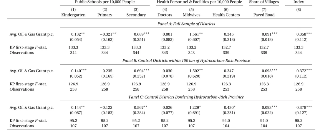
The outcome variables belong to the following categories: public schools, health facilities, health personnel, and road quality. I focus on these outcomes due to data availability and the fact that district governments are responsible for either provision (education and health) or financing (local roads) of these services.28 Panel B of Table1provides summary statistics. All
28Village governments play a lead role in the upgrading and maintenance of local infrastructure, such as roads,
bridges, and piped water systems. Districts contribute to the financing of village infrastructure projects and procure engineers, but in most cases village governments initiate and implement the projects (World Bank, 2010).
of the measures of public service delivery involve either lumpy investment (schools, health clinics, road quality) or committed expenditure (health personnel). The theory predicts that the general grant will have a larger impact on these outcomes than the oil and gas grant, and that the outcomes may not even respond to the oil and gas grant.
5.2 Identifying Assumptions
As previously discussed, the key identifying assumption is that districts with different exposure to the grant shocks would have experienced similar trends in public service delivery in the absence of shocks to the grants. Apart from the concerns discussed in the context of fiscal responses, one potential problem is that less developed areas could be experiencing catch-up growth in public services over this period. If public service delivery trends differed for districts with different population densities for reasons other than the general grant reform, the estimates would be biased. Catch-up growth in public services would likely produce differential trends prior to the reform, however. I test for differential pretrends ahead.
5.3 Reduced-Form Effects
I begin by estimating the reduced-form impacts of exposure to the two grants on public service delivery using the regression
Yd,t = X ℓ∈L θℓAd·Nd·Dℓt + X ℓ∈L γℓEd·Dℓt +π ′ Xd,t+αd+λi(d),t+ud,t, (8)
whereYd,tis a public service outcome in districtdin survey yeart, andDℓt is an indicator that equals one ift=ℓ. The setL includes all available survey years except for the reference year, 2005. Thusθℓandγℓmeasure the change in the gradients ofY in exposure to the general grant reform and exposure to the oil and gas grant, respectively, between 2005 and yearℓ.
Figure4displays point estimates and 95-percent confidence intervals for the parameters in Equation (8). Panel (a) plots the estimates of {θℓ}. This gradient is roughly constant over time prior to 2006, which means that pretrends were similar for districts with different exposure to the general grant reform.29For almost all outcomes, the gradient increases after 2006, suggesting that the permanent increase in the general grant increased public service delivery. The only exception is public primary schools per capita, for which the gradient decreases after 2006. This decrease is smaller than the increase in the gradient of public secondary schools per capita. As shown in Appendix FigureA.4, the gradient of school access, measured as the share of villages with at least one school, did not change for public primary schools, whereas it increased for public kindergartens and public secondary schools. This suggests that the decrease in the gradient of public primary schools is due to a reduction
29There is a slight upward pretrend in the gradient of public secondary schools, but this pretrend is small