Research Series No. 59
Aid Allocation Effects on Growth and Poverty
A CGE Framework
Evarist Twimukye, Winnie Nabiddo and John Mary Matovu
May 2009
Economic Policy Research Centre (EPRC)
51 Pool Road Makerere University Campus, P. O. Box 7841 Kampala, Uganda Tel: 256-41-541023, Fax: 256-41-541022, Email: [email protected]
Aid Allocation Effects on Growth and Poverty
Evarist Twimukye, Winnie Nabiddo and John Mary Matovu
i
Abstract
It has been argued that increased aid causes Dutch disease as a result of appreciation of the exchange rate which reduces the competitiveness of the country’s exports. In this paper, we argue that if the aid is used productively, there are both short and long-term gains. Applying a recursive dynamic general equilibrium model on Uganda, we find that while the currency appreciates and some exports decline, the overall impact on growth outweighs the losses in competitiveness. In addition, if aid is used productively, poverty would be substantially reduced as long as the aid increase is sustained.
1
A. Introduction:
Significant increase in aid could lead to an appreciation of the shilling and reduction in exports. With a reduction in exports, this could lead to lower growth both in the short and long-term and probably hurt producers involved in the tradable sectors. Most countries have benefited from increased trade and therefore if aid results into appreciation this could suggest that there is an opportunity cost to these increased inflows. For the case of Uganda, about 30 percent of the budget is financed by aid (Uganda Budget, 2008/2009). The question is whether there is any evidence that this aid has had any impact on the competitiveness of Uganda’s exports.
There are several previous studies that have attempted to address this question. In the paper by Adam and Bevan (2003), they find that if aid is spent on public infrastructure, this would generate a productivity bias in favor of non-tradable production. This delivers the largest aggregate return to aid, with the real exchange rate appreciation reduced or reversed and enhanced export performance, but it does so at the cost of deterioration in the income distribution. They also find that income gains accrue predominantly to urban skilled and unskilled households, leaving the rural poor relatively worse off. They also find that the rural poor may also be worse off in absolute terms.
The limitations of this study lies in the level of aggregation of the CGE model used. It only focused on the use of aid for infrastructure development. We extend the methodology to a more disaggregated model by broadening the various uses of aid. We find that depending on what this aid is used for, the rural poor could indeed be beneficiaries of increased aid too. We experiment with various scenarios. First, we assume that the increased aid is not used for any productive activity and thereby increasing the demand for non-tradables. In the second scenario, we assume that all the aid is spent on enhancing the infrastructure development like roads. In the third simulation, we focus on the possibility of using aid for agricultural production enhancement. This could include provision of
2
extension services and production technologies that could increase agricultural yields. Lastly, we run a simulation where aid is mainly invested in the human development of the population. In this case we focus on using the increased aid on spending on education and health.
The results suggest that there would indeed be winners and losers under these various scenarios. As expected, increased aid would lead to significant appreciation of the currency. Also, as the theory predicts, we find that the demand for non-tradables (mainly the services sector) increases. This is also accompanied by a reduction in the level of exports and a switch to imported goods. However, for simulations where aid is used for productive activities, we find that the losses in competitiveness would be compensated for by growth in other sectors. For instance, by directly investing in agriculture where the bulk of the population is employed, this leads to significant productivity gains in the sector resulting into significant poverty reduction for the rural poor. Likewise, by using aid to boost spending on education and health, this increases the labor productivity of both the urban and rural population leading to both short and long-term growth. However, investment in infrastructure could reinforce the Dutch disease effects since it mainly leads to higher demand for non-tradables.1
The rest of the paper is organized as follows. First, we motivate the paper by looking at the recent developments of aid and the movements of the exchange rate and exports. Second, we provide a brief overview of the literature. The third section briefly describes the dataset and model used. Section four presents the results. The last section concludes and provides policy implications.
1
This is without taking into account that other sectors especially the tradable sector benefit indirectly if for example roads are renovated.
3
B. Background and Motivation of the study
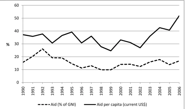
Uganda has received significant amounts of aid since the 1990s, as the county embarked on reconstruction and restructuring under the auspices of the Brentwood institutions. Although aid as a percentage of GNI has not increased much between 1990 and 2006, per capita aid has on the other hand increased significantly from 31 to 51 US dollars in the same period (Fig.1). Because prior to 1995, most of the aid was in form of loans, the country became seriously indebted, a situation that was threatening to derail the growth agenda. By 1992 the country’s external debt stock as a percentage of GDP stood at 97 per cent. In response to the indebtedness of not only Uganda but also most of the developing countries, the UN together with debt cancellation advocate NGOs started a campaign to have these debts cancelled. This led to the so-called Highly Indebted Poor Countries (HIPC) initiative that resulted in the cancellation of the debt owed to multinational and most of the bilateral donors. As a result of HIPC, Uganda received total debt relief and the country’s debt to GDP ratio had reduced to 58 per cent of GDP by 1999. But consequent to that, Uganda’s debt started to climb again with the Debt to GDP ratio hitting 67 per cent by 2003. The country then received more debt cancellation in 2005 under the Multilateral Debt Relief Initiative (MDRI), and as result of HIPC and this new initiative, Uganda’s external debt had reduced to just 47 per cent of GDP as of 2006 (Fig. 3).
4
Fig. 1: Uganda’s Total Aid (% of GNI) and Aid Per capita (Current US$), 1990-2006
Source: World Development Indicators, 2007
To ensure continued sustainable external debt, the government in 1995 put in place an external debt strategy which was modified further in 2007. Under this strategy, the government decided to give grants priority over loans, and to strictly adhere to concessional terms, limit borrowing to only five priority areas especially in infrastructure, and to set a 5-year borrowing cap. In addition the government decided that debt is aligned with absorptive capacity and availability of government counter-funding. Since the government has a Medium Term Expenditure Frame Work (MTEF), the intention is to make sure that all the borrowing is within the MTEF limits and that there is enough absorption capacity for the resources.
0 10 20 30 40 50 60 1990 1991 1992 1993 1994 1995 1996 1997 1998 1999 2000 2001 2002 2003 2004 2005 2006 %
5
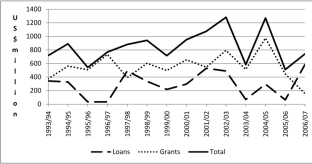
Figure 2: Donor Commitments for Financial Years 1993/94-2006/07
Source: Ministry of Fiance, Planning and Economic Develeopment (MFPED) Consequently, Uganda has been receiving most of the external assistance in form of grants. Indeed, since 1995, grants have persistently been above loan receipts except in 1996/07 and 2006/07 (Fig. 2).The increase in the grant disbursements even as the amount of loans was going down ensured that the total aid has increased over the years. Due partly to persistent high levels of poverty, especially in the rural areas, in spite of the high levels of aid the country has received in the last two decades, but also because of the fear of the country falling again into a serious debt trap, there have been concerns that the aid is not being spent in areas that help to improve the welfare of the population. The concern arises from the fact that increased aid (more so in form of loans, but even in form of grants), if not spent in productive areas of the economy may harm the economy.
0 200 400 600 800 1000 1200 1400 1993/94 1994/95 1995/96 1996/97 1997/98 1998/99 1999/00 2000/01 2001/02 2002/03 2003/04 2004/05 2005/06 2006/07 U S $ m i l l i o n
6
Figure 3: Stock of Total External Debt (percentage of GDP) and Debt Service (percentage of Exports of Goods and Services)
Source: MFPED.
For example in the Financial Year 2000/01, more than 11 per cent of the aid received was spent on public administration (considered to be non-productive spending), a figure that was higher than what was spent on agriculture and education combined -10 percent (Table 1).
One recent feature of the aid expenditure has been the increasing share of aid that is channeled through budget support (from 30 per cent 2000/01 to 50 per cent in 2006/07) as opposed to targeted sectoral support. Though the government prefers this arrangement for better monetary and fiscal planning, the danger is that the aid channeled under budget support may not be easily targeted to productive sectors as donors lose the control of the process. For example, whereas the share of aid spent on public expenditure appears to have gone down (from 11.5 per cent in 2000/01 to 1.9 per cent); it is also true that there has been concurrent increase in budget support (from 30.4 per cent to 50 per cent in the same period). The problem is that as more resources get
96.8 85.4 78.5 61.0 60.0 60.1 55.1 58.1 60.5 60.0 65.1 67.4 65.5 50.6 47.3 1992 1993 1994 1995 1996 1997 1998 1999 2000 2001 2002 2003 2004 2005 2006 %
7
channeled through budget support, priority areas get crowded in other not essential expenditures funded through the budget. For example, though it may appear that security (or defense) does not get funded by aid money, the increase in defense spending in the budget has gone hand in hand with the increase in the share of aid channeled through budget support (Table 1). Consequently, due to the fungibility of money, as more resources through the budget (even if the resources are domestically generated) go to financing non-productive sectors of the economy like public administration and defense, it is inevitable that more aid will indirectly be used for unproductive purposes. Such aid may lead to Dutch Disease and harm the competitiveness of the country’s exports.
Several studies have found a tendency for aid inflows to be associated with an appreciation of the real exchange rate (see Kasekende and Atingi-Ego (1999) for Uganda, as well as cross-country analysis by Adenauer and Vagassky (1998)). However, this evidence is not overwhelmingly significant. Econometric estimates often show the impact of aid on the exchange rate to be small and statistically insignificant. Prati, et.al (2003), suggest that for countries whose official development assistance (ODA) is in excess of 2 percent of GDP a year, a doubling of aid would appreciate the level of real exchange rate by, at most, 4 percent in the short run, rising to about 18 percent over a five-year period, and 30 percent over a decade. Other studies of African countries find that aid inflows appear to be associated with a real depreciation, reflecting increased productivity (supply-side response) as a result of aid (see, for example, Nyoni 1998, Sackey 2001).
Figure 4 suggests that even though Uganda has continued to witness a surge in total aid flows, it is difficult to infer from the figure that the increase in aid was accompanied by the appreciation of the REER. From a casual look, during some periods we observe that indeed when aid increased instead we observe a depreciation of the currency. In other periods, the Dutch disease theory holds. Likewise, when we critically look at the figure for exports, there is no systematic
8
relationship in the decline of exports and increase in foreign aid. This is partly due to that fact that the relationship between foreign aid, exchange rate and the domestic production are more complicated. This therefore calls for the use of a multi-sectoral model that can adequately capture these intricate relationships.
9
Table 1: Summary of Donor Disbursements by Sector Share (%) 2000/01-2006/07
SECTORS 1998/99 1999/00 2000/01 2001/02 2002/03 2003/04 2004/05 2005/06 2006/07
SECURITY 0.0 0.0 0.0 0.0 0.0 0.0 0.0 0.0 0.0
ROADS & WORKS 16.58 14.7 13.4 9.8 6.4 10.8 10.2 5.6 11.8
AGRICULTURE 3.9 5.2 5.8 4.8 6.8 2.8 3.4 4.6 3.4
EDUCATION 7.4 4.1 3.2 3.1 4.5 3.2 3.0 4.6 1.8
HEALTH 14.8 13.4 10.7 8.0 12.2 7.5 10.9 20.2 13.6
WATER& SANITATION 5.9 6.9 7.3 5.3 2.9 2.8 2.8 4.4 3.3
JUSTICE/LAW & ORDER 0.4 0.5 0.4 0.3 0.8 0.4 0.4 0.1 0.2
ACCOUNTABILITY 0.1 0.2 0.1 0.1 2.7 2.4 1.6 5.1 2.8 ECON.FUN/SOC. 7.5 6.6 8.5 7.1 8.0 11.3 8.5 8.1 6.1 PUBLIC 9.7 10.3 11.5 7.1 4.0 2.6 1.9 2.6 1.9 BUDGET SUPPORT 28.2 31.6 30.4 47.1 40.5 46.0 45.6 32.7 50.0 DEBT RELIEF/HIPC 5.6 6.7 8.9 7.4 8.2 5.8 6.3 11.1 5.0 EMERGENCY RELIEF - - - - 3.0 4.4 5.7 0.9 0.0 GRAND TOTAL 100 100 100.0 100.0 100.0 100.0 100.0 100.0 100.0
10
Fig. 4: NEER, REER and Total Aid Inflows (1993-2007)
Source: Bank of Uganda
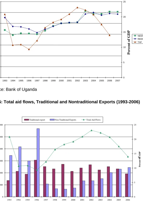
Fig. 5: Total aid flows, Traditional and Nontraditional Exports (1993-2006)
Source: Bank of Uganda 0 100000 200000 300000 400000 500000 600000 1993 1994 1995 1996 1997 1998 1999 2000 2001 2002 2003 2004 2005 2006 Tones 0 5 10 15 20 25 Perc en t of GDP
Traditional export Non Traditional Exports Total Aid Flows
0 20 40 60 80 100 120 140 1993 1994 1995 1996 1997 1998 1999 2000 2001 2002 2003 2004 2005 2006 2007 Index ( 2 00 0= 1 0 0 ) 0 5 10 15 20 25 Percent of GDP NEER REER TAF
11
C. Goals and Objectives of the study
The objective of this study is to investigate whether aid reduces the competitiveness of the traded goods sector. We concentrate on productive sectors that we consider to be tradable and are more likely to be harmed by increased aid inflows- manufacturing and the agriculture, and social services sectors like education and health that may indirectly enhance productivity of the labour force.
We also consider the effect of using aid for various public expenditure programs on the performance of these sectors and on the welfare of the population. The study seeks to find out whether by government allocating resources to the different sectors in the economy may determine the severity of or even prevent Dutch Disease effects.
D. Justification of the study
A number of people have studied the Dutch Disease effects in Uganda (see for example, Adam S. and Bevan L. (2003); Nkusu (2004), Atingi-Ego (2005), World Bank (2007) but none of them have looked in detail at the effect of aid on the different sectors of the economy except Adam S. and Bevan L. (2003), who although they considered this question, their CGE model used a SAM that was very aggregated with only five sectors and three households and two labor categories. Our analysis is based on a more extensive SAM which was recently released by the Uganda National Bureau of Statistics (UBOS), based on 2002 data. It has 49 activities, 49 commodities, 5 household types and 3 labor categories. Basing our analysis on this broader SAM, we will provide better understanding of the effect of aid flows on specific households depending on which activities they are involved in.
This study therefore intends to assess the impact of aid on the sectors of the economy that enhance the competitiveness of the country. The study will go on to consider different scenarios of government expenditure to assess which ones are
12
most beneficial to the enhancement of the competitiveness of the economy and lead to lower poverty levels.
Understanding this will help in the streamlining of government expenditure options so as to target those sectors that not only enhance the competitiveness of the economy but also mitigate the impact of Dutch Disease effects arising from increased aid flows.
E. Literature Review
It is argued that increased aid inflows generate the Dutch disease effect because it leads to the appreciation of the real exchange rate, with a subsequent loss of competitiveness in the tradable sectors as resources are reallocated away from traded towards the non-traded sector, harming exports and consumers switching to more competitive imports.
The effect of aid on the exchange rate, however, depends on how aid is utilized. Literature argues that, as long as aid is channeled into productive sectors of the economy, it will not lead to Dutch disease effects but will instead lead to increased productive capacity that will drive the economy to a higher equilibrium. This makes even more sense when dealing with an undeveloped country like Uganda where the economy operates at under capacity. It is therefore theoretically possible for a country to receive massive amounts of aid but still escape absorption capacity and Dutch disease problems, as long as expenditure of such aid is spent productively.
Nkusu, 2004 observes that during the 2001/02, concerns about a possible aid-induced Dutch disease in Uganda were heightened by widening macroeconomic imbalances and an upward trend in the REER but finds that REER remained stable during the 10 year period between 1991/92 and 200/2001 and non-traditional exports increased remarkably, contrary to the predictions of the Dutch disease model. The paper suggests that the Dutch disease need not materialize in many poor countries that can draw on their idle productive capacity to satisfy the increased
13
demand for non-tradables that large ODA flow induce. Other researchers have also found that fears about the danger of increasing aid may be unfounded if the aid can be invested in productive sectors of the economy. Issa and Ouattara (2004), for example found that well invested aid in Syria increased export competitiveness as opposed to hurting it as the Dutch disease economics suggests.
McKinley, 2005 maintains that Dutch disease effects could be mitigated if ODA was properly spent and absorbed but indicates that many governments either didn’t spend the aid because of fear of inflation or did not absorb it because of the fear of appreciation. DFID, 2002 states that although aid generally leads to appreciation of the nominal and real exchange rates, if recipient governments are flexible in the way they spend the aid by mainly spending it in sectors that enhances productivity, the appreciation will not undermine growth, either in aggregate or in the export sector.
Similarly, Barder (2006) found that it is unlikely that a long term, sustained and predictable increase in aid would through the impact on the real exchange rate, do more harm than good because aid spent in part on improving the supply side-investments in infrastructure, education, government institutions and health results in productivity benefits for the whole economy, which can offset any loss of competitiveness from the Dutch disease effect.
Sackey, 2001 comes to the same findings for Ghana, concluding that aid inflows into Ghana through prudent investment have contrary to standard Dutch disease economics leads to the depreciation of the exchange rate, underpinning the view that if aid is prudently invested by targeting those sectors of the economy that can expand the productivity of the economy, it does not necessary have to lead to Dutch Disease effects.
Gupta, et.al, 2005 advise that governments should aim to implement policies that strengthen the potential impact of aid on growth by essentially making sure that if at all the aid is to be completely absorbed, it should go to those sectors that enhance
14
productivity of the economy lest it leads to appreciation of the exchange rate and hurts competitiveness.
Institutional efficiency in spending the aid is also important as it has a bearing on which sectors of the economy the aid will be spent. It is therefore conceivable that countries with functional institutions are more likely to realize more growth from aid expenditure that those with inefficient bureaucracies. Indeed whereas a study by Clemens, et.al, 2004 found a causal relationship between the short term impact aid and economic growth for Sub Saharan Africa they found that the impact of aid was larger in countries with stronger institutions.
F. The Uganda Social Accounting Matrix (SAM) 2007
A Social Accounting Matrix (SAM) is a table which summarizes the economic activities of all agents in the economy. These agents typically include households, enterprises, government, and the rest of the world (ROW). The relationships included in the SAM include purchase of inputs (goods and services, imports, labour, land, capital etc.); production of commodities; payment of wages, interest rent and taxes; and savings and investment. Like other conventional SAMs, the Uganda SAM is based on a block of production activities, involving factors of production, households, government, stocks and the rest of the world.
The Uganda SAM is a 120 by 120 matrix. The various commodities (domestic production) supplied are purchased and used by households for final consumption (42 per cent of the total), but also a considerable proportion (34 per cent) is demanded and used by producers as intermediate inputs. Only 7 percent of domestic production is exported, while 11 per cent is used for investment and stocks and the remaining 7 percent is used by government for final consumption. Households derive 64 per cent of their income from factor income payments, while the rest accrues from government, inter-household transfers, corporations and the rest of the world. The government earns 32 percent of its income from import tariffs – a relatively high proportion, but a characteristic typical of developing countries. It
15
derives 42 percent of its income from the ROW, which includes international aid and interest. The remainder of government’s income is derived from taxes on products (14 percent), income taxes paid by households (6 percent) and corporate taxes (5 percent).
Investment finance is sourced more or less equally from government (26 per cent), domestic producers (27 per cent) and households (26 per cent), with enterprises providing only 21 per cent. Imports of goods and services account for 87 percent of total expenditure to the ROW. The rest is paid to ROW by domestic household sectors in form of remittances; wage labour from domestic production activity; domestic corporations payments of dividends; income transfers paid by government; and net lending and external debt related payments.
The extent of household dis-aggregation is very important for policy analysis, and involves representative household groups as opposed to individual households. Pyatt and Thorbecke (1976) argue persuasively for a household dis-aggregation that minimizes within-group heterogeneity. This is achieved in the Uganda SAM through the disaggregating of households by rural and urban, and whether households are involved in farming or non farming activities.
The Uganda SAM identifies three labour categories disaggregated by skilled, unskilled and self employed. Land and capital are distributed accordingly to the various household groups.
G. Salient Features of the CGE Model
The CGE model used in the present study is based on a standard CGE model developed by Lofgren, Harris, and Robinson (2002). This is a real model without the financial or banking system (See Table A1). It cannot be used to forecast inflation. The CGE model is calibrated to the 2007 SAM. GAMS software is used to calibrate the model and perform the simulations.
16
Productions and commodities
For all activities, producers maximize profits given their technology and the prices of inputs and output. The production technology is a two-step nested structure. At the bottom level, primary inputs are combined to produce value-added using a CES (constant elasticity of substitution) function. At the top level, aggregated value added is then combined with intermediate input within a fixed coefficient (Leontief) function to give the output. The profit maximization gives the demand for intermediate goods, labour and capital demand. The detailed disaggregation of production activities captures the changing structure of growth due to the pandemic.
The allocation of domestic output between exports and domestic sales is determined using the assumption that domestic producers maximize profits subject to imperfect transformability between these two alternatives. The production possibility frontier of the economy is defined by a constant elasticity of transformation (CET) function between domestic supply and export.
On the demand side, a composite commodity is made up of domestic demand and final imports and it is consumed by households, enterprises, and government. The Armington assumption is used here to distinguish between domestically produced goods and imports. For each good, the model assumes imperfect substitutability (CES function) between imports and the corresponding composite domestic goods. The parameter for CET and CES elasticity used to calibrate the functions used in the CGE model are exogenously determined.
Factor of production
There are 6 primary inputs: 3 labour types, capital, cattle and land. Wages and returns to capital are assumed to adjust so as to clear all the factor markets. Unskilled and self-employed labor is mobile across sectors while capital is assumed to be sector-specific.
17
Institutions
There are three institutions in the model:, households, enterprises and government. Households receive their income from primary factor payments. They also receive transfers from government and the rest of the world. Households pay income taxes and these are proportional to their incomes. Savings and total consumption are assumed to be a fixed proportion of household’s disposable income (income after income taxes). Consumption demand is determined by a Linear Expenditure System (LES) function. Firms receive their income from remuneration of capital; transfers from government and the rest of the world; and net capital transfers from households. Firms pay corporate tax to government and these are proportional to their incomes.
Government revenue is composed of direct taxes collected from households and firms, indirect taxes on domestic activities, domestic value added tax, tariff revenue on imports, factor income to the government, and transfers from the rest of the world. The government also saves and consumes.
Macro closure
Equilibrium in a CGE model is captured by a set of macro closures in a model. Aside from the supply-demand balances in product and factor markets, three macroeconomic balances are specified in the model: (i) fiscal balance, (ii) the external trade balance, and (iii) savings-investment balance. For fiscal balance, government savings is assumed to adjust to equate the different between government revenue and spending. For external balance, foreign savings are fixed with exchange rate adjustment to clear foreign exchange markets. For savings-investment balance, the model assumes that savings are savings-investment driven and adjust through flexible saving rate for firms. Alternative closures, described later, are used in a subset of the model simulations.
Recursive Dynamics
To appropriately capture the dynamic aspects of aid on the economy, this model is extended by building some recursive dynamics by adopting the methodology used in
18
previous studies on Botswana and South Africa (Thurlow, 2007). The dynamics is captured by assuming that investments in the current period are used to build on the new capital stock for the next period. The new capital is allocated across sectors according to the profitability of the various sectors. The labour supply path under different policy scenarios is exogenously provided from a demographic model. The model is initially solved to replicate the SAM of 2007.
H Results
H1. Baseline Scenario
The use of the baseline scenario is to provide a benchmark for the comparison of our simulations. This scenario assumes that business continues as usual with no specific changes made to policy. Foreign aid under the baseline scenario is assumed to grow at a modest rate of 3 percent per annum. We also assume that the government increases its spending by a similar growth rate. We assume that growth in total factor productivity (TFP) for all sectors is about 1 percent and this generates about 6 percent for real GDP growth under the baseline. The government finances its activities from domestic and foreign sources in a manner that is designed to be compatible with macroeconomic stability. The main results of the BASE scenario are summarized in Tables 2.
H2. Increases aid not used for any productive activity
We first run a simulation where the aid inflows increase and they are not being used for any productive activity. The argument has always been that increased aid would lead to increased demand and prices for non-tradables especially services. What this could imply is that jobs in the tradables sector become less attractive and thereby leading to a reduction in growth.
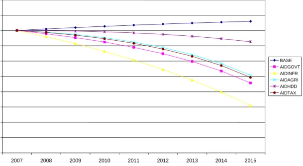
From the results, we find a considerable appreciation of the shilling when we assume that aid is increasing by 5 percent during the years 2008-2015. The effects
19
of this surge in aid flows are consistent with the Dutch-disease theory. Indeed what we find is increased growth in the services sector. Of particular concern is that the growth is mainly in the government services particularly administration. Bevan (2005) notes that the public sector has a higher propensity to consume domestically produced goods and services than the private sector. On the contrary, private services contract over the years. For agriculture, we find significant reduction in production especially for the exportable commodities.
Fig. 6: Exchange Rate Appreciation (2007-2015)
All the traditional exports including cotton, coffee and tea reduce considerably. On the other hand, we also notice a resource shift towards production of non-exportable crops.
There is still considerable uncertainty on the relationship between aid and growth. Some researchers argue that aid could indeed be a disincentive on investments and could indeed be used to finance consumption (Bauer, 1972). Some of the subsequent empirical research did in fact find little or no relation between aid and growth (Mosley, 1980; Singh, 1985). Empirical support for this idea can be found in
0.6 0.65 0.7 0.75 0.8 0.85 0.9 0.95 1 1.05 1.1 2007 2008 2009 2010 2011 2012 2013 2014 2015 BASE AIDGOVT AIDINFR AIDAGRI AIDHDD AIDTAX
20
Boone (1996). A related but distinct strand of the literature examines the impact of aid flows on the tradable goods sector. Most recently, Rajan and Subramanian (2005a) find that aid flows do have adverse effects on growth, wages and unemployment in labor-intensive and export sectors. Other researchers emphasize that the effectiveness of aid depends on the policy environment in the recipient country,Burnside and Dollar (2000).
Overall impact of this scenario on growth is shown in Table 3. On average, due to the loss in competitiveness of the exportable sector, every year the country would lose about 0.4 percent in growth of output. While this is not a lot, cumulatively over the years, it could be significant. Bleaney and Greenway (2001) suggest that an appreciation would hurt investment even though it lowers the price of imported capital goods, because it reduces the returns to investment in the tradables sector. Total export growth on average would grow at 2 percent compared to 8 percent in the baseline scenario.
Fig 7: Overall GDP Growth 2007-2015
The growth for the manufacturing sector is also reduced compared to the baseline where there is no increased aid. Overall, the local manufacturing sector becomes
0 1 2 3 4 5 6 2008 2009 2010 2011 2012 2013 2014 2015 BASE AIDGOVT AIDINFR AIDAGRI AIDHDD AIDTAX
21
less competitive as imports are a lot cheaper. The price rise in non-tradables especially the government sector attracts more resources into the production of non-tradables rather than non-tradables. Since the losses in the tradable sectors are compensated by the increase in the services sector, an argument could be made that increased aid may not be necessarily a bad thing. However, we note from the results that the net impact of aid flows on growth would be negative. In general, government generally employs highly skilled labor. Increased demand for skilled labor which is not abundantly available results into a reduction in production in the manufacturing sector.
INITIAL BASE AIDGOVT AIDINFR AIDAGRI AIDHDD AIDTAX Absorption 26445.5 4.3 4.2 4.8 4.9 5.5 4.7 Consumption 18742.5 4.7 6.0 7.0 6.9 5.6 7.1 Investment 5014.0 4.4 3.2 1.3 1.2 2.2 2.3 Exports 3334.6 8.6 2.1 6.3 2.7 4.2 2.4 Imports 9189.8 4.7 4.6 6.3 5.0 5.5 4.9 Real exchage rate 66.4 -0.5 -2.6 -4.0 -2.0 -1.1 -2.1 Nominal exchange rate 100.0 -0.5 -2.8 -4.2 -2.2 -1.1 -2.3 Investment to GDP 21.8 -0.2 -2.4 -2.6 -2.4 -0.7 -2.7 Foreign Savings to GDP 9.7 -0.4 0.2 0.0 0.2 0.4 0.2 Trade Deficit to GDP 25.5 -0.7 -0.3 -0.6 -0.4 0.0 -0.4 Government Savings GDP 5.3 0.2 -2.7 -2.7 -2.7 -1.2 -2.9
Table 2: Macroeconomic Developments under Various Aid and Spending Scenarios
22
H3. Aid and Increase in Infrastructure Spending
The effects of aid depend on whether it used to improve the productivity of the economy and to remove supply constraints. In this case we focus on a simulation where increased aid is spent on improving infrastructure, particularly roads. The argument is that producers of tradables would then have access to markets and thereby mitigate the losses as a result of the appreciation due to the increased flows.
From the results, we find that with higher spending on infrastructure, the losses due to the appreciation of the currency are reduced. During the years 2008-15, the recovered output would be on average about 0.6 percent of GDP. While exports still remain below the baseline, they are much higher than the case where aid is not productively utilized on infrastructure. The growth path of agriculture and most manufacturing activities does not necessarily improve for a simple reason that increased spending on infrastructure would attract even more resources away from
BASE AIDGOVT AIDINFR AIDAGRI AIDHDD AIDTAX
Overall GDP 4.83 3.74 4.42 4.47 5.27 4.33 Agriculture 3.46 3.71 3.48 6.96 3.46 6.99 Of which Cereals 2.51 1.70 0.74 5.35 2.10 5.30 Root Crops 3.59 4.05 4.40 6.74 3.83 6.76 Pulses 2.57 2.46 2.36 5.91 2.47 5.87 Matooke 3.68 4.45 4.85 6.98 4.05 7.05 Horticulture 3.94 4.94 5.42 7.07 4.40 7.16 Export Crops 2.78 2.42 1.23 6.86 2.61 6.80 Livestock 3.33 3.30 3.32 5.92 3.35 5.95 Forestry 3.69 5.20 5.51 7.18 4.36 7.35 Fishing 4.94 4.40 2.90 9.64 3.94 9.65 Industry 4.78 (1.01) (1.48) (1.15) 3.94 (2.01) Of which Mining 5.00 0.23 (1.88) (0.32) 4.25 (0.98) Manufacturing 4.88 3.08 2.08 3.41 4.38 3.32 Food Processing 4.69 5.06 5.26 5.96 4.67 6.08 Non-Food Processing 5.07 0.76 (2.07) 0.28 4.08 (0.13) Other Industries 4.74 (3.01) (3.10) (3.43) 3.76 (4.79) Services 5.43 5.84 7.23 5.76 6.66 5.78 Private 6.52 5.36 7.29 5.24 5.67 5.26 Public 2.00 7.06 7.09 7.06 9.03 7.09
23
the tradable sectors to the non-tradables.2 However, the growth path of services also remains high being that the large infrastructure projects are provided by the government. Hence the overall increase in demand for non-tradables outweighs the losses incurred due to the un-competitiveness of the export sector. The earlier results by Adams and Bevan (2005) suggests that there may be a case for prioritizing scaled-up infrastructure investment sooner because it will yield a better supply response and offset some of the adverse macroeconomic consequences of scaled-up aid.
The argument could be made that when resources are shifted from tradable commodities to services, this may not be particularly a bad thing. However, a reduction in output for the tradables sectors also creates other economic problems. For the manufacturing sector where labor becomes too expensive due to its excessive demand in the services sector, when production declines that could lead to people losing their jobs and hence an increase in poverty.
The poverty indices shown below suggest that when aid is not used for any productive activity, this results into more people living below the poverty line. The worst affected activities which are agriculture and manufacturing employ more than 80 percent of the population. The bulk of this labor force is mainly in rural areas and tends to be unskilled. As resources get shifted to the non-tradable sector, farming and manufacturing becomes unprofitable and this directly affects the incomes of households involved in the two activities. Indeed, with aid not being productively used, an additional 2 percent of the population would be pushed below the poverty line. However, when the aid is used for productive activities, then the number of household living below the poverty line would be reduced to 18 percent.
The other pertinent question is whether the negative effect on exports is actually of a short-term nature and in the long-run there is a recovery. From the results, it depends on whether the aid flows are sustained over the simulation period. If the aid
2
This is not to make an argument that increased spending on infrastructure is not good for other sectors. Improving the infrastructure has other social benefits beyond the macro-economic implications on other sectors.
24
is sustained over the simulation period, we see a continuous appreciation of the shilling (figure 6). This results into export volumes also declining every period. However, if the aid flow was a one off event, this would result into short-term effects of aid and for the later years exports would recover back to levels higher than the baseline.
Overall, albeit the appreciation of the currency, there are long-term benefit of investments financed by aid – such as in infrastructure in roads—which may improve productivity and growth in both the tradable and non-tradable sector. The overall effect on economic growth of a sustained increase in aid and the corresponding possible contraction in tradables depends on the relative sizes of these two effects.
H4. Aid Targeted to the Agriculture Sector
The previous experiment clearly showed that if aid was utilized to improve infrastructure, this would lead to some gains and mitigate some of the negative effects associated with the Dutch-disease. Since the bulk of the population is employed in the agricultural sector, one would want to know what would happen if most of the aid was used to unleash the binding constraints in this sector. We therefore run a simulation where the aid is used to improve the productivity of the agricultural sector. In this case, aid would be used to provide for example fertilizers, extension services or better technologies that would result into higher yields.
This simulation shows that if aid is appropriately used to enhance productivity in the agricultural sector, this would mitigate the Dutch disease effects associated with the aid flows.
25
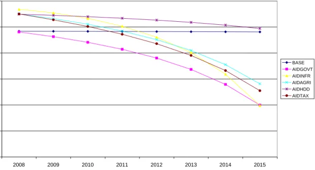
Fig. 8: Agriculture Growth 2007-2015
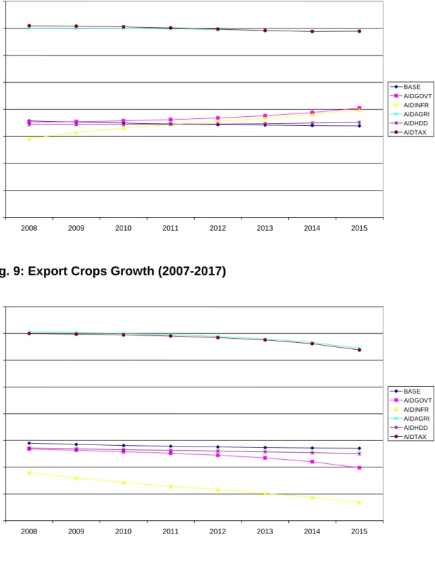
Fig. 9: Export Crops Growth (2007-2017)
0 1 2 3 4 5 6 7 8 2008 2009 2010 2011 2012 2013 2014 2015 BASE AIDGOVT AIDINFR AIDAGRI AIDHDD AIDTAX 0 1 2 3 4 5 6 7 8 2008 2009 2010 2011 2012 2013 2014 2015 BASE AIDGOVT AIDINFR AIDAGRI AIDHDD AIDTAX
26
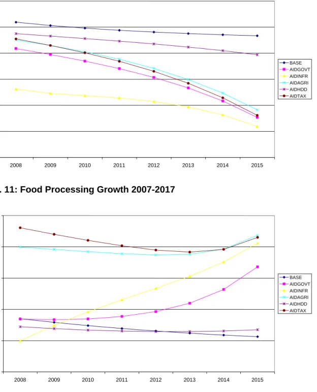
Fig. 10: Manufacturing Growth 2007-2017
Fig. 11: Food Processing Growth 2007-2017
4 4.5 5 5.5 6 6.5 2008 2009 2010 2011 2012 2013 2014 2015 BASE AIDGOVT AIDINFR AIDAGRI AIDHDD AIDTAX 0 1 2 3 4 5 6 2008 2009 2010 2011 2012 2013 2014 2015 BASE AIDGOVT AIDINFR AIDAGRI AIDHDD AIDTAX
27
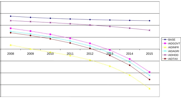
Fig. 12: Non-Food Processing 2007-2017
Fig. 13: Growth in Services (2007-2015)
5 5.5 6 6.5 7 7.5 8 8.5 2008 2009 2010 2011 2012 2013 2014 2015 BASE AIDGOVT AIDINFR AIDAGRI AIDHDD AIDTAX -8 -6 -4 -2 0 2 4 6 8 2008 2009 2010 2011 2012 2013 2014 2015 BASE AIDGOVT AIDINFR AIDAGRI AIDHDD AIDTAX
28
Fig. 14: Private Sector Services Growth (2007-2015)
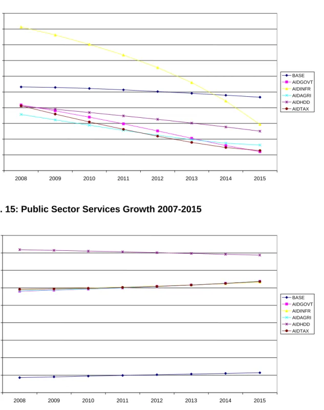
Fig. 15: Public Sector Services Growth 2007-2015
The output recovered if the aid was spent in this sector would be 0.7 percent of GDP on an annual basis. For the exports, we note that they would be a lot higher than the case where aid is not spent productively. Given that a large part of the
1 2 3 4 5 6 7 8 9 10 2008 2009 2010 2011 2012 2013 2014 2015 BASE AIDGOVT AIDINFR AIDAGRI AIDHDD AIDTAX 4 4.5 5 5.5 6 6.5 7 7.5 8 8.5 9 2008 2009 2010 2011 2012 2013 2014 2015 BASE AIDGOVT AIDINFR AIDAGRI AIDHDD AIDTAX
29
manufacturing sector is agro-processing, we also find that manufacturing would not be really as affected given its intermediary link with the more productive agricultural sector. The agro-processing sector would also grow in line with other agricultural activities.
Interestingly, the argument that resources would be shifted to the non-tradables like services would not hold in this case. Indeed, the growth rate of services would be much less than the previous simulation where aid is not used productively.
Given than the majority of the population who are poor are involved in agricultural activities, by targeting the aid resources to the agricultural sector that would also result into the highest reduction in poverty. The welfare of citizens increased through higher levels of consumption – and this is determined not only by what they produce themselves, but also by the additional consumption and investment that the aid finances. What matters for total welfare is the combined effect of a possible reduction in output with the increases in consumption and investment that the aid permits.
H5. Aid and investment in human capital
The alternative use of foreign aid is to invest it in human capital development. In this case the government would put the bulk of the resources in health and education thereby enhancing the skills and productivity of workers. In this context we assume that the increased spending on human capital development would be reflected in the improved service delivery in the health and education sectors. In addition, we tie the productivity of workers to the spending on health and education. Using aid to finance these activities could support the argument that indeed aid enhances the production of non-tradables and could therefore impact negatively on the growth of the country. However, increased social spending in health and education has other indirect benefits particularly the increased productivity of workers. Increased productivity compensates for all the related negative effects of increasing aid. As shown in the figure below we note that overall, growth would be higher by about 0.7 percent if
30
significant aid resources were spent on social areas. While the exportable goods would be hurt under this scenario, the bottom-line remains that the population would be better off albeit the small appreciation.
H6. Aid and Reduction in direct taxes
It can be argued that if there was substantial foreign aid flowing into the country, this could reduce the domestic revenue effort. To an extent, with a reduction in domestic taxes, this could lead to less distortion and could help spur economic growth. On the other hand, this could also lead the country to be aid dependent. In addition, a government that is not getting much revenue from its citizens is not accountable and could also breed corruption (Bevan 2005).
It can also be argued that if the increased aid flow was permanent, rather than improving social services, the government could reward its citizens by reducing direct taxes. In this case, the foreign citizens would be directly financing the consumption of households. This could be an interesting preposition; however it’s difficult to argue for it given the very low tax effort for a country like Uganda. Notwithstanding, the reduction in direct taxes frees up resources available for households, resulting into increased savings and investments for the subsequent periods. The growth rate under this scenario is increased by 0.7 percent compared to the baseline and is also much higher than when the aid is not productively used by the government. We also note the Dutch-disease effects are dominated by the increased resources and production of households even in the tradables sectors particularly exportable crops.
H7. Who are the Winners and Losers
The winners and losers depend so much on the activity a household is involved in. As argued above, it also depends on how the aid is utilized. In a scenario where aid is not productively utilized, the major winners are households involved in the services sector especially the public sector. This is demonstrated in the results
31
where we have a surge in services provided by the public sector. The losers in this case are individuals who are involved in the exportable agricultural commodities. This appreciation of the real exchange rate has a negative impact on rural households producing cash crops for export. By contrast, rural household that produce non-tradable food crops, which are generally the majority, see a rise in incomes. The suppliers of goods and services to government, who tend to live in towns and cities, may gain even more than non-tradable food producers.
Table 4: Poverty Indices under Various Scenarios
However, when the aid is productively used, we find that even households in the tradables sector would benefit from the increased inflows. For instance, households
BASE AIDGOVT AIDINFR AIDAGRI AIDHDD AIDTAX
2007 31.14 31.14 31.14 31.14 31.14 31.14 2008 30.34 30.16 29.80 29.59 29.99 29.47 2009 29.35 29.14 28.25 27.74 28.80 27.55 2010 28.35 28.09 26.32 26.08 27.38 25.89 2011 27.19 26.73 24.92 24.70 26.15 24.31 2012 26.30 25.58 23.21 23.04 25.16 22.57 2013 25.55 24.61 21.49 21.20 23.90 20.92 2014 24.56 23.36 20.22 19.90 22.66 19.71 2015 23.69 22.03 18.90 18.40 21.49 18.31 2007 34.29 34.29 34.29 34.29 34.29 34.29 2008 33.39 33.39 32.99 32.73 33.18 32.60 2009 32.36 32.27 31.28 30.66 31.83 30.46 2010 31.25 31.20 29.29 28.94 30.26 28.78 2011 29.97 29.80 27.91 27.58 28.99 27.17 2012 28.92 28.69 26.12 25.86 28.04 25.35 2013 28.10 27.77 24.26 23.85 26.69 23.56 2014 26.98 26.45 23.00 22.55 25.34 22.37 2015 26.14 25.14 21.62 20.96 24.11 20.88 2007 13.77 13.77 13.77 13.77 13.77 13.77 2008 13.52 12.38 12.26 12.29 12.45 12.26 2009 12.79 11.92 11.54 11.68 12.11 11.48 2010 12.37 10.93 9.98 10.29 11.54 10.00 2011 11.87 9.80 8.44 8.81 10.50 8.53 2012 11.84 8.41 7.16 7.50 9.29 7.22 2013 11.50 7.23 6.25 6.61 8.50 6.38 2014 11.19 6.32 4.92 5.27 7.87 5.06 2015 10.18 4.84 3.87 4.32 7.07 4.12 National Rural Urban
32
involved in the production of traditional exports (including cotton, coffee and tea) would still benefit from the increased aid flows. In addition, if aid is targeted to the development of the human capital of the population, all households whether involved in tradables or non-tradables would benefit. Overall, the incomes of all poor households increase.
I. Conclusions and Policy Implications
Increased aid flows could indeed hurt the economy if not managed well. The Dutch disease effects if aid is spent on unproductive activities are also found to be real. In particular, we find a real exchange rate appreciation that in turn leads to a significant reduction in exports especially the traditional exports. However, if this aid is used on productive activities we find that this could be reversed.
Increased spending on for instance infrastructure leads to higher growth of about 1 percent compared to when the aid is not spent productively. However, this would still be accompanied by a significant reduction in the production of the tradables sector. To mitigate this problem, the government could intervene directly by addressing some of the binding constraints for the tradables sector.
In particular, the tradables sector that is affected most due to the Dutch disease effects of aid inflows are the exportable commodities including the traditional crops and the manufacturing sector. The government could intervene by providing extension services and new technologies to the agricultural sector to enhance the sectors productivity. Likewise, if the government spent a significant proportion of its aid on infrastructure, the productivity of workers would be greatly enhanced and this would result into higher growth both in the short and long-term.
Under all these scenarios, the effects of increased aid flows on poverty depend so much on how the government uses these resources. The households would benefit the most if the bulk of the aid resources were used for the agricultural sector. This is
33
partly because the largest section of the population who are poor are employed in this sector. However, not addressing the Dutch disease effects and their associated effects on exportable commodities could exacerbate poverty especially in the rural areas.
34
References:
Adam S and. Bevan L (2002). “Uganda Aid, Public Expenditure, and Dutch Disease”, Department of Economics, University of Oxford, Working Paper Atingi-Ego (2005). “Budget Support, Aid Dependency, and Dutch Disease: The Case
of Uganda”. Paper presented at the World Bank Practitioners’ Forum, Cape Town
South Africa
Barder, O., (2006). “A policy maker’s guide to Dutch disease”, WP No.91, Center for global Development
Barder, O., (2006) “Are the planned increases in aid too much of a good thing?” WP # 90, Center for Global Development
DFID (2002). “The macroeconomic effect of aid”, A policy paper
Garber, D., S., (2004). “Oil, Dutch disease, and development: the case of Chad”, University of Wisconsin
Issa H & Ouattara, B., (2004). "Foreign Aid Flows and Real Exchange Rate: Evidence from Syria," The School of Economics Discussion Paper Series 0408, Economics, University of Manchester
Lofgren, H., Harris, R. and Robinson, S. 2002. “A Standard Computable General Equilibrium Model in GAMS.” Microcomputers in Policy Research No. 5, International Food Policy Research Institute, Washington, D.C
McKinley, T., (2005). “Why is the ‘Dutch disease’ always a disease? The macroeconomic consequences of scaling up ODA”, IPC, WP No.10
Millennium Project (2004). “Millennium Development Goals Needs Assessments: Country Case Studies of Bangladesh, Cambodia, Ghana, Tanzania and
Uganda”. Working Paper
Nkusu, M. (2004). “Financing Uganda’s Poverty Reduction Strategy: Is Aid Causing More Pain Than Gain?”IMF Working Paper
Sackey, H., A., (2001) “External aid inflows and the real exchange rate in Ghana”, AERC Working Paper 110
Thurlow, J. 2007. Is HIV/AIDS Undermining Botswana’s Success Story? Implications for Development Strategy, IFPRI Discussion Paper 00697
35
Table A1. CGE model sets, parameters, and variables
Symbol Explanation Symbol Explanation
Sets
Activities Commodities not in
CM Activities with a Leontief
function at the top of the technology nest Transaction service commodities Commodities Commodities with domestic production Commodities with domestic sales of domestic output Factors Commodities not in CD Institutions
(domestic and rest of world)
Exported commodities Domestic
institutions Commodities not in CE Domestic non-government institutions ( ) c∈CM ⊂C Aggregate imported commodities Households Parameters Weight of commodity c in the CPI Quantity of stock change Weight of commodity c in the producer price index
Base-year quantity of government demand Quantity of c as
intermediate input per unit of activity a
Base-year quantity of private
investment demand Quantity of commodity c
as trade input per unit of c’ produced and sold domestically
Share for domestic institution i in income of factor f Quantity of commodity c
as trade input per exported unit of c’
Share of net
income of i’ to i (i’ ∈ INSDNG’; i ∈
INSDNG) Quantity of commodity c
as trade input per imported unit of c’
Tax rate for activity a a∈A c∈CMN(⊂C) ( ) a∈ALEO ⊂ A c∈CT(⊂C) c∈C c∈CX(⊂C) ( ) c∈CD ⊂C f ∈F ( ) c∈CDN ⊂C i∈INS ( ) c∈CE ⊂C i∈INSD(⊂INS) ( )
c∈CEN ⊂C i∈INSDNG(⊂INSD)
( ) h∈H ⊂INSDNG c cwts qdstc c dwts qgc ca ica qinvc ' cc icd shifif ' cc ice shiiii' ' cc icm taa
36
Quantity of aggregate intermediate input per activity unit
Exogenous direct tax rate for
domestic institution i
Quantity of aggregate intermediate input per activity unit
0-1 parameter with 1 for institutions with potentially flexed direct tax rates
Base savings rate for
domestic institution i Import tariff rate
0-1 parameter with 1 for institutions with
potentially flexed direct tax rates
Rate of sales tax
Export price (foreign currency)
Transfer from factor f to institution i Import price (foreign
currency) a inta tinsi a iva tins01i i mps tmc i mps01 tqc c pwe trnsfri f c pwm
37
Table A1 continued. CGE model sets, parameters, and variables
Symbol Explanation Symbol Explanation
Greek Symbols
Efficiency parameter in the CES activity function
t cr
δ CET function share
parameter Efficiency parameter in the
CES value-added function
CES value-added function share parameter for factor f in activity a
Shift parameter for domestic commodity aggregation function
Subsistence consumption of marketed commodity c for household h
Armington function shift parameter
Yield of output c per unit of activity a
CET function shift parameter CES production function exponent
a
β Capital sectoral mobility
factor
CES value-added function exponent
Marginal share of
consumption spending on marketed commodity c for household h
Domestic commodity aggregation function exponent
CES activity function share
parameter Armington function exponent
Share parameter for domestic commodity aggregation function
CET function exponent q
cr
δ Armington function share
parameter
a fat
η Sector share of new capital
f
υ Capital depreciation rate
Exogenous Variables
Consumer price index Savings rate scaling factor (=
0 for base) Change in domestic
institution tax share (= 0 for base; exogenous variable)
Quantity supplied of factor
Foreign savings (FCU)
Direct tax scaling factor (= 0 for base; exogenous
variable) Government consumption
adjustment factor
Wage distortion factor for factor f in activity a
Investment adjustment factor Endogenous Variables
a ft
AWF Average capital rental rate in
time period t
Government consumption demand for commodity
Change in domestic Quantity consumed of
a a α va a α va fa δ ac c α m ch γ q c α θac t c α a a ρ va a ρ m ch β ac c ρ a a δ q c ρ ac ac δ t c ρ CPI MPSADJ DTINS QFSf FSAV TINSADJ GADJ WFDISTfa IADJ c QG DMPS QHch
38
institution savings rates (= 0 for base; exogenous
variable)
commodity c by household h
Producer price index for domestically marketed output
Quantity of household home consumption of commodity c from activity a for household h
Government expenditures Quantity of aggregate
intermediate input Consumption spending for
household
Quantity of commodity c as intermediate input to activity a
Exchange rate (LCU per unit of FCU)
Quantity of investment demand for commodity
Government savings QMcr
Quantity of imports of commodity c
Quantity demanded of factor f from activity a
Table A1 continued. CGE model sets, parameters, and variables
Symbol Explanation Symbol Explanation
Endogenous Variables Continued Marginal propensity to save for domestic non-government institution (exogenous variable) Quantity of goods supplied to domestic market (composite supply)
Activity price (unit gross
revenue)
Quantity of commodity demanded as trade input
Demand price for commodity produced and sold domestically
Quantity of (aggregate) value-added
Supply price for commodity produced and sold domestically
Aggregated quantity of domestic output of commodity
cr
PE Export price (domestic
currency)
Quantity of output of commodity c from activity a
Aggregate intermediate
input price for activity a RWFf
Real average factor price
ft
PK Unit price of capital in
time period t
Total nominal absorption cr
PM Import price (domestic
currency)
Direct tax rate for institution i (i ∈ INSDNG)
DPI QHAach
EG QINTAa h EH QINTca EXR QINVc GSAV fa QF i MPS QQc a PA QTc c PDD QVAa c PDS QXc ac QXAC a PINTA TABS i TINS
39
Composite commodity price
Transfers from
institution i’ to i (both in the set INSDNG) Value-added price
(factor income per unit of activity)
Average price of factor Aggregate producer
price for commodity Income of factor f
Producer price of commodity c for activity a Government revenue Quantity (level) of activity Income of domestic non-government institution Quantity sold domestically of domestic output Income to domestic institution i from factor f
cr
QE Quantity of exports ΔKafat
Quantity of new capital by activity a for time period t c PQ TRIIii' a PVA WFf c PX YFf ac PXAC YG a QA YIi c QD YIFif
40
Table A2. CGE model equations Production and Price Equations
c a c a a
QINT =ica ⋅QINTA (1)
a c ca c C PINTA PQ ica ∈ =
∑
⋅ (2)(
)
va va a a 1 -va va vaf a a f a f a f a f F QVA QF ρ ρ α δ α − ∈ ⎛ ⎞ = ⋅⎜ ⋅ ⋅ ⎟ ⎝∑
⎠ (3)(
)
1(
)
1 ' va va a a va vaf va vaf fa f a a f a f a f a f a f a f a f FW WFDIST PVA QVA δ α QF ρ δ α QF ρ
− − − − ∈ ⎛ ⎞ ⋅ = ⋅ ⋅⎜ ⋅ ⋅ ⎟ ⋅ ⋅ ⋅ ⎝
∑
⎠ (4) ' ' ' van van f a f a 1 -van van f a f a f f a f a f F QF QF ρ ρ α δ − ∈ ⎛ ⎞ = ⋅⎜ ⋅ ⎟ ⎝∑
⎠ (5) 1 1 ' ' '' '' ' ' '' van van f a f a van van f f a f f a f a f f a f a f f a f a f F W WFDIST W WFDIST QF δ QF ρ δ QF ρ − − − − ∈ ⎛ ⎞ ⋅ = ⋅ ⋅ ⋅⎜ ⋅ ⎟ ⋅ ⋅ ⎝∑
⎠ (6) a a a QVA =iva QA⋅ (7) a a a QINTA =inta QA⋅ (8) (1 ) a a a a a a aPA ⋅ −ta ⋅QA = PVA QVA⋅ +PINTA QINTA⋅ (9)
a c a c a QXAC =θ ⋅QA (10) a ac ac c C PA PXAC θ ∈ =
∑
⋅ (11) 1 1 ac c ac c ac ac c c a c a c a A QX QXAC ρ ρ α δ − − − ∈ ⎛ ⎞ = ⋅⎜ ⋅ ⎟ ⎝∑
⎠ (12) 1 1 ' ac ac c c ac ac c a c c a c a c a c a c a APXAC = PX QX δ QXAC ρ δ QXAC ρ
− − − − ∈ ⎛ ⎞ ⋅ ⎜⎜ ⋅ ⎟⎟ ⋅ ⋅ ⎝
∑
⎠ (13) ' ' cr cr c c c c CTPE pwe EXR PQ ice
∈ = ⋅ −
∑
⋅ (14) 1 t c t t c c t t t c cr cr c cr c r r = + (1 - ) QX QE QD ρ ρ ρ α ⋅⎛⎜ δ ⋅ δ ⋅ ⎞⎟ ⎝∑
∑
⎠ (15) 1 1 t c t cr cr cr r t c c c 1 - QE PE = QD PDS ρ δ δ − ⎛ ⎞ ⎜ ⋅ ⎟ ⎜ ⎟ ⎜ ⎟ ⎝ ⎠∑
(16)41
Table A3. CGE model equations (continued)
c cr c r = QD QE QX +
∑
(17) c c c c cr cr r PX ⋅QX = PDS QD⋅ +∑
PE ⋅QE (18) ' ' ' c c c c c c CT PDD PDS PQ icd ∈ = +∑
⋅ (19)(
)
' ' ' 1 cr cr cr c c c c CT PM pwm tm EXR PQ icm ∈ = ⋅ + ⋅ +∑
⋅ (20) q q q c c c 1 -- -q q q c cr cr c cr c r r = + (1 - ) QQ α ⋅⎛⎜ δ ⋅QM ρ δ ⋅QD ρ ⎞⎟ ρ ⎝∑
∑
⎠ (21) q c 1 1+ q c cr c q c cr c r QM PDD = 1 - QD PM ρ δ δ ⎛ ⎞ ⎜ ⋅ ⎟ ⎜ ⎟ ⎜ ⎟ ⎝∑
⎠ (22) c c cr r = QQ QD +∑
QM (23)(
1)
c c c c c cr cr r PQ ⋅ −tq ⋅QQ = PDD QD⋅ +∑
PM ⋅QM (24)(
' ' ' ' ' ')
' ' c c c c c c c c c c c C= icm QM ice QE icd
QT QD ∈ ⋅ + ⋅ + ⋅
∑
(25) c c c C CPI PQ cwts ∈ =∑
⋅ (26) c c c C DPI PDS dwts ∈ =∑
⋅ (27)Institutional Incomes and Domestic Demand Equations f a f f f a a A YF = WF WFDIST QF ∈ ⋅ ⋅
∑
(28) i f i f f row fYIF = shif ⋅⎡⎣YF −trnsfr ⋅EXR⎤⎦ (29)
' ' '
i i f i i i gov i row
f F i INSDNG
YI = YIF TRII trnsfr CPI trnsfr EXR
∈ ∈ + + ⋅ + ⋅
∑
∑
(30) ' ' ' ' i ' i i i i i iTRII = shii ⋅(1- MPS ) (1 - tins ) YI⋅ ⋅ (31)
(
)
1 1 h h i h h h i INSDNG EH = shii MPS (1 - tins ) YI ∈ ⎛ ⎞ − ⋅ − ⋅ ⋅ ⎜ ⎟ ⎝∑
⎠ (32) ' ' ' m m m c c h c ch ch h c c h c C PQ QH = PQ γ β EH PQ γ ∈ ⎛ ⎞ ⋅ ⋅ + ⋅⎜ − ⋅ ⎟ ⎝∑
⎠ (33) c cQINV = IADJ qinv⋅ (34)
c c
42
Table A3. CGE Model Equations (continued)
c c i gov
c C i INSDNG
EG PQ QG trnsfr CPI
∈ ∈
=
∑
⋅ +∑
⋅ (36)System Constraints and Macroeconomic Closures
i i c c c c c c
i INSDNG c CMNR c C
gov f gov row
f F YG tins YI tm pwm QM EXR tq PQ QQ YF trnsfr EXR ∈ ∈ ∈ ∈ = ⋅ + ⋅ ⋅ ⋅ + ⋅ ⋅ + + ⋅
∑
∑
∑
∑
(37) c c a c h c c c c a A h H QQ QINT QH QG QINV qdst QT ∈ ∈ =∑
+∑
+ + + + (38) f a f a A QF QFS ∈ =∑
(39) YG=EG GSAV+ (40) cr cr row f cr cr i row r c CMNR f F r c CENR i INSD pwm QM trnsfr pwe QE trnsfr FSAV ∈ ∈ ∈ ∈ ⋅ + = ⋅ + +∑
∑
∑
∑
(41)(
1 i)
i i c c c c i INSDNG c C c CMPS tins YI GSAV EXR FSAV PQ QINV PQ qdst
∈ ∈ ∈ ⋅ − ⋅ + + ⋅ = ⋅ + ⋅
∑
∑
∑
(42)(
1)
i i MPS =mps ⋅ +MPSADJ (43)Capital Accumulation and Allocation Equations
' f a t a f t f t f a t a f a' t a QF AWF WF WFDIST QF ⎡⎛ ⎞ ⎤ ⎢⎜ ⎟ ⎥ = ⎢⎜ ⎟⋅ ⋅ ⎥ ⎜ ⎟ ⎢⎝ ⎠ ⎥ ⎣ ⎦