Biofuels, Policy Options, and Their Implications:
Analyses Using Partial and General Equilibrium
Approaches
Farzad Taheripour and Wallace E. Tyner
Abstract In this chapter, we highlight some important aspects of biofuels devel-opment and policies from partial and general equilibrium perspectives. We first examine US biofuel policy backgrounds to determine factors which caused the boom in the ethanol industry in recent years. Then, we use a partial equilibrium model to investigate the economic consequences of further expansion in the ethanol industry for the key economic variables of the US agricultural and energy mar-kets. This analysis is done for a range of alternative policy options and crude oil prices. Finally, we extend our analyses to examine consequences of further biofuel production at a global scale.
This chapter shows that biofuels policies such as the blending subsidies and the effective ban on use of MTBE have had significant impacts on US biofuel expansion in recent years. In addition, the increased price of crude oil has significantly con-tributed to biofuel expansion. Our analyses indicate that corn ethanol is economic without a subsidy at crude oil prices more than $60 per barrel (even though subsi-dies persist in the United States), but biosubsi-diesel would not exist even at high crude oil prices without government subsidies. Both ethanol and biodiesel production involve potentially large land use changes that take place all over the world. The model and data used for land use change analysis illustrated here need improvement. However, the preliminary results illustrate the kinds of estimated changes that can be produced from the global analysis.
21.1 Introduction
The biofuel industry has been experiencing a period of extraordinary growth, fueled by a combination of high oil prices, ambitious renewable fuel standards, subsidies,
F. Taheripour (B)
Purdue University, West Lafayette, IN, USA e-mail: [email protected]
This chapter is adapted from the authors’ paper that originally appeared in the Journal of
Agricultural and Food Industrial Organization with the following complete reference: Tyner and
Taheripour (2008).
365 M. Khanna et al. (eds.), Handbook of Bioenergy Economics and Policy,
Natural Resource Management and Policy 33, DOI 10.1007/978-1-4419-0369-3_21,
C
and import protection. This rapid growth has important consequences for the United States and global economies. Research studies have examined expansion of biofu-els from different perspectives. Some papers examined price and welfare impacts of these policies for the United States (Rajagopal et al. 2007; de Gorter and Just 2008; Khanna et al. 2008). Several papers have investigated interactions between energy and agricultural markets (Elobeid et al. 2007; Tokgoz et al. 2007; McPhail and Babcock 2008a, b; Tyner and Taheripour 2008b, c). A group of studies have conducted life-cycle analyses of biofuels (Wang 1999, 2005; Farrell et al. 2006; Argonne 2007). In another line of research on biofuels, several papers have studied global economic and land use implications of biofuel policies (Banse et al. 2007; Birur et al. 2007; Taheripour et al. 2008; and Hertel et al. 2008).
In this chapter, we highlight some important aspects of biofuel and biofuel poli-cies from partial and general equilibrium perspectives. We first examine US biofuel policy backgrounds to determine factors which caused the boom in the ethanol industry in recent years. Then, we use a partial equilibrium model to investigate the economic consequences of further expansion in the ethanol industry for the key economic variables of the US agricultural and energy markets under alternative pol-icy options which might be used to promote ethanol production in the future. Finally, we extend our analyses to examine consequences of further biofuel production at a global scale.
Each of these perspectives provides valuable insight into the functioning and impacts of ethanol policy alternatives, and each approach illustrates quite well the newly emerging integration of energy and agricultural markets. Historically, there
has been almost no link between energy and agricultural commodity prices1(Tyner
and Taheripour, 2008b, c). An extensive production of biofuels from agricultural resources links energy and agricultural markets tightly. This chapter demonstrates how the US ethanol policies affect the integrated agricultural and energy markets from partial and general equilibrium angles.
We develop a partial equilibrium analysis at the firm level to review factors which have contributed to the recent boon in ethanol production. This partial equilibrium analysis is built upon the firm level analysis that has been extensively reported in our previous work (Tyner and Taheripour 2007, 2008a). Unlike our earlier work, here we introduce a new break-even comparison for combinations of corn and ethanol prices, which keep a representative dry milling ethanol plant at the zero profit condition. We use this instrument to examine the profitability of the ethanol industry in 2000–2008. Then, we extend our partial equilibrium analyses to examine the link between agricultural and energy markets. The partial equilibrium analysis at the market level extends our earlier work in this context (Tyner and Taheripour 2008b, c) and exam-ines economic consequences of policies which are designed (or can be used) to
1Several articles have addressed the impacts of higher energy prices on the agricultural costs of production (examples are Dvoskin and Heady 1976; Christensen et al. 1981). These papers do not address the link between these markets on the demand side. Even with energy being an influence on cost of production, there has been very low correlation historically between energy and agricultural commodity prices.
promote ethanol production in the United States. In this chapter, we review impacts of fixed and variable subsidies, mandates, and their combinations.
Finally, we use a general equilibrium framework to examine the global economic and land use implications of international biofuel mandate policies. The global gen-eral equilibrium analysis is built upon Taheripour et al. (2008) and Hertel et al. (2008) and concentrates on the impacts of the US and EU biofuel mandate policies. The chapter indicates that, from each of the perspectives, we have entered a new era in which crude oil prices will have a major impact on corn and other agricul-tural commodity prices, and that the policy alternative we choose will have a major influence on what happens in these markets. At relatively low oil prices, it is the US domestic biofuels policies that dominate, but as oil prices get very high, they become the major driver of the energy–agriculture interactions.
This chapter not only provides useful analysis of different biofuels policy alter-natives, but also highlights the strengths and weaknesses of each analytical approach to the problem. The general equilibrium analysis, for example, is very good at cap-turing economy wide linkages and global impacts but is too aggregated to fully capture what happens in domestic markets and at the firm level. Each of the analyt-ical tools provides useful information in understanding the impacts of US biofuels policy options.
21.2 Policy Background and the Ethanol Boom
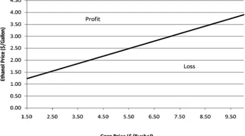
In this section, we first develop a break-even analysis which measures profitability of a representative ethanol producer at all combinations of corn and ethanol prices. Then, we compare the break-even line with the actual observations to examine fac-tors which caused the surge in ethanol industry in recent years. The break-even line
(Fig. 21.1) presents combinations of all corn and ethanol prices,2which keep a new
dry milling ethanol plant at the zero profit condition.3By zero profit, we mean zero
economic profit. The break-even includes a 12% return on equity, so zero profit
means no profit in excess of the 12% equity return.4
Figure 21.1 shows that the representative producer can operate at $2.50 per bushel of corn and $1.55 per gallon of ethanol with no added profit. At relatively higher prices of corn, this combination changes significantly. For example, at $6.50 per bushel of corn the producer must receive $2.80 per gallon of ethanol to operate at the zero profit condition. This indicates that the corn price increases faster than the ethanol price along the break-even line. This is due to the fact that ethanol from corn
2These prices are corn price paid and ethanol price received by the ethanol producer.
3We have modified the Tiffany–Eidman spreadsheet developed at the University of Minnesota (Tiffany and Eidman, 2003) to generate the break-even ethanol and corn prices.
4We also assumed that the price of DDGS is a function of corn and soybean prices. We used historical data to establish the link between these variables. To define a break-even line between corn and crude oil prices, one needs to establish a link between ethanol and crude oil prices. There is no need to establish such a link for the break-even line between corn and ethanol prices.
Fig. 21.1 Break-even ethanol and corn prices
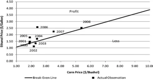
is produced in conjunction with distiller dried grains with solubles (DDGS), which is a valuable feed used in livestock industry. Each bushel of corn can be converted to about 2.79 gallons of denatured ethanol and 18 pounds of DDGS by-product. This product is a good substitute for corn, and its price closely follows the corn price. With this introduction, we now examine factors which caused the boom in the ethanol industry. To facilitate our analysis, we add actual combinations of the corn and ethanol prices to the break-even graph. Figure 21.2 compares the break-even
lines with the actual observations5from the period 2000–2008.
Figure 21.2 reveals that ethanol producers were close to the lower tail of the break-even line at the beginning of 2000s. Given the fact that a portion of the ethanol price received by the producers of this commodity is paid by the federal government
(51 cents prior to 2009 and 45 cents starting in 2009),6 we can conclude that at
the beginning of 2000s the ethanol industry was not profitable without government subsidies. The tax credit helped the industry to operate with low profit margins at the beginning the century.
Subsidization of ethanol in the United States began with the Energy Policy Act of 1978. At the time, the main arguments that were used to justify the subsidy
5Actual observations are annual average prices of corn and ethanol in each year. The 2008 obser-vation represents the average of the first 6 months. The monthly market corn (yellow number 2) prices are obtained from the United States Department of Agriculture website available at:
http://www.ers.usda.gov/data/. The monthly rack ethanol prices are obtained from the Nebraska Government website available at:http://www.neo.ne.gov/statshtml/66.html.
6The ethanol industry share of the blending subsidy is a controversial issue. For a detailed discussion see Taheripour and Tyner (2008).
Fig. 21.2 Break-even corn and ethanol prices compared with actual observations
were enhanced farm income and, to a lesser extent, energy security. In 1990, the Clean Air Act was passed, which required vendors of gasoline to have a mini-mum oxygen percentage in their product. Adding oxygen enables the fuel to burn cleaner, so a cleaner environment became another important justification for ethanol subsidies.
By requiring the oil industry to meet an oxygen percentage standard instead of a direct clean air standard, the policy favored additives like ethanol that contain a high percentage of oxygen by weight. However, methyl tertiary butyl ether (MTBE), a competitor for oxygenation, was generally cheaper than ethanol, so it continued to be the favored way of meeting the oxygen requirements throughout the 1990s. The growth in MTBE use was short lived, as it began to crop up in water supplies in several regions in the country, and it is highly toxic. MTBE was gradually banned on a state-by-state basis.
In 2004, the crude oil price began its steep climb to over $100/bbl. The combi-nation of MTBE ban, low prices of corn, higher crude oil price, and the ethanol tax credit raised profitability of ethanol industry beginning in 2004 and 2005. However, the big increase in ethanol profitability was in 2006 when use of MTBE was effec-tively banned leaving ethanol as the additive of choice. Indeed, ethanol prices peaked at $3.58/gallon in June 2006, shortly after the MTBE ban was complete. Since that time, the price of ethanol has been falling, as the demand for ethanol as an additive has become satiated. In 2007 and the first three quarters of 2008, it appeared that ethanol was increasingly being priced for its energy content – which is only about 70% of that provided by an equivalent volume of gasoline. While in 2006 each gallon of ethanol was making about $1 in profits, the industry moved toward the middle of break-even line in the first 6 months of 2008 with almost no above normal profit. In this time period, the ethanol price has weakly responded to the higher prices of crude oil due to the massive supply of ethanol and its weak
demand. As the result, the profitability of the industry has declined significantly in 2008.
From Fig. 21.2 one can conclude that high profit margins from ethanol produc-tion in 2004–2007 encouraged a rapid investment in ethanol industry in these years. The contribution of the 51 cents per gallon of ethanol subsidy to the profit margin of the industry depends on the distribution of the subsidy among active agents in the corn, ethanol, and gasoline markets.
21.3 Future Ethanol Expansion and Alternative Policy Options
In this section, we extend our analyses to examine impacts of alternative policy options which can be used to promote the ethanol industry on the key economic variables of energy and agricultural markets. We use a partial equilibrium model, which we have developed earlier (Tyner and Taheripour 2008b, c). The partial equilibrium model links agricultural and energy markets and provides a consistent framework to evaluate economic impacts of ethanol supporting policies for the US
economy.7
In this chapter, we design several prospective scenarios which depict the US fuel and corn markets in 2015 for crude oil prices ranging from $40 to $160 per barrel in $20 increments. All of the simulations were done with a 5% fuel demand shock, which basically means that higher income and population by 2015 would stimulate an increase in demand at any given oil price. The simulations also were done with a 40% corn export demand shock to account for the fall of the US dollar. Neither of these shocks was applied to the $40 or $60 oil price cases shown in the figures below, as those cases are included basically for calibration and validation of the model for data in the 2004–2006 period. To focus on impacts of crude price on corn and ethanol markets, we assume no technological improvement in corn production. Of course a major improvement in corn yield could increase corn supply. In design-ing all scenarios, we assume physical constraints such as inadequate infrastructure
and the blending wall8 will not restrict the market. While we recognize that the
blending wall may be a major impediment for further growth in the ethanol indus-try, this analysis abstracts from that issue. The following scenarios are evaluated in this chapter:
7This model assumes that gasoline and ethanol are perfect substitutes and that the price received by ethanol producers is equal to its energy equivalent gasoline price plus the ethanol subsidy, if there is any.
8The blending wall refers to the physical limit on ethanol use with a 10% blend known as E10. We consume about 140 billion gallons of gasoline annually, so 10% would be 14 billion gallons. Due to lack of blending facilities, inability to blend ethanol in southern warm weather states in summer due to its high evaporative emissions, and other infrastructure issues, the effective limit is more like 12–12.5 billion gallons (Tyner et al. 2008). In addition, most vehicles are not flex-fuel and hence they cannot use gasoline blended with ethanol at a rate higher than 10%.
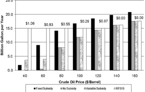
• A fixed ethanol subsidy of 45 cents per gallon, which took effect in January 2009
• No ethanol subsidy
• A variable ethanol subsidy beginning at $70 crude oil and increasing $0.0175 for
each $ crude oil falls below $70
• A renewable fuel standard (RFS) of 15 billion gallons per year from corn ethanol
In what follows, we present impacts of alternative scenarios on the key economic variables of the fuel and corn markets.
21.3.1 Ethanol Production
The simulation results for ethanol production are shown in Fig. 21.3. Several impor-tant conclusions emerge. First, the second bar for each oil price is no subsidy, and it is clear that there is no ethanol production without subsidy unless oil is $60 or higher. This conforms to our earlier firm level analysis. Second, the level of ethanol production with 45 cents fixed subsidy at $40 oil is only 1.8 billion gallons, yet 2004 production was about 3.4 billion. In our previous work with a 51-cent subsidy, we actually got a level close to 3.4 billion, so at low oil prices results are sensitive to the level of the subsidy. Third, at $40 oil, the amount of ethanol production under the variable subsidy is considerably higher than under the fixed subsidy illustrating the potential of the variable subsidy to provide a safety net for low oil prices. Fourth, at oil prices less than $100, ethanol production is higher under the RFS than with the subsidy. However, at any oil price of $100 or higher, production is higher under the
subsidy policy. This is because the RFS mandate is no longer binding at $120 oil or higher. Fifth, the numbers above the RFS bar represent the implicit ethanol subsidy under the RFS. The binding RFS imposes an implicit tax on gasoline consumption and provides an implicit subsidy for ethanol producers to cover their production costs to satisfy the mandate. Consumers pay the implicit tax at the pump when they buy gasoline blended with ethanol at a price higher than what it would be in the absence of mandate. The implicit tax/subsidy approaches zero when the crude oil price increases. The implicit subsidy at $40 crude oil price is about $1.06 per gal-lon, and it goes to zero at $120 crude oil price. Sixth, at oil prices of $140 or higher, there is no difference between the no subsidy, variable subsidy, and RFS cases. The reason again is that at high oil prices, the RFS is not binding. The market alone produces more than the 15 billion gallon mandate.
Finally, it is important to note that as the crude oil price goes up, the ethanol production goes up at a decreasing rate. This is due to the fact that the opportunity costs of producing ethanol from corn goes up with an increasing rate when the crude oil price goes up. As one can see from Fig. 21.3, ethanol production jumps signif-icantly when the crude oil goes from $40 to $60, but when the crude oil goes up from $140 to $160 the ethanol production goes up moderately. This indicates that market forces put automatically a cap on the ethanol production. The increase in corn price is enough to squeeze out profits, so the corn price increase slows substan-tially ethanol growth. Of course, any technological progress or yield improvement can push up the cap.
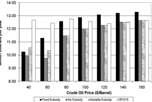
21.3.2 Corn Production
Figure 21.4 displays the amount of corn production for each of the policy options and oil prices. The level of corn production under $40 oil and fixed subsidy, 10.25 billion bushel, is about the actual 2004 value. Corn production must be substantially higher to meet the 15 billion gallon RFS. Again note, that above $120 oil, the RFS is not binding and corn production is market driven. With oil at $100 or higher, the subsidy induces considerably higher corn production. It is important to note that corn production is not only changing due to ethanol production. Corn production responds to other domestic and export demands as well. So corn production could change when the RFS is binding. The small reduction in corn production when no subsidy is available and the price of crude oil increases from $40 to $60 is due to reduction in corn demand for nonethanol uses (food, feed, and exports).
The fraction of corn used for ethanol increases with crude oil price under all alternative policies. For example, with the fixed subsidy in place, only 6.6% of pro-duction of corn is expected to be used in ethanol industry at $40 crude oil price. This figure increases to 57.8% at the $160 crude oil price.
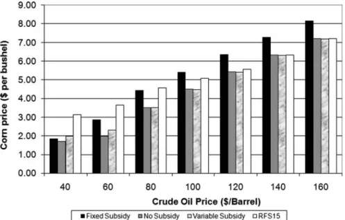
21.3.3 Corn price
Figure 21.5 illustrates the corn price under these same policies and oil prices. At $40 oil, the corn price is a bit under $2 with the 45 cents fixed subsidy policy. In our
Fig. 21.4 Corn production under alternative policy options
previous work with the 51-cent subsidy, the corn price was a bit over $2, which was the case in 2004 with $40 oil. At $140 oil we get a corn price of about $6 under no subsidy, variable subsidy, and RFS. It is about $1 higher with the fixed subsidy. It is striking to see the progression of corn price along with crude oil price. Again, this result illustrates the tight link we will have in the future between crude oil and corn. Of course, in the short run, there will be perturbations due to supply shocks like the 2008 floods and other adjustments, but the long-run relationship should hold.
Figure 21.5 presents the break-even corn–crude oil prices under alternative poli-cies at the market level. One can use this figure to decompose impacts of US ethanol
subsidy and crude oil price on the corn price.9 There is no doubt that ethanol
production in the United States has contributed to higher corn prices. A large por-tion of the growth in corn demand is associated with growth in ethanol producpor-tion. Between 2004 and earlier in 2008, crude oil went from $40 to $120. Over that same time period, corn went from about $2 to about $6. We can partition the $4 corn price increase into two parts: price increase due to the US ethanol subsidy and price increase due to the demand pull of higher crude oil price. Figure 21.5 shows that the corn price under the fixed subsidy is higher than the corn price under the no subsidy case by about $1 for all crude oil prices above $40. Therefore, about $1 of the corn price increase is due to the US subsidy and $3 to the crude oil price increase. The crude oil price increased due to many factors such as higher demand for crude oil,
9This analysis does not consider short-run adjustments in market prices and ignores short-term speculative demand for commodities.
Fig. 21.5 Corn price under alternative policy options
devaluation of the US dollar, political instability in the Middle East, and many other factors. So the crude oil price is the major driver in corn price increase, and the US ethanol subsidy less so. Of course, that was not the case before the surge in crude oil prices. Prior to 2005, the ethanol industry would not have existed without the subsidy.
21.3.4 Corn Exports
Figure 21.6 shows the projected corn exports under alternative policies. Even though we have not yet seen exports fall due to higher corn prices, we would expect to see that after adjustment in global markets. The fall in corn exports shown here is much less that in our previous work, which did not include the 40% export demand shock to account for the falling dollar. Note that in every case, exports are less with the fixed subsidy. Also, as the crude oil price goes up, corn exports decrease as more corn is demanded for ethanol.
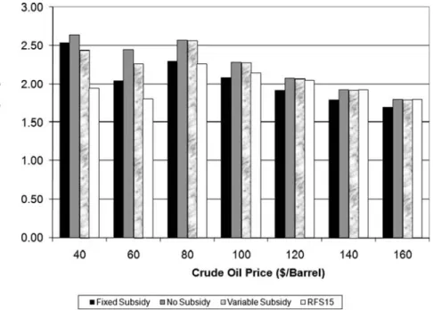
21.3.5 Policy Costs
Figure 21.7 shows the cost of each of the policy instruments for each oil price. Of course, the no subsidy case always has a cost of zero. The RFS cost is paid by the consumer at the pump, whereas the fixed and variable subsidy costs are financed through the government budget. Note that the RFS cost is high at low oil prices and low or zero at high oil prices. The fixed subsidy cost rises linearly with oil price as
Fig. 21.6 Corn exports under alternative policy options
the subsidy supports more ethanol production demanded by the market at higher oil prices. The variable subsidy modeled here has very low costs, and these manifest only at low oil prices. Figure 21.7 indicates that at low crude oil prices, the RFS imposes significant costs on consumers. Alternatively, at oil prices above $80, the cost of the RFS is always lower than the fixed subsidy cost.
21.4 Global Biofuels Impacts
Many countries have announced and implemented plans and programs to increase production and use of biofuels renewable energy. In both the United States and the EU, programs are already in effect that either require or provide incentives for significant production of bioenergy. China, India, Indonesia, and Malaysia, among others, also have announced and implemented biofuels initiatives. More than 13 billion gallons of bioethanol and about 2 billion gallons of biodiesel were produced globally in 2007. This large-scale global implementation of bioenergy production causes global economic, environmental, and social consequences. It can affect the global economy in several ways. In addition, it induces major land use changes across the whole globe, which may lead to significant environmental impacts.
To assess the global impacts of biofuel production, we use a computational general equilibrium (CGE) model which is built upon the standard Global Trade Analysis Project (GTAP) modeling framework (Hertel 1997). GTAP is a CGE model which considers production, consumption, and trade of goods and services by regions and at a global scale. In this model, consumers maximize their utilities according to their budget constraints and producers minimize their production costs subject to resource constraints. The model determines demands for and supplies of goods and services according to consumer and producer behaviors. Resources are labor, capital, land, and natural resources, and they are owned by consumers.
A special version of GTAP, developed by Burniaux and Truong (2002) and modified by McDougall and Golub (2007), incorporates energy into the GTAP framework. Birur et al. (2007) have introduced biofuels into this model. They aug-ment the model by adding the possibility for substitutability between biofuels and petroleum products. Taheripour et al. (2008) have extended the GTAP modeling framework to handle production, consumption, and trade of biofuel by-products. In particular, they introduced distillers dried grains with solubles (DDGS) and oilseed
meals as by-products of ethanol and biodiesel into the model.10 In a recent work
Hertel, Tyner, and Birur (2008) have augmented this model with a land use module to accurately depict the global competition for land among land use sectors. The
10In the extended GTAP model, ethanol and DDGS are jointly produced by the ethanol industry, and biodiesel and oilseed meals are jointly produced by biodiesel industry. So ethanol and DDGS are joint products and biodiesel and oilseed are also joint products. So defining DDGS and oilseed meals as the by-products does not undermine their importance.
land use module disaggregates land into 18 Agro-Ecological Zones (AEZ). These AEZs share common climate, precipitation and moisture conditions, and thereby capture the potential for real competition between alternative land uses. In this chap-ter we use Hertel et al. (2008) and Taheripour et al. (2008) to address two key issues regarding the global impacts of biofuel production. We first highlight the implica-tions of a multinational biofuel mandate for land use change across the world, and then we discuss the importance of incorporating biofuel by-products into the global assessment of biofuel production.
Hertel et al. (2008) have examined the implications of US and EU biofuel
man-date policies for the world economy during the time period of 2006–2015.11 The
United States and EU are major producers of agricultural and livestock commodi-ties. They are also big players in international agricultural markets. Therefore, their biofuel mandate policies are expected to affect agricultural markets and increase competition for land across the world. In addition, their biofuel policies could inter-act and affect direction of changes in resource allocation and land use changes across the world. So it is important to examine consequences of their joint biofuel mandate policies for the global economy. According to Hertel et al. (2008), these mandate policies are expected to affect land use changes across the world and in particular in the United States, EU, and Brazil. To jointly meet the biofuel mandate policies of the United States and EU (ceteris paribus), the cropland areas in the United States, EU, and Brazil would be increased by 0.8, 1.92, and 1.98%, respectively (Table 21.1).
Table 21.1 Percentage change in land cover due to the US–EU biofuel mandate policies (2006– 2015)
Area Cropland Forest Pasture
US 0.8 –3.14 −4.93
EU-27 1.92 −8.34 −9.68
Brazil 1.98 −5.13 −6.3
Note: Figures are percentage changes in productivity adjusted hectares.
We now decompose the impacts of the US and EU policies on cropland. As shown in Table 21.2, about 29% of the change in the cropland areas in the United States occurs due to the EU mandate polices while only about 7% of the change in the EU cropland areas is linked to US mandate policies. Table 21.2 shows that about 27% of changes in the cropland areas of Brazil would be associated with US mandate policies, and the rest would be induced by EU mandate policies. As shown in Table 21.1, the expansion of cropland causes reductions in forest and pasture
11According to these mandate policies, the US corn ethanol production will be equal to 15 billion gallons in 2015. The European Union Biofuels Directive requires that 10% of liquid fuel should be biofuel in the EU region by 2020 (European Commission (2007)). To compare and contrast the EU biofuel directive with the US mandate, it is assumed that the EU will obtain 6.25% of its transportation fuels from biofuels in 2015.
T a ble 21.2 Decomposition o f land co v er impacts o f the US and E U b iofuel mandate policies (%) Cropland F orest P asture Description US–EU mandates Only US mandates Only EU mandates US–EU mandates Only US mandates Only EU mandates US–EU mandates Only US mandates Only EU mandates US 100.0 71.3 28.8 100.0 7 2.9 27.1 100.0 6 8.0 32.0 EU-27 100.0 6 .8 93.2 100.0 6 .5 93.5 100.0 6 .8 93.2 Brazil 100.0 27.3 72.7 100.0 2 9.4 70.6 100.0 2 5.4 74.6
lands. The US and EU mandate policies jointly reduce the forest and pasture land areas of the United States by 3.1 and 4.9%, respectively (Table 21.1). About 73 and 68% of reductions in the US forest and pasture land areas are respectively due to its own biofuel mandate policies, and the rest are due to the EU mandates (Table 21.2). US mandate policies have a small impact on forest and pasture land areas in the EU. While both the US and EU mandate policies induce land use changes in Brazil, the EU mandate policies induce more land use changes in this country compared to the United States (up to 3 times) mainly because the EU needs Brazilian soybeans and soybean oil to meet its biodiesel mandate.
These results clearly indicate that international biofuel policies can interact and induce economic and land use consequences across the world. In other words, con-sequences of producing biofuel in one region can be passed on to other regions as well.
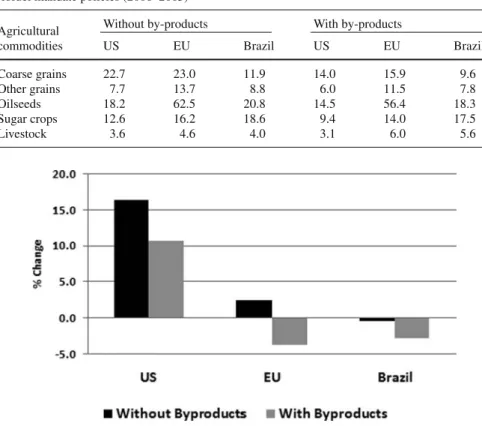
Taheripour et al. (2008) have shown the importance of incorporating biofuel products into the economic analysis of biofuels policies. The model with by-products reveals that production of distillers dried grains with solubles (DDGS) and biodiesel by-products (BDBP) would grow sharply in the United States and EU. For example, the US production of DDGS would grow from 12.5 million metric tons in 2006 to 34 million metric tons if it reaches to its target for ethanol produc-tion in 2015. A major porproduc-tion of this by-product would be used within the United States, and the rest would be exported to other regions such as Canada, EU members, Mexico, China, African and Asian countries. On the other hand, the EU production of BDBP would grow from about 6.1 million metric tons in 2006 to 32.5 million metric tons if it reaches to its target for biodiesel production in 2015. The EU pro-duction of BDBP would be mainly used within this region. The CGE models with and without by-products tell quite different stories regarding the economic impacts of the US and EU biofuel mandates policies. Impacts of these policies on the out-puts and prices of agricultural commodities are shown in Tables 21.3 and 21.4 for the United States, EU, and Brazil.
Table 21.3 Percentage changes in the outputs of agricultural commodities due to the US–EU biofuel mandate policies (2006–2015)
Without by-products With by-products Agricultural
commodities US EU Brazil US EU Brazil
Coarse grains 16.4 2.5 −0.3 10.8 −3.7 −2.8
Other grains −7.5 −12.2 −8.7 −5.0 −12.2 −8.5
Oilseeds 6.8 51.9 21.1 8.6 53.1 19.0
Sugar crops −1.8 −3.7 8.2 −0.9 −3.3 8.4
Livestock −1.2 −1.7 −1.3 −0.7 −2.1 −2.1
While both models demonstrate significant changes in the agricultural production patterns around the world, the model with by-products shows smaller changes in the production of cereal grains and larger changes for oilseeds in the United States and EU, and the reverse for Brazil. For example, as shown in Table 21.3 and Fig. 21.8,
Table 21.4 Percentage changes in the supply prices of agricultural commodities due to the US–EU biofuel mandate policies (2006–2015)
Without by-products With by-products
Agricultural
commodities US EU Brazil US EU Brazil
Coarse grains 22.7 23.0 11.9 14.0 15.9 9.6
Other grains 7.7 13.7 8.8 6.0 11.5 7.8
Oilseeds 18.2 62.5 20.8 14.5 56.4 18.3
Sugar crops 12.6 16.2 18.6 9.4 14.0 17.5
Livestock 3.6 4.6 4.0 3.1 6.0 5.6
Fig. 21.8 Percentage change in coarse grain production due to the US and EU biofuel mandate policies 2006–2015
the US production of cereal grains increases by 10.8 and 16.4% with and without by-products, respectively. The difference between these two numbers corresponds to 646 million bushels of corn, which could be used to produce about 1.7 billion gal-lons of ethanol. This is really a big number to ignore and disregard in the economic analyses of biofuel production.
With by-products included in the model, prices change less due to the mandate policies. For example, as shown in Table 21.4, the model with no by-products pre-dicts that the price of cereal grains grows 23% in the United States during the time period of 2006–2015. The corresponding number for the model with by-products is 14%.
Introducing by-products into the model alters the trade effects of the US–EU mandate policies as well. For example, as shown in Table 21.5, the model with no by-products estimates that the US exports of coarse grains to the EU, Brazil, and Latin American region would be sharply dropped by –4.8, –25.5, and –12.7%, respectively. The corresponding figures for the model with by-products are –2.1, –15.7, and –7.9%.
Table 21.5 Percentage changes in the quantities of US exports of grains and oilseeds to the selected regains due to the US–EU biofuel mandate policies (2006–2015)
Without by-products With by-products
Commodity EU Brazil LAEEXa EU Brazil LAEEXa
Coarse grains −4.8 −25.5 −12.7 −2.1 −15.7 −7.9
Other grains 32.0 −9.3 −8.7 31.4 −4.7 −5.9
Oilseeds 105.7 −4.1 −11.3 109.4 0.4 −8.7
aLAEEX is an abbreviation for Latin American Energy Exporting Countries.
21.5 Conclusions
Clearly, biofuels policies have major impacts on the level of production and the global distribution of impacts. In addition, other factors such as the effective ban on use of MTBE in the United States in 2006 also have had a significant impact. Clearly also the increased price of crude oil has a very important impact on ethanol production. It is important to note that ethanol production both from sugarcane and corn is largely driven by the oil price, whereas biodiesel is driven mainly by gov-ernment policies. That is, ethanol is economic without a subsidy at crude oil prices more than $60 per barrel (even though subsidies persist in the United States), but biodiesel would not exist even at high oil prices without government subsidies. Both ethanol and biodiesel production involve potentially large land use changes that take place all over the world. The model and data used for land use change analysis illus-trated here need improvement. However, the numbers shown here illustrate the kinds of results that can be produced from the global analysis.
References
Argonne National Laboratory (2007) Greenhouse gases, regulated emissions, and energy use in transportation (GREET) computer model. Center for Transportation Research, Energy Systems Division, Argonne National Laboratory, Argonne, IL.
Banse M, van Meijl H, Tabeau A, Woltjer G (2007) Impact of EU Biofuel Policies on World Agricultural and Food Markets. Presented at the 10th Annual Conference on Global Economic Analysis, Purdue University.
Birur D, Hertel T, Tyner W (2007) Impact of Biofuel Production on World Agricultural Markets: A Computable General Equilibrium Analysis. GTAP Working Paper No 53, Center for Global Trade Analysis, Purdue University.
Burniaux J, Truong T (2002) GTAP-E: An Energy-Environmental Version of the GTAP Model. GTAP Technical Paper No. 16, Center for Global Trade Analysis, Purdue University. Christensen DA, Schatzer RJ, Heady EO, English BC (1981) The Effects of Increased
Energy Prices on U.S. Agriculture: An Econometric Approach, Card Report 104 Center for Agricultural and Rural Development, Ames, IA.
de Gorter H, Just DR (2008) “Water” in the U.S. Ethanol Tax Credit and Mandate: Implications for Rectangular Deadweight Costs and the Corn-Oil Price Relationship Review of Agricultural Economics Fall, 30(3), 397–410.
Dvoskin D, Heady EO (1976) U.S. Agricultural Production under Limited Energy Supplies, High Energy Prices, and Expanding Agricultural Exports. Card Report 69 Center for Agricultural and Rural Development, Ames, IA.
Elobeid A, Tokgoz S, Hayes DJ, Babcock BA, Hart CE (2007) The Long-Run Impact of Corn-Based Ethanol on the Grain, Oilseed, and Livestock Sectors with Implications for Biotech Crops. AgBioForum 10(1):11–18.
European Commission (2007) Impact Assessment of the Renewable Energy Roadmap-March 2007, Directorate-General for Agriculture and Rural Development, European Commission, AGRI G-2/WM D.
Farrell AE, Plevin RJ, Turner BT et al. (2006) Ethanol Can Contribute to Energy and Environmental Goals. Science 311, 5760, 506–508.
Hertel T, Tyner W, Birur, D (2008) Biofuels for all? Understanding the Global Impacts of Multinational Mandates. GTAP Working Paper No. 51, Center for Global Trade Analysis, Department of Agricultural Economics, Purdue University.
Hertel T (1997) Global Trade Analysis, Modeling and Applications. Cambridge University Press, Cambridge.
Khanna M, Ando A, Taheripour F (2008) Welfare Effects and Unintended Consequences of Ethanol Subsidies. Review of Agricultural Economics Fall 30(3):411–421.
McDougall R, Golub A (2007) GTAP-E Release 6: A Revised Energy-Environmental Version of the GTAP Model. GTAP Research Memorandum No. 15, Center for Global Trade Analysis, Department of Agricultural Economics, Purdue University.
McPhail LL, Babcock BA (2008a) Short-Run Price and Welfare Impacts of Federal Ethanol Policies. Staff General Research Papers 12943, Iowa State University Department of Economics.
McPhail LL, Babcock BA (2008b) Ethanol, Mandates, and Drought: Insights from a Stochastic Equilibrium Model of the U.S. Corn Market. Staff General Research Papers 12878, Iowa State University, Department of Economics.
Rajagopal D, Sexton SE, Roland-Holst D, Zilberman D (2007) Challenge of Biofuel: Filling the Tank Without Emptying the Stomach? Environmental Research Letters 2:1–9.
Taheripour F, Tyner W (2008) Ethanol Subsidies, Who Gets the Benefits? In Joe Outlaw, James Duffield, and Ernstes (eds), Biofuel, Food & Feed Tradeoffs, Proceeding of a conference held by the Farm Foundation/USDA, at St. Louis, Missouri, April 12–13 2007, Farm Foundation, Pak Brook, IL, 91–98.
Taheripour F, Hertel T, Tyner W, Beckman J, Dileep K (2008) Biofuels and their By-Products: Global Economic and Environmental Implications. Presented at the 11th GTAP Conference, June 12–14 2008, Helsinki, Finland and at the 2008 American Agricultural Economics Association meeting in Orlando Florida.
Tiffany D, Eidman V (2003) Factors Associated with Success of Fuel Ethanol Producers. Staff Paper P03-7. St. Paul, MN: University of Minnesota, Department of Applied Economics.
Tokgoz S, Elobeid A, Fabiosa J, et al. (2007) Emerging Biofuels: Outlook of Effects on U.S. Grain, Oilseed and Livestock Markets. Staff report 07-SR 101 Iowa State University (www.card.iastate.edu)
Tyner W, Taheripour F (2007) Renewable Energy Policy Alternatives for the Future, AJAE, 89(5):1303–1310.
Tyner W, Taheripour F (2008a) Future Biofuels Policy Alternatives, in Joe Outlaw, James Duffield, and Ernstes (eds), Biofuel, Food & Feed Tradeoffs, Proceeding of a conference held by the Farm Foundation/USDA, at St. Louis, Missouri, April 12–13 2007, Farm Foundation, Pak Brook, IL, 2008, 10–18.
Tyner W, Taheripour F (2008b) Policy Options for Integrated Energy and Agricultural Markets. Presented at the Allied Social Science Association meeting in New Orleans, January 2007, and published in the Review of Agricultural Economics, 30(3):387–396
Tyner W, Taheripour F (2008c) Policy Analysis for Integrated Energy and Agricultural Markets in a Partial Equilibrium Framework. Paper Presented at the Transition to a Bio-Economy: Integration of Agricultural and Energy Systems conference on February 12–13, 2008 at the Westin Atlanta Airport planned by the Farm Foundation.
Tyner W, Taheripour F (2008D) Biofuels, Policy Options, and Their Implications: Analyses Using Partial and General Equilibrium Approaches, Journal of Agricultural & Food Industrial Organization, 6(2): Article 9. Available at:http://www.bepress.com/jafio/vol6/iss2/art9
Tyner W, Dooley F, Hurt CS, Quear J (2008) Ethanol Pricing Issues for 2008. Industrial Fuels and Power, February, pp.50–57.
Wang M (2005) Updated Energy and Greenhouse Gas Emission Results of Fuel Ethanol. Presented on the 15th International Symposium on Alcohol Fuels, Sept. 26–28, 2005, San Diego, CA, USA.
Wang M (1999) GREET 1.5 – Transportation Fuel-Cycle Model Volume 1: Methodology, Development, Use, and Results. Center for Transportation Research, Energy Systems Division, Argonne National Laboratory, Argonne, Illinois.