Systematic Equity-Based Credit Risk: A CEV
Model with Jump to Default
∗
Luciano Campi
CEREMADE, Universit´
e Paris Dauphine,
Place du Mar´
echal de Lattre de Tassigny, 75775, Paris Cedex 16, France
Alessandro Sbuelz
†Department of Economics and SAFE Center, University of Verona,
Via Giardino Giusti, 2, 37129, Verona, Italy
Simon Polbennikov
Lehman Brothers International, Europe - Quantitative Fixed Income Research,
25 Bank Street, 30th Floor, London E14 5LE, United Kingdom
Forthcoming in the Journal of Economic Dynamics and Control
Abstract
We use equity as the traded primitive for a detailed analysis of systematic default risk. Default is parsimoniously represented by equity value hitting the zero barrier so that, unlike in reduced-form models, the explicit linkage to thefirm’s capital structure is preserved, but, unlike in structural models, restrictive assumptions on the structure are avoided. Default risk is either jump-like or diffusive. The equity price can jump to default: In line with recent empirical evidence on the jump-to-default risk price, we highlight how reasonable choices of the pricing kernel can imply remarkable differences in the equity-price-dependent status between the objective default intensity and the risk-neutral intensity. As equity returns experience negative diffusive shocks, their CEV-type local variance increases and boosts the objective and risk-neutral probabilities of diffusive default. A parsimonious version of our general model simultaneously enables analytical credit-risk management and analytical pricing of credit-sensitive instruments. Easy cross-asset hedging ensues.
JEL-Classification: G12, G33.
Keywords: Market Price of Credit Risk, Constant-Elasticity-of-Variance (CEV) Diff u-sive Risk, Jump-to-Default Risk, Equity, Corporate Bonds, Credit Default Swaps.
∗This article had previuosly appeared under the title ’Assessing Credit with Equity: A CEV Model with Jump
to Default’, CentER Discussion Paper No. 2005-27, available at at SSRN: http://ssrn.com/abstract=675061.
†Corresponding author: Tel.: +39 045 8054922; fax: +39 045 8054935. E-mail address:
1
Introduction
For individual firms in segments of the market with high default risk, default risk and equity returns exhibit a clear link and default risk appears to be systematic (see Vassalou and Xing (2004)). Estimated market prices of risk do include the jump-to-default risk price, which tends to balloon at times of bear equity markets (see Berndt, Douglas, Duffie, Ferguson, and Schranz (2005) and Berndt, Lookman, and Obreja (2006)). The credit-equity link has been attracting attention from credit risk managers. In their effort of assessing actual distances from default, they have been courting credit-risk models that focus on equity data1 and that, given the systematic nature of default risk, explicitly treat the relationship between the objective prob-ability measure and the pricing measure(s). An equity-based model that directly studies the change of measure related to the prevailing pricing kernel enables a better informed assessment of the objective probability of default by supporting a consistent integration of equity market data, of equity options market data, and of market data on other credit-sensitive instruments. Since cross-asset trading of credit risk has been gaining momentum2 among hedge funds and banks, model by-products like analytical results under the pricing measure(s) will also benefit investors.
Only partial help comes from reduced-form models (see Jarrow and Turnbull (1995) among the seminal papers and the reviews in Lando (2004) and Sch¨onbucher (2003)), as they do not consider the direct linkage to thefirm’s capital structure. Structural models are driven by the value evolution infirm’s assets. The assets-value evolution is often assumed to be diffusive so that the default can be seen predictably coming by observing changes in the capital structure of thefirm (see the seminal papers of Merton (1974) and Black and Cox (1976), and the reviews in Lando (2004) and Sch¨onbucher (2003)). While appealing, structural models suffer when it comes to applications3. The underlying (the sum of firm’s liabilities and equity) is illiquid and often non-tradable. Obtaining accurate asset volatility forecasts and dependable capital structure leverage data is difficult. Predictability of the default event implies the counterfactual prediction of zero credit spreads for short maturities4 and, last but not least, arbitrary use of the structural default barrier is often a temptation hard to resist−endogenous barriers5 come with a practicability issue because the capital-structure assumptions under which they are derived are not fully realistic.
We propose a credit risk model that does look at the firm’s balance sheet but avoids the application mishaps of structural models. We take as underlying the most liquid and observ-able corporate security: Equity6. This modelling choice brings in hedging viability and the
1Fore example, KMV output for publicfirms is strongly driven by equity-value data.
2The rise of capital structure arbitrage is a good example (see Schaefer and Strebulaev (2006)).
3For an empirical analysis of structural models based on corporate-bond price data, see for example Eom,
Helwege, and Huang (2004).
4Zhou (1997) posits assets-value jumps to overcome default predictability. Duffie and Singleton (2001) explain
such jumps with the presence of incomplete accounting information.
5
See for example Leland and Toft (1996), Acharya and Carpenter (2002), and references therein.
6
It must be remarked that, while equity shares are indeed the most liquid and observable securities, equity-based products are not always so. For example, implied volatilities for equity options with strikes such as those
possibility of minimizing the dependability issue in model calibration−leverage information from book values can be circumvented. We represent default as equity value hitting the zero barrier either with a jump or diffusively. The presence of an equity-value drop to zero has its credit-risk foundation in the incompleteness of accounting information (see Duffie and Lando (2001)), rules out default predictability, and embeds the concept of unexpected default, typical of reduced-form models, within a credit-risk model that is directly based on equity. We assume that the continuous-path part of equity value is a Constant-Elasticity-of-Variance (CEV) diffu-sion7, which enables a positive probability8of diffusive absorption at zero. Unlike in structural models, credit risk can be directly related to the so-called ‘leverage effect’ (the negative link between equity returns’ volatility and equity price observed in equity markets as well as in equity options markets) under the CEV assumption, because the primitives are equity returns and their volatility skews rather than the unobserved market value of assets9.
Under these assumptions, we study incomplete-markets equity-based credit risk under the objective probability measure as well as under the pricing measure(s), so that risk premia receive explicit and careful treatment. Our study brings an interesting economic and technical contribution, as the existing literature on equity-based jump-to-default credit risk focuses on pricing-measure analysis10 and avoids the economic and technical treatment of default risk premia. Technically, we prove that the state price densities we consider do back equivalent martingale measures, also in uncharted regions of the parameters where the ‘leverage effect’ is particularly strong. Economically, we show that reasonable choices of the pricing kernel can be consistent with mounting empirical evidence that the two components of the jump-to-default risk price exhibit remarkable differences in their equity-price-dependent status. The jump-to-default risk price is captured by the ratio λQ
λP between the risk-neutral default intensity λQ
and the objective intensity λP. The variance-optimal kernel, which is known to suit market players with hedging needs (for example, see Bertsimas, Kogan, and Lo (2001), Biagini and Cretarola (2005, 2006), Bielecki, Jeanblanc and Rutkowski (2004a, b, c, d), Henderson and Hobson (2003), and Schweizer (2001)), can easily agree with the fact that observed increases in
λQ come from increases in the jump-to-default risk price due to sliding equity valuations rather involved in equity default swaps are not available directly, and often need be mutuated by credit products such as credit default swaps (CDS). There are instances where CDSs provide more liquid information than equity. In general, CDSs are now fundamental liquid credit products.
7
The CEV process has beenfirst introduced tofinance by Cox (1975). Among others, the CEV-based asset-pricing literature includes the works of Albanese, Campolieti, Carr, and Lipton (2001), Beckers (1980), Boyle and Tian (1999), Cox and Ross (1976), Davydov and Linetsky (2001), Emanuel and MacBeth (1982), Forde (2005), Goldenberg (1991), Leung and Kwok (2005), Lo, Hui, Yuen (2000), Lo, Hui, and Yuen (2001), Lo, Tang, Ku, and Hui (2004), Sbuelz (2004), and Schroder (1989).
8Merton (1976) considers equity price’s possible jump to zero, but no diffusive absorption at zero with positive
probability.
9
Hull, Nelken, and White (2004) study the link between credit risk and equity volatility skews in Merton’s (1974) model, within which an option on thefirm’s equity is a compound option on thefirm’s assets.
10
See the pricing analysis in Linetsky (2006), who has introduced some of the pricing motivations for pursuing research on equity-based credit risk, and the pricing analysis in Carr and Linetsky (2006), who have studied the pricing implications of a Jump-to-Default Extended CEV (JDCEV) model.
than from fluctuations in λP. While λP looks pretty stable through time, significant equity-driven variation is observed in the jump-to-default risk price, with recent peaks corresponding to the late-2002 wretched equity markets (see Berndt, Douglas, Duffie, Ferguson, and Schranz (2005) and Berndt, Lookman, and Obreja (2006)). A possible conjecture is that, among other things, keenness to be hedged against default risk might be boosted by bear equity markets, even if they are accompanied by only a slight increase in the objective likelihood of default.
In the second part of this work, we discuss a parsimonious version of our general model. It uses the same technical steps to simultaneously enable analytical credit-risk management and analytical pricing of credit-sensitive instruments. A frugal specification of the state-price density is conducive to a closed form for the objective default probabilities. Under the pricing measure, formulae for Corporate Bond (CB) prices and Credit Default Swap (CDS) fees are obtained, from which hedge ratios can be easily calculated. Empirical tests show that parsimony empowers the model with analytical results without jeopardizing itsflexibility.
Albanese and Chen (2004) and Campi and Sbuelz (2006) also use a CEV-equity model to price credit instruments but they ignore the default predictability issue and the analysis of default-risk premia. In deriving closed-form values, we build upon a CEV result in Campi and Sbuelz (2006). Naik, Trinh, Balakrishnan, and Sen (2003) and Trinh (2004) introduce a hybrid debt-equity model that considers equity as primitive but that, like structural models, necessitates a free default barrier, which is then left to potentially ad-hoc uses−equity value is assumed to be a geometric Brownian motion. Das and Sundaram (2003) have proposed an equity-based model that accounts for default risk, interest risk, and equity risk using a lattice framework. As such, they do not seek hedger-friendly analytical solutions and do not deal explicitly with default-risk premia. Those aspects are also missing in the numerical equity-based credit-risk pricing that has been suggested by the convertible bond11 literature (see, for example, Andersen and Andreasen (2000), Andersen and Buffum (2003), and Tsiveriotis and Fernandes (1998); McConnell and Schwartz (1986) ignore the possibility of bankruptcy). In Cathcart and El-Jahel (2003), default occurs when a geometric-Brownian-motion signaling variable, interpreted as the credit quality of the reference entity, hits a lower default barrier or according to a hazard rate process, so that both expected and unexpected defaults are accomodated in a single framework. However, the signaling variable can hardly be identified with equity value (the default barrier is above the inaccessible zero level and there is no ‘leverage effect’) and the concern of a possibly freewheeling default barrier remains. Such a concern is unlikely to have no impact on the calculation of impied default barriers from market quotes. Hui, Lo, and Tsang (2003) use a dynamic default barrier to achieve an empowered calibration of CB spreads. Brigo and Tarenghi (2005a, 2005b) and Brigo and Morini (2006) employ aflexible time-varying default barrier (the barrier is random in Brigo and Morini (2006)) to accurately calibrate CDS market data.
Linetsky (2006) builds upon the convertible bond literature to assess zero-coupon CB
prices12within a geometric-Brownian-motion model with jump-like bankruptcy where the haz-ard rate of bankruptcy is a negative power of the share price. Carr and Linetsky (2006) consider a general setup of a jump-to-default extended diffusion with arbitrary local volatility and inten-sity functions. In particular, they take the stock price to follow a CEV diffusion, punctuated by a possible jump to zero (the JDCEV model). To capture the possible positive link be-tween default and volatility, they assume that the hazard rate of default is an increasing affine function of the instantaneous variance of returns on the underlying stock. Linetsky (2006) and Carr and Linetsky (2006) pursue a risk-neutral pricing analysis overlooking the study of the existence of some equivalent martingale measure in their incomplete-markets setting−with CEV-like complete markets, Delbaen and Shirakawa (2002) derive existence results for a given lower bound on the CEV parameter. Since default-risk premia are not treated, no discussion of the objective probability of default and of the pricing-kernel-based choice of an equivalent martingale measure is attempted. By contrast, the systematic nature of CEV-like diffusive risk as well as of jump-to-default risk are at the core of our work. In particular, while proving that the pricing kernels13 we study do support equivalent martingale measures, we extend the existence result of Delbaen and Shirakawa (2002) to any negative value of the CEV parame-ter. Such a parameter region is particularly relevant for credit risk: The more negative the CEV parameter, the higher the probability of diffusive default and the more negative the link between equity returns’ volatility and equity price.
The rest of the work is organized as follows. Section 2 describes the general model for the equity market, the market price of credit risk, and its related pricing kernel. Section 3 considers a parsimonious version of the general model that simultaneously enables analytical credit-risk management and analytical pricing of credit-sensitive instruments. Section 4 concludes. An Appendix gathers lengthy proofs, analytical formulae, and details about model extensions with time-dependent coefficients and about model-based hedging.
2
Credit risk under the objective probability measure
A sound assessment of a counterpart’s credit risk under the objective default probability is crucial for any credit risk management system. Financial institutions and banks in particular seek it to assist decisions on approving loans, portfolio monitoring and management reporting,
12
Linetsky (2006) considers recovery payments at maturity. An alternative recovery assumption for corporate bonds is the partial recovery of the face value at the default date regardless of maturity. See later Propositions (5) and (6) and their discussion.
13Since the jump to default is not a stopping time of thefiltration generated by the continuous-path part of
the stock price, our chosen Radon-Nikodym derivative is similar to the one coming from dynamic asset pricing theory with uncertain time-horizon, Blanchet-Scaillet, El Karoui, and Martellini (2005), Proposition 2. Bellamy and Jeanbleanc (2000) analyze the incompleteness of markets driven by a mixed diffusion, construct a similar Radon-Nikodym derivative, and, among other contingent claims, study American contracts. Both Blanchet-Scaillet, El Karoui, and Martellini (2005) and Bellamy and Jeanbleanc (2000) assume bounded local volatility for the stock returns, which is not our CEV case. They also refrain from considering default-driven time-horizon uncertainty.
capital allocation, risk-adjusted performance measurement and loan pricing. Regulatory pres-sure has been adding motivation. The New Basel Capital Accord allows the use of internal ratings systems to determine the appropriate level of reserves to support corporate-exposure activities and other credit risky activities.
We consider an arbitrage-free incomplete market where, under the objective probability measure P, the reference entity’s share price process {S} has the following pre-default jump-diffusion dynamics: dSt St− = µP(St−)dt+σS ρ−1 t− dztP− ³ dNtP−λP(St−)dt ´ , (1)
where{zP} is a Wiener process and {NP} is afirst-jump-stopped marked point process:
NP
t = 1{t≥τ} ,
τ ≡ inf©t:NtP = 1ª (time of the only jump). The underlyingfiltration (Ft) is generated by{zP},{NP}, and
©
ζ1{τ <t} ª
and satisfies the usual conditions of right-continuity andP-completeness. Under (Ft), the jump-risk-pricing random variable ζ (we assume EP[exp(ζ)] bounded) and the processes {zP} and {NP} are mutually independent. While the form ‘σStρ−−1’ of the local diffusive volatility suits the CEV-diffusion focus of the present work, a general form of the local diffusive volatility is fully consistent with the no-arbitrage analysis developed in this section, as long as it is accompanied by a bounded price of diffusive risk and it differs from zero (see later our assumptions on the adapted process
{θ}and see Lemma (1) in the Appendix). By remaining unchanged under the pricing measure of choice, such a general form of the local diffusive volatility agrees with the pricing-measure analysis developed in the sections 2 and 3 of Carr and Linetsky (2006), pp. 306-311. The time of absorption at zero in the absence of jumps isξ, that is
ξ ≡inf{t:St= 0, Nt= 0},
whereas the time of absorption at zerotout court is the minimum betweenτ and ξ, that is
τ∧ξ= inf{t:St= 0}.
The point 0 is the absorbing state of the share-price process {S}, so that, once default has occurred, the share price remains at zero,
The other main objects directly or indirectly appearing in Equation (1) are:
S ≡ S0 (current share price),
St− ≡ limε&0St−ε (left time limit of the share price),
ρ−1 < 0 (constant elasticity of the diffusive volatility),
T > 0 (finite maturity, in years),
λP(St−) ≥ 0 (jump-to-default intensity),
where theP-intensityλP(St−) is a non-negative bounded function of the pre-default share price
St−. The objective chance of seeing no jump is
EtP£1{τ >T}¤=EtP · exp µ − Z T t λP(Su−)du ¶¸ .
We also introduce the time of absorption at zero of the continuous part{Sc}of {S}, that is,
ξc≡inf{t:Stc= 0}, where dStc Stc = µP(St−)dt+σ(S c t)ρ−1dztP+λP(St−)dt. (2)
2.1
Expected equity returns and the market price of credit risk
We take the bounded function θ(St−) as a vehicle of diffusive risk pricing, and the random
variableζ and the positive bounded functionF(St−) as vehicles of jump-to-default risk pricing.
The share’s instantaneous expected capital gain conditional upon St−, µP(St−), takes the following percentage form:
µP(St−) = r−q+θ(St−)σ+
³
EP[exp(ζ)]F(St−)−1
´
λP(St−),
r−q = share’s cost of carry,
θ(St−)σ = premium for the diffusive risk,
¡
EP[exp(ζ)]F(St
−)−1
¢
λP(St−) = premium for the jump-like default risk,
wherer is the constant riskfree rate, q is the constant dividend yield, σ (σ >0) is a constant scale factor for the diffusive volatility.
Proposition (1) states that, in our arbitrage-free incomplete market, the above specification forµP(St−) is equivalent tofix the description of the chosen state-price-density process {π}.
Proposition 1 Fort < τ∧ξ, the P-dynamics of the state-price-density process {π} is dπt πt− = −rdt −θ(St−)St1−−ρ·dzPt +³(exp (ζ)F(St−)−1)·dNtP− ³ EP[exp(ζ)]F(St−)−1 ´ λP(St−)dt ´ , and, fort ≥τ ∧ξ, πt=πτ∧ξexp (−r(t−τ ∧ξ)).
Proof. If the process{π} has the statedP-dynamics (notice that{π}’s expectedP-growth rate is the usual−r as the cumulative premium for the jump-like default risk,
EP[exp(ζ)] Z t
0
(F(Su−)−1)λP(Su−)du,
compensates{π}’s jump process component), then there are no arbitrage opportunities. Indeed, by virtue of Itˆo’s Formula, the π-deflated gain processes generated by holding one share and by holding one unit of currency in the money-market account are localP-martingales,
EtP[d(πt·Stexp (qt))] = 0, EtP[d(πt·exp (rt))] = 0,
and, hence, the market is arbitrage-free14.
As for diffusive risk, the usually-assumed negative relationship between the state-price density and the underlying stock price implies positiveness of the pricing functionθ(St−). If
the premium for diffusive risk vanishes, it is either because such a risk is not priced (supθ↓0) or because the risk is dimming (σ ↓ 0). As for jump risk, the state price density exhibits a sudden move fromπτ− toπτ in the case of a jump to default (τ ∧ξ =τ),
πτ =πτ−exp (ζ)F(St−).
Since πτ represents the fair present value of 1 unit of currency received at the time of
jump-like default per unit probability of such an event, only a structural absence of discontinuity betweenπτ−and πτ will imply that jump-to-default risk is not systematic (exp (ζ)F(St−) = 1 P-a.s.). The element exp (ζ) brings additionalflexibility to the sudden move of the state-price density at the jump-to-default date, on top of the componentF(St−) that relates such a move to the market conditions prevailing just before default. The degree of freedom contributed by exp (ζ) to the {π}-related specification of market participants’ preferences can be valuable in applications.
Given the assumed boundedness of θ(St−) and EP[exp (ζ)]F(St−), the chosen state-price
density process does support an equivalent martingale measureQ. Proposition (2) states that the π-deflated gain process generated by holding one unit of currency in the money-market account is also aP-martingale. Its T-time level represents the Radon-Nikodym derivative ofQ with respect toP,πT exp(rT) = ddQP.
14This rules out arbitrage opportunities involvingStexp (qt) and exp (rt), under natural conditions on dynamic
Proposition 2 Let πt be defined as above and let T >0be any finite time horizon. Then, the localP-martingale process {ertπt}, is a P-martingale over[0, T].
Proof. See the Appendix.
By classic jump-diffusion Cameron-Martin-Girsanov results (see Jacod and Shiryaev (1988)) the risk-neutral jump-to-default intensity λQ(St−) is proportional to the objective intensity
λP(St−) via the pricing kernel’s relative jump at the time of unpredictable default:
λQ(St−)
λP(St−)
=EP[exp (ζ)]F(St−).
Our general shape for the intensities ratio can account for the most recent empiricalfindings on the jump-to-default risk price λQ
λP. Jump-to-default risk is priced ( λQ
λP tends to differ from 1;
cfr. Driessen’s (2005) reduced-form study of corporate debt returns) and its price varies over time with market conditions (λQ
λP varies with St−; cfr. Berndt, Douglas, Duffie, Ferguson, and
Schranz’ (2005) and Saita’s (2006) reduced-form studies of default swap rates and estimated default frequencies and of corporate debt returns, respectively). Interestingly, Berndt, Douglas, Duffie, Ferguson, and Schranz (2005) find that, whileλP tends to have moderatefluctuations over time,λQ is much more time-varying with peaks at times of markets’ reduced risk-bearing capacity (see the situation in the third quarter of 2002). These peaks drive jump-to-defaut risk compensation to relatively high levels. Berndt, Lookman, and Obreja (2006) extend Vassalou and Xing’ (2004) empirical analysis tofind that the interaction between the pricing kernel and equity returns is due mainly to the quantity λQ
λP, which they also find to exhibit considerable
fluctuation through time.
2.2
The
variance-optimal
pricing kernel
In an incomplete market, it is natural to look for a best approximation of a non-attainable claim by the value of a self-financing trading strategy toghether with an initial injection of capital. A quadratic criterion can be used to measure the quality of this approximation, in the sense that the best proxy is taken to be the projection15 of the claim on the value space generated by self-financing strategies. The initial capital associated to the best-proxy strategy can be calculated as the P-expectation of the claim deflated by the variance-optimal pricing kernel process16 {π∗}. Hence, the variance-optimal kernel not only provides the unique no-arbitrage price of attainable claims but also yields the value of non-attainable claims with respect to the reasonable criterion of best quadratic replication. Proposition (3) explicitly carachterizes
{π∗}’s structure in the context of our market.
15
Square integrability is assumed for the claim as well as for the trading strategies’ value. The claim’s terminal date can be the minimum between afixed maturity and a credit-sensitive stopping time. Defaultable-claims hedging has been recently studied by, among others, Biagini and Cretarola (2005, 2006), Bielecki, Jeanblanc and Rutkowski (2004a, b, c, d).
16
Since the pricing kernel {π∗}supports the Radon-Nikodym derivative of the variance-optimal martingale measureQ∗w.r.t. the objective measureP, labelling π∗ ‘variance-optimal kernel’ is a slight abuse of notation thatfinds justification in keeping the credit-risk management analysis under its natural context, that is, under
Proposition 3 Assume the following majorant restriction on the conditional expected excess return on equity:
0≤µP(St−)−(r−q)< σ2St2(−ρ−1)+λP(St−).
The variance-optimal state-price-density process{π∗} is such that
θ∗(St−)St1−−ρ = µP(St−)−(r−q) σ2S2(ρ−1) t− +λP(St−) σStρ−−1, exp (ζ∗)F∗(St−) = 1 + µP(St−)−(r−q) σ2S2(ρ−1) t− +λP(St−) , ζ∗ = 0 P-almost surely.
Proof. In our jump-diffusion setting, the variance-optimal martingale measure coincides
with theminimal martingale measure (the Remark 4.1 in Henderson and Hobson (2003) applies and the majorant restriction on µP(St−) avoids situations in which the minimal martingale
measure is signed), so that{π∗}is also the minimal pricing kernel. The minimal pricing kernel is such thatP-martingales that are orthogonal to the martingale part of the equity price process
{S}remainP-martingales even after being deflated by the minimal kernel itself (cfr. Schweizer (2001) among others). Hence,{π∗} must have the following P-dynamics:
dπ∗ t π∗t− =−rdt+η ∗ t µ dSt St− −µP(St−)dt ¶ , where StdSt
−−µP(St−)dtis the martingale increment of{S}. The kernel{π
∗}must also correctly
price traded securities like equity, that is,
EtP[d(π∗t ·Stexp (qt))] = 0,
or, equivalently by virtue of Itˆo’s Formula,
µP(St−) +q−r+η∗t·σ2S
2(ρ−1)
t− +η∗t ·λP(St−) = 0.
The remark that
θ∗(St−)St1−−ρ=−η∗tσStρ−−1 and exp (ζ∗)F∗(St−)−1 =−η∗t , completes the proof.
The proof emphasizes that{π∗}’s choice is sensible from the point of view of market players with hedging needs. Since {π∗} is also the minimal kernel, the P-expectation of a (possibly non-attainable) claim deflated by {π∗} is not only the initial capital necessary to reproduce the claim’s projection on the value space of self-financing strategies, but also represents the initial cost of the trading strategy that yields an exact replica of the claim and that, although
it may require intermediate injections/withdrawals of cash, is self-financing ‘on average’ and minimizes the conditional size of possible intermediate injections/withdrawals (cfr. Schweizer (2001) among others).
Most importantly, the choice of the pricing kernel {π∗} serves the purpose of highlighting a point of definite interest for credit risk managers: The structure of the pricing kernel at unpredictable default, exp (ζ∗)F∗(St−), implies substantial differences in the ways the objective
default intensity and the risk-neutral intensity depend on equity markets. This is best seen by taking a constant objective intensity λP and a plausibly countercyclical risk premium on equity,
c
µP(St−)−(r−q) =κ·σ2S2(t−ρ−1), 0< κ <1.
From Proposition (3), the variance-optimal pricing kernel hands over a risk-neutral default intensity that is increasing in the diffusive local variance of equity returns:
d λQ∗(St−) = Ã 1 + κ·σ 2S2(ρ−1) t− σ2S2(ρ−1) t− +λP ! λP.
This stylized example17 illustrates the empiricalfinding of Berndt, Douglas, Duffie, Ferguson, and Schranz (2005) that much of time variation in the risk-neutral intensity comes from time variation in the jump-to-default risk price rather than fromfluctuations in the objective inten-sity. Theyfind dramatic equity-market-linked variation over time in the jump-to-default risk price, from peaks in the third quarter of 2002 to a significant drop by late 2003 after the bear market in global equities came to an end in March 2003.
A last remark is in order. The variance-optimal pricing kernel links the market price of diffusive risk with the market price of jump-to-default risk, so that the conditional expected return on equity becomes:
µP(St−)−(r−q) = µ
λQ∗(St−) λP(St−) −
1¶ ³σ2St2(−ρ−1)+λP(St−)´.
Hence, the intensities ratio implied by the variance-optimal pricing kernel can be read in the time-varying betas of a conditional constrained regression of excess stock returns on proxies for the diffusive local variance and for the objective intensity of default (the kernel choice constrains the time-varying betas of the two regressors to be equal).
3
Consistency in risk management and pricing: A
parsimo-nious model
A parsimonious equity-based model that empowers analytical credit risk management as well as analytical pricing of credit-sensitive instruments is valuable. Thrifty formulae for the relevant items underPand underQcan be used to support, among other applications, a consistent and integrated filtering of information from the equity market, equity options markets, and from
17Notice that, sinceλ
Q∗(St−) is not a simple power function in the local variance, the asset-pricing facet of the example is not within the risk-neutral analysis of Carr and Linetsky (2006).
other credit-sensitive markets. Measurement-error issues are trimmed down by model’s explicit focus on the underlying equity value, a clear market signal of corporate health.
Within our general model of Section 2, this is best done by considering the following par-simonious version of it. We take theP-dynamics of the share price process{S}to be
dSt St− = r−q+ θσ+ ¡ EP[exp(ζ)]−1¢λP dt+σStρ−−1dztP− ³ dNtP−λPdt´, (3)
with all the parameters constant. For the sake of simplicity, we assume that unpredictable default is always not liked by investors, that is, the pricing kernel’s ‘percentage jump’ ζ is non-negative. This assumption can be relaxed at zero computational cost, sinceζ can easily be either shifted downwards by adding a negative constant to it or taken with an opposite sign. The criterion of parameter parsimony suggests to take for ζ a one-parameter non-negative distribution. One such distribution is the discrete Poisson distribution with parameterφ(0< φ <∞) and with support{0,1,2, ...}, so that its quantities of interest admit a concise closed form,
EP[exp (ζ)] = exp (φ(e−1))>1, EP[ζ] =V arP[ζ] =φ.
Helpfully, the systematic nature of the jump-to-default risk is turned off(the state-price density does not jump in the case of a jump to default) as the parameter φis turned off(φ↓0, that is, ζ = 0 P-a. s.). An alternative parsimonious choice is the exponential distribution, whose absolute continuity with respect to the Lebesgue measure greatly enrichesζ’s support.
3.1
Default probabilities
Given afinite maturityT (in years),V P(S, T,0) denotes the objective default probability,
VP(S, T, y) ≡ EP0£exp (−y(τ ∧ξ))1{τ∧ξ≤T} ¤
(4)
being the T-truncated Laplace transform of τ ∧ξ’s probability density function under P (P -p.d.f.) with Laplace parameter y (y ≥ 0). The next proposition is a useful result stemming from the independence between{z} and {N}. It states that the quantity in Definition (4) is the linear convex combination of the adjusted objective probability of default withinT (with weight λP
y+λP) and of theT-truncated Laplace transform ofξ c’s
P-p.d.f. with Laplace parameter
y+λP (with weight y+yλ
P).
Proposition 4 The quantity VP(S, T, y) admits the following expression:
VP(S, T, y) = λP y+λP h 1−exp (−(y+λP)T)³1−E0P£1{ξc≤T}¤´i+ y y+λPE P 0 £ exp (−(y+λP)ξc)1{ξc ≤T} ¤ ,
Proof. See the Appendix. TheT-truncated Laplace transform ofξc’sP-p.d.f. with Laplace parameterw≥0,
E0P£exp (−(y+λ)ξc)1{ξc≤T}¤,
is analytical (see Campi and Sbuelz (2006)). Its closed form is also provided in the Appendix.
Equation (3) implies the following Q-dynamics for{S}:
dSt St− = (r−q)dt+σS ρ−1 t− dzQt − ³ dNtQ−λQdt´, (5) ztQ = ztP+ Z t 0
θSu1−−ρdu (Wiener process under Q), λQ = exp (φ(e−1))λP.
When the jump-like default risk is not systematic (φ↓0), the risk-neutral and objective jump-to-default intensities coincide. LetVQ(S, T, y) be theQ-counterpart of the truncated Laplace P-transformVP(S, T, y), that is,
VQ(S, T, y)≡E0Q£exp (−y(τ ∧ξ))1{τ∧ξ≤T} ¤
.
As long as diffusive risk and/or jump-to-default risk are systematic (withζ ≥0), VP(S, T, y) is always smaller than the quantityVQ(S, T, y) for anyy. In particular, systematic risk makes theP-probability of default smaller than theQ-probability of default. The technical reason is that the change of measure fromPtoQleaves diffusive volatility unchanged but, while boosting the jump-to-default intensity (λQ> λP), shrinks the away-from-zero drift of the stock price18:
r−q+λQ < r−q+θσ+λQ=µP+λP.
Thefinancial reason is that the state-price-embedding measureQweighs dislikeable states more than the objective measureP.
3.2
Pricing instruments exposed to credit risk
The quantity
VQ(S, T, y)≡EQ0 £exp (−y(τ ∧ξ))1{τ∧ξ≤T} ¤
is the building block for the analytical pricing of T-year-lived CBs and CDSs. VQ(S, T, r) represents the fair present value of 1 unit of currency at the reference entity’s default if default occurs within T. The next proposition gives an analytical characterization of VQ(S, T, y). An alternative integral expression forVQ(S, T, y) can be found by suitably specializing19 the Formula (5.15) in Carr and Linetsky (2006), p. 320.
18More discussion on this point can be found, among others, in Duffie and Singleton (2003). 19The coefficient ‘c’ in Carr and Linetsky (2006), Equation (4.2), p. 311, must be set to zero.
Proposition 5 TheT-truncated Laplace transform ofτ∧ξ’sQ-p.d.f. with Laplace parameter
y can be expressed as:
VQ(S, T, y) = λQ y+λQ h 1−exp (−(y+λQ)T)³1−E0Q£1{ξc ≤T} ¤´i + y y+λQE Q 0 £ exp (−(y+λQ)ξc)1{ξc ≤T} ¤ .
Proof. Since the risk-neutral drift r−q +λQ is constant, the proof is similar to that of
Proposition (4). The w-discounted value of 1 unit of currency at the diffusive default within
T,
E0Q£exp (−w·ξc)1{ξc
≤T} ¤
,
is analytical20 (see Campi and Sbuelz (2006)).
Proposition (5) engenders analytical pricing of CBs and CDSs. Consider a reference entity’s CB that has face valueF and pays an (annualized) couponC at regular 1k-spaced datesTj up to its maturityT (kis a positive integer). We take the maturityT to be a rational number of the type nk (nis also a positive integer) to keep notation simple.
Proposition 6 Given the recovery rate R at default and given the assumption of Recovery of
Face Value at Default (RFV), the fair CB price is
PCB(S, T, r) = kT X j=1 1 kexp (−rTj) h 1−VQ(S, Tj,0)iC + exp (−rT)h1−VQ(S, T,0)iF +VQ(S, T, r)·R·F.
Proof. The result comes from taking the Q-expectation of CB’s discounted payoffs. RFV
bears the value VQ(S, T, r)·R ·F for CB’s defaultable part as it implies that the relevant discounted payoffis exp (−r(τ∧ξ))1{τ∧ξ≤T}.
Ris a fixed historical data input in applications. Under RFV, CB holders receive the same fractional recovery R of the face value F at default for CBs issued by the reference entity regardless of maturity. Guha and Sbuelz (2005) show that the RFV recovery form is consistent with typical bond indenture language (for example, the claim acceleration clause), defaulted
20Davidov and Linetsky (2001) point out that the quantity EQ
0 £
exp (−wξc)1
{ξc≤T}¤ can be obtained by
numerically inverting the closed-form non-truncated Laplace transform 1 aE Q 0 [exp (−(w+a)ξ c )],
where the inversion parameter isa > 0, see pp. 953 and 956. The same quantity has been also computed in Davydov and Linetsky (2003), Equation (155), p. 206, by means of a spectral expansion (the theory for such an expansion is thoroughly illustrated in Linetsky (2004)). The implementation of Equation (155) requires the numericalfinding of the roots of a Whittaker function (see Equation (90), p. 193) in concert with the calculation of the limit ‘limL↓0’, whereLis a lower price barrier (L < S).
bond price data (same-seniority bonds exhibit the same market value at default regardless of maturity), and relevant stylized facts of non-defaulted bond price data (the low empirical duration of high-yield bonds; see Cornell and Green (1991) and Schaefer and Strebulaev (2006)). Consider a CDS related to the CB just described. It offers a protection payment of (1−R)F
in exchange for an (annualized) feefCDS paid at regular m1-spaced dates up to the contract’s maturity (m is a positive integer).
Proposition 7 The fair CDS fee is
fCDS(S, T, r) = V Q(S, T, r) (1−R) PmT j=1 1 mexp (−rTj) [1−VQ(S, Tj,0)] .
Proof. UnderQ, the feefCDS(S, T, r) makes the CDS’ net present value equal to zero.
The holder of a CB can achieve total recouping of the face value F at default by being long a CDS. Being short ∂S∂ PCB(S, T, r) shares Delta-hedges21 against the pre-default price
shocks driven by diffusive news. Recent empirical evidence shows that hedges based on equity portfolios perform reasonably well for high-yield CBs (see Naik, Trinh, Balakrishnan, and Sen (2003) and Schaefer and Strebulaev (2006)). Given analytical CB prices, an easy and effective measure of the Delta-hedge ratio isPCB’s incremental ratio with respect toS. More details on
model-based CB hedging are in the Appendix.
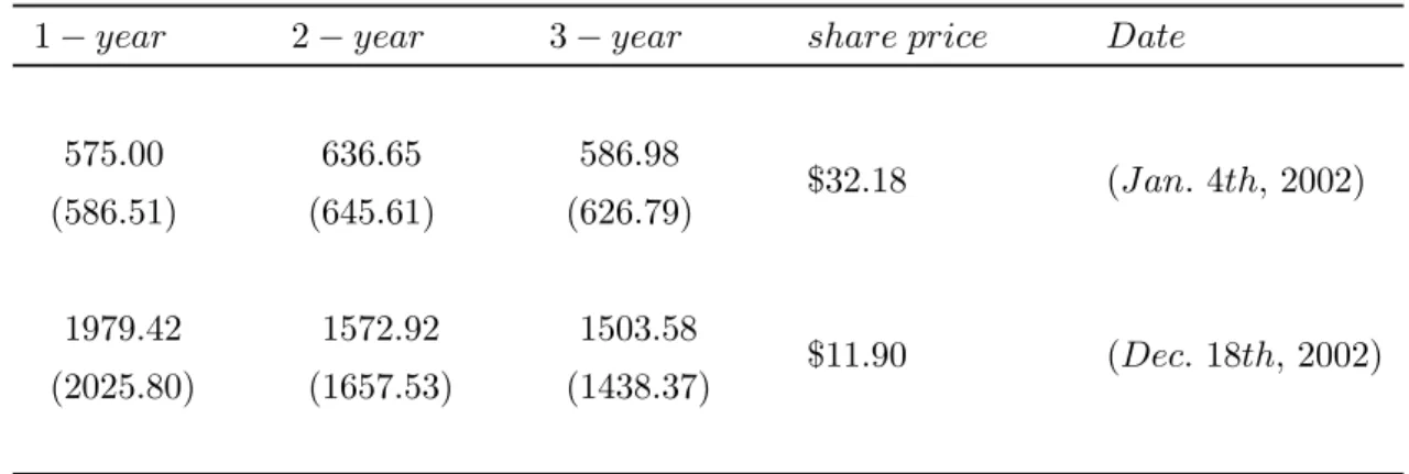
While extensive calibration22 is beyond the scope of the present work, a first interesting empirical test is the troubled market situation, as represented by stock prices and by reliable CDS quotes, of a big American air carrier like Delta Airline in the year 2002. Industry’s long term problems emerged soon after the September 11th, 2001, terrorist attacks and the deep recession in air travel that followed. In addition, America’s top airlines have suffered from huge pension obligations to retired employees andfierce competition from low-cost carriers. As Delta Airline’s stock price dived from about $32 in January 2002 to below $12 by the end of December 2002, the term structure of annualized fees of quarterly CDSs was lifted from levels below 650 basis points to levels above the 1500 basis points and took a downward-sloping shape. Table 1
21
The interest-rate sensitivity of bonds issued by non-high-credit-quality entities is kept quite subdued by the claim acceleration clause. In any case, parallel shifts of the (flat) term structure of the interest rates can be hedged by selling a portfolio of default-free bonds that has interest-rate sensitivity equal to ∂r∂PCB(S, T, r).
Such a hedge ratio can be easily calculated in our model asPCB’s incremental ratio with respect tor.
22
exhibits CDS market quotes23 and, in parentheses, the corresponding model-based quotes. Table 1: CDS fees and share prices, Delta Airline (2002)
1−year 2−year 3−year share price Date
575.00 (586.51) 636.65 (645.61) 586.98 (626.79) $32.18 (Jan.4th, 2002) 1979.42 (2025.80) 1572.92 (1657.53) 1503.58 (1438.37) $11.90 (Dec. 18th,2002)
According to a distance-minimization criterion, the calibration of the model-implied CDS-fee curve to the market curve has been performed by setting the elasticity of the diffusive volatility
ρ−1 equal to−1.1, the recovery rateR equal to 65%, and the risk-neutral intensityλQ equal to 121.5. The parameter σ has been chosen to reproduce the annualized volatility of daily percentage returns on the Delta stock over the last 3 months, which was 58% on January 4th and 115% on December 18th. The other parameters are r = 4.25% (close to the average midpoint of the term structure of US default-free interest rates over the year 2002) andq= 0. Although parsimonious, the model seems flexible in capturing levels and shapes of CDS fees that come along with significative states of equity market valuation.
As CDS markets have been growing by leaps and bounds, reliable quotes can be currently gathered for maturities up to 10 years and the shape of CDS-fee term structures can be confi-dently measured for the 1-to-10-year maturity span. In our last empirical test, the model does show goodness of fit to different patterns of curve steepness. We consider recent Bloomberg data on two American giants of the car industry, which has not been unfamiliar with distress in recent years. For Ford, Table 2 exhibits CDS quotes and, in parentheses, the corresponding model-based quotes.
Table 2: CDS fees and share price, Ford (December 2nd, 2006)
1−year 3−year 5−year 7−year 10−year share price
145.00 (181.41) 405.50 (411.51) 534.75 (536.33) 572.00 (572.84) 584.25 (584.08) $8.04
The calibration of the model-implied CDS-fee curve to the market curve has been implemented byfixing ρ−1 =−0.22, R= 65%, andλQ = 201 . The parameterσ has been chosen to yield a
23
diffusive volatility of 105%. The other parameters arer = 5.25% (about the midpoint of the term structure of US default-free interest rates at the beginning of December 2006) andq= 0. The model is able to match the marked steepness at short maturities andfits well the 5-to-10 year curve. Table 3 exhibits the case of General Motor.
Table 3: CDS fees and share price, General Motor (December 2nd, 2006)
1−year 3−year 5−year 7−year 10−year share price
130.00 (142.55) 296.25 (287.64) 404.92 (406.25) 443.50 (449.53) 463.50 (467.39) $29.85
Calibration has been achieved by takingρ−1 =−0.225,R= 65%, andλQ= 251 . The parameter
σ has been chosen to yield a diffusive volatility of 95%. The other parameters arer = 5.25% and q = 0. The goodness of fit is fine also in this case. In summary, these empirical pricing tests show that thrift has empowered the model with analytical results without jeopardizing itsflexibility.’
4
Conclusions
We present an equity-based credit risk model that, by taking as primitive the most liquid and observable part of afirm’s capital structure, departs from reduced-form models and overcomes many of the problems suffered by structural models in credit-risk management, pricing, and hedging applications. We study systematic credit risk via an explicit modelling of risk premia. This brings an economic and technical contribution to the current literature on equity-based jump-to-default credit risk, which, focused on pricing-measure concerns, has not been dealing with the economic and technical treatment of risk premia and of default risk premia in partic-ular. Technically, we prove that the pricing kernels we study do support equivalent martingale measures, also in unexplored but credit-risk-relevant regions of the parameters. Economically, we show that sensible pricing kernels for hedgers can be consistent with mounting empirical evidence that the jump-to-default risk price heavily loads equity marketfluctuations, reaching highs during bear equity markets. A conceivable conjecture is that bear equity markets might, among other things, exacerbate the propensity to be hedged against default risk even if the increase of such a risk is only marginal. We then discuss a parsimonious version of our gen-eral model that uses the same technical steps to support analytical credit-risk management as well as analytical pricing of credit-sensitive instruments. Empirical tests show that parsimony enriches the model with analytical results without jeopardizing itsflexibility.
As the equity price is becoming a popular measure of the ‘dollar’ distance to default, we believe that future research can capitalize with avail on our model to investigate credit risk
issues that reach over different securities (equity and other credit-sensitive instruments) and over different applications (risk management, pricing, and hedging).
Acknowledgments
We are grateful to the Co-Editor (Carl Chiarella) and to two referees for their detailed feed-back that helped us to refine our manuscript. For many valuable comments and suggestions we wish to thank Rossella Agliardi, Giovanni Barone-Adesi, Anna Battauz, Andrea Berardi, Antje Berndt, Michele Bonollo, Nicole Branger, Andrea Buraschi, Umut Cetin, Francesco Corielli, Rita Laura D’Ecclesia, Marzia De Donno, Darrell Duffie, Andrea Gamba, Martino Grasselli, Rajiv Guha, Monique Jeanblanc, Antonio Mele, Thorsten Rheinlander, Francesco Rossi, Chris-tian Schlag, Claudio Tebaldi, Fabio Trojani, Oldrich Vasicek, Marc Yor, and the participants of the Conference ’From Basel II to Basel III’ Conference (Monte Verit`a - Ascona, March 2006), at the evening sessions of the 2007 CEPR/Studienzentrum Gerzensee European Summer Sym-posia in Financial Markets, at the Annual Conference of the Italian Association of Mathematics Applied to Finance and Economics (Lecce, September 2007), and at the Workshop on Credit Risk Models for Financial Markets and Banking (University of Rimini, October 2007), and the participants at thefinance seminars of the Bocconi University (Milan), the Risk Management Task-Force at the Gruppo Banco Popolare (Verona), and the University ’Tor Vergata’ (Rome).
5
Appendix
Proof of Proposition (2) We will use the following auxiliary result.
Lemma 1 Letρ <1, so possibly taking negative values, letScbe the continuous part ofS with
P-dynamics
dStc Sc
t
= (r−q+θ(Stc)σ+λP(Stc))dt+σ(Stc)ρ−1dzPt,
and letηt be defined as follows:
ηt≡E µ − Z · 0 θ(Stc)(Suc)1−ρdzuP ¶ t , t≥0. (6)
Then, for any 0< T <∞, {η} is a true P-martingale over [0, T]. In particular, E0P[ηT] = 1.
Proof. Following the proof of Theorem 2.3 in Delbaen and Shirakawa (2002), the crucial
argument forηt to be a true P-martingale is that the integral R0Tθ(Stc)2(Suc)2(1−ρ)du is finite a.s.. Delbaen and Shirakawa (2002) show that this is the case forρ ∈(0,1). We notice that this integral remains finite a.s. even forρ≤0. Indeed, since the functionθ(·) is bounded and
Schas continuous trajectories, the integral cannot explode.
To simplify the notation, we seteπt≡ertπt. From Proposition (1) stating{π}’sP-dynamics,
it follows that fort < τ∧ξ
deπt e
πt− =−θ(St−)S
1−ρ
t− dztP+ ((eζF(St−)−1)dNtP−(E0P[eζ]F(St−)−1)λP(St−))dt,
andeπt=eπτ∧ξ fort≥τ∧ξ. The initial condition is of courseeπ0= 1. We can write the process e
πt as a Dol´eans-Dade stochastic exponential (see, e.g., Protter (1990), p. 78) in the following way: e πt=E µ − Z · 0 θ(Su−)Su1−−ρdzPu ¶ t∧τ∧ξ Yt∧τ∧ξ, where we set Yt= exp X u≤t ln(1 + (eζF(Su−)−1)∆NuP)− Z t 0 (E0P[eζ]F(Su−)−1)λP(Su−)du .
Fix afinite time horizonT >0. We first prove that the process
E µ − Z · 0 θ(Su−)Su1−−ρdzuP ¶ t∧τ∧T Yt∧τ∧T, t≥0, (7)
is a P-martingale. Being the stochastic exponential of a local P-martingale, it is a local P -martingale itself.
To show that it is aP-martingale, it suffices to prove that Ψ:=E0P[E(−
Z
First, note that, in the stochastic exponential containing the Brownian part, i.e. E µ − Z · 0 θ(Su−)Su1−−ρdzuP ¶ t∧τ∧T ,
we can replace the process S with its continuous part Sc, which is independent of NP and ζ
by construction and has dynamics (6). Conditioning with respect toζ gives
E0P · E µ − Z · 0 θ(Su−)Su1−−ρdzuP ¶ τ∧T Yτ∧T ¸ =E0P · E µ − Z · 0 θ(Su−)(Suc−)1−ρdzuP ¶ τ∧T e Yτ∧T ¸ ,
whereYe is the process Y after replacingeζ with its expectationEP
0[eζ], so that e Yτ∧T = (1 + (E0P[eζ]F(Sτc∧T)−1)1{τ≤T}) exp ½ −(E0P[eζ]F(Sτc∧T)−1) Z τ∧T 0 λP(Suc)du ¾ .
Since the functionsF andλP are positive and bounded, one has
1 + (E0P[eζ]F(Sτc∧T)−1)1{τ≤T} ≤C
for some positive constantC. Moreover, beingF(·)≥1, ζ ≥0 andλP(·)≥0 we also have exp ½ −(E0P[eζ]F(Sτc∧T)−1) Z τ∧T 0 λP(Scu)du ¾ ≤1, so giving Ψ≤CE0P · E µ − Z · 0 θ(Su−)(Suc−)1−ρdzuP ¶ τ∧T ¸ .
An application of Lemma 1 gives Ψ ≤ CE0P · E µ − Z · 0 θ(Suc−)(Suc−)1−ρdzPu ¶ τ∧T ¸ = C <∞.
This yields that E(−R θ(Su−)Su1−−ρdzPu)t∧τ∧TYt∧τ∧T is a P-martingale. Doob’s optional
sampling theorem applies (e.g., Theorem 18 in Protter (1990)) so that the process πte is a P-martingale over the time interval [0, T]. Being T arbitrary, the proof is now complete.
Proof of Proposition (4) We have that P0[τ ∧ξ > s] = P0[τ > s, ξ > s] = E0P[1{τ >s}P0[ξ > s|Nu= 0, u≤s]] = E0P[1{τ >s}P0[ξc> s|Nu = 0, u≤s]] = P0[τ > s]P0[ξc> s],
where the last equality follows from the independence between ξc and τ. Hence, the time-s -evaluatedP-p.d.f. of the stopping timeτ∧ξ is
fτ∧ξ(s) = − d dsP0[τ∧ξ > s] = −d ds(P0[τ > s]P0[ξ c> s]) = fτ(s)P0[ξc> s] +fξc(s)P0[τ > s] = λexp (−λs)P[ξc> s] +fξc(s) exp (−λs).
By Definition (4), the T-truncated Laplace transform of τ ∧ξ’s P-p.d.f. with Laplace parametery is VP(S, T, y) = Z T 0 exp (−ys)fτ∧ξ(s)ds = Z T 0 exp (−ys)fτ∧ξc(s)ds = λY1+Y2, Y1 = Z T 0 exp (−(y+λ)s)P0[ξc> s]ds, Y2 = Z T 0 exp (−(y+λ)s)fξc(s)ds.
Y2 is theT-truncated Laplace transform ofξc’s P-p.d.f. with Laplace parametery+λ,
Y2=E0P £
exp (−(y+λ)ξc)1{ξc≤T}¤.
Its closed form has been derived by Campi and Sbuelz (2006) and it can be found below after this proof. An integration by parts gives
Y1 = − 1 y+λexp (−(y+λ)s)P0[ξ c> s] ¯ ¯ ¯ ¯ T 0 − Z T 0 −1 y+λexp (−(y+λ)s) ¡ −fξc(s) ¢ ds = 1 y+λ[1−exp (−(y+λ)T)P0[ξ c> T]] − y+1λY2. This completes the proof.
The objective probability of default at ξc within T
The continuous-path process {ξc} has the followingP-dynamics: dStc
Sct = (µP+λP)dt+σ(S c
Campi and Sbuelz (2006) have shown that theT-truncated Laplace transform of ξc’s P-p.d.f. with Laplace parameterw (w≥0) has this analytical expression:
E0P£exp (−wξc)1{ξc ≤T} ¤ = lim ↓0 ∞ X n=0 an(AP, BP) ³x 2 ´n Γ(ν−n,2Kx P, x 2 ) Γ(ν) , for Γ(ν) ≡ Z +∞ 0 uν−1e−udu (Gamma Function), Γ µ ν−n, x 2KP, x 2 ¶ ≡ Z x 2 x 2KP
u−nuν−1e−udu (Generalized Incomplete Gamma Function),
an(AP, BP) ≡ (−1)nC(BP, n)AnP, C(BP, n) ≡ Qn k=1(BP−(k−1)) n! 1{n≥1}+1{n=0}, and x ≡ S2(1−ρ), ν ≡ 1 2(1−ρ), AP ≡ 2 (µP+λP) σ2(1−ρ) , KP ≡ σ2(1−ρ) 2 (µP+λP) ³ 1−e−2T(µP+λP)(1−ρ)´, BP ≡ w 2 (µP+λP) (1−ρ).
Notice that the limit ‘lim↓0’ can be exchanged with the limit ‘limm↑∞Pmn=0’, that is, the first limit can be brought inside the infinite summation and computed in closed form term by term. This is because the origin is a limit point for the set (0, KP] and the seriesP∞n=0fn( ) enjoys
uniform convergence on the set (0, KP], with
fn( ) = an(AP, BP) ³x 2 ´nΓ(ν−n,2Kx P, x 2 ) Γ(ν) .
that Z x 2 x 2KP uν−n−1e−udu < Z ∞ x 2KP uν−n−1du = µ x 2KP ¶ν−n ( −1) ν−n.
Consider now the following -independent majoration for|fn( )|:
|fn( )| < 1 Γ(ν)max ¡ BP2,1¢AnP³x 2 ´nµ x 2KP ¶ν−n (−1) ν−n < 1 Γ(ν)max ¡ BP2,1¢(APKP)n µ x 2KP ¶ν (−1) ν−n = gn .
By construction,APKP is positive and smaller than unity and the seriesP∞n=0gnconverges. It
follows that EP0£exp (−wξc)1{ξc≤T}¤ = ∞ X n=0 an(AP, BP)³x 2 ´nΓ(ν−n,2Kx P) Γ(ν) , Γ µ ν−n, x 2KP ¶ ≡ Z ∞ x 2KP
u−nuν−1e−udu (Incomplete Gamma Function).
The Incomplete Gamma Function and the Gamma function are built-in routines in many computing software like MATLAB and Mathematica, which makes the above expressions fully viable. The analytical expression of the objective probability of diffusive default within time
T is retrieved by takingw= 0.
The discounted value of cash at ξc within T
The replacement of the objective driftµP+λP with the risk-neutral driftr−q+λQ in the formula for theT-truncated Laplace transform ofξc’s p.d.f. with Laplace parameterw(w≥0) implies that the discounted value of cash atξc withinT is
E0Q£exp (−w·ξc)1{ξc ≤T} ¤ = ∞ X n=0 an(A, B) ³x 2 ´nΓ(ν−n, x 2K) Γ(ν) ,
where A ≡ 2 (r−q+λQ) σ2(1−ρ) , K ≡ σ2(1−ρ) 2 (r−q+λQ) ³ 1−e−2T(r−q+λQ)(1−ρ) ´ , B ≡ w 2 (r−q+λQ) (1−ρ).
The CEV model and time-dependent coefficients
In the standard CEV model (i.e. without jumps,λP ↓0), Campi and Sbuelz (2006) obtain an explicit formula forξc’s truncated Laplace transform via the identity in law (2.7) in Delbaen and Shirakawa (2002). Using similar arguments and defining
m(t) = µP(t) under P , r(t)−q(t) under Q ,
one can extend such an identity to the case of time-dependent coefficients, so that the following time-changed process eR0tm(s)ds ³ |ρ|Xτt(2(1−ν)) ´1/|ρ| , t≥0,
has the same law as the CEV process with time-dependent coefficients m(t) and σ(t), where
Xt(δ) is aδ−dimensional squared Bessel process and the deterministic time-change τtis τt=
Z t
0
σ(s)2e−|ρ|R0sm(u)duds, t≥0.
The mentioned identity in law implies the following relation betweenξcandbξ = infns:Xs(2(ν−1)) = 0 o : b ξ = Z ξc 0 σ2(s)e−2|ρ| Rs 0m(u)duds.
Unfortunately, the complex non-linearity of the above relation can hardly be unravelled, so thatξccannot be be expressed as an explicit function ofbξ. This is true even when, e.g. under Q,σ andq are constant and the interest rate r(t) is linear in t.
Model-based CB hedging
Full dynamic hedging of a long position in a CB (with recovery rateR and face value F) implies being short η units of stocks as well as being long ξ units of CDSs with given fee f
(for recovery rate Z and notional X), where η and ξ are adapted processes that satisfy the following system of risk-exposure-nullifying equations:
∂ ∂SPCB−η+ξ ∂ ∂SH(S, T, r) = 0 R·F −PCB(S, T, r)−η(−S) +ξ[(1−Z)X−H(S, T, r)] = 0 withH(S, T, r) being the fair present value of a long CDS position:
H(S, T, r) ≡ VQ(S, T, r) (1−Z)X− mT X j=1 1 mexp (−rTj) h 1−VQ(S, Tj,0) i f.
Our model also states that, in the case of a jump to default (τ∧ξ =τ), pure Delta hedging recoups a fraction
∂
∂SPCB(Sτ−, T −τ−, r)Sτ− PCB(Sτ−, T −τ−, r)−R·F
References
[1] Acharya, V., and J. Carpenter (2002): Corporate bond valuation and hedging with stochas-tic interest rates and endogenous bankruptcy, Review of Financial Studies 15, pp. 1355— 1383.
[2] Albanese, C., J. Campolieti, P. Carr, and A. Lipton (2001): Black-Scholes Goes Hyperge-ometric, Risk Magazine, 14, pp. 99-103.
[3] Albanese, C. and O. Chen (2005). Pricing equity default swaps. Risk Magazine, 18, pp. 83—87.
[4] Andersen, L. and J. Andreasen (2000): Jump-Diffusion Processes: Volatility Smile Fitting and Numerical Methods for Pricing, Review of Derivatives Research, 4 (3), pp. 231-262. [5] Andersen, L. and D. Buffum (2003): Calibration and Implementation of Convertible Bond
Models, Journal of Computational Finance, 7 (2), pp. 1-34.
[6] Beckers, S., (1980): The Constant Elasticity of Variance Model and its Implications for Option Pricing, Journal of Finance, 35, 661-73.
[7] Bellamy, N., and M. Jeanblanc (2000): Incompleteness of markets driven by a mixed diffusion, Finance and Stochastics, 4, pp. 209-222.
[8] Berndt, A., Douglas, R., Duffie, D., Ferguson, M., and D. Schranz (2005): Measuring Default Risk Premia from Default Swap Rates and EDFs, Working Paper available at http://www.andrew.cmu.edu/user/aberndt/research.html, Carnegie Mellon University. [9] Berndt A., Lookman A., and I. Obreja (2006): Default Risk Premia and Asset Returns,
Working Paper available at http://www.andrew.cmu.edu/user/aberndt/research.html, Carnegie Mellon University.
[10] Bertsimas, D., Kogan, L., and A. Lo (2001), Hedging Derivative Securities and Incomplete Markets: An ε-Arbitrage Approach, Operations Research, 49 (3), pp. 372-397.
[11] Biagini F., and A. Cretarola (2005): Quadratic hedging methods for defaultable claims, Forthcoming in Applied Mathematics and Optimization.
[12] Biagini F., and A. Cretarola (2006): Local Risk-Minimisation for Defaultable Markets, Preprint available at http://www.mathematik.uni-muenchen.de/ biagini/forschung.html, Mathematics Institute, University of Munich.
[13] Bielecki, T.R., Jeanblanc, M., and M. Rutkowski (2004a): Hedging of defaultable claims, Paris-Princeton Series, Lecture notes in mathematical finance, Springer.
[14] Bielecki T.R., Jeanblanc M., and M. Rutkowski (2004b): Pricing and Hedging of Credit Risk: Replication and Mean- Variance Approaches I, Mathematics of Finance, Contemp. Math., 351, Amer. Math. Soc., Providence, RI, pp. 37-53.
[15] Bielecki T.R., Jeanblanc M., and M. Rutkowski (2004c): Pricing and Hedging of Credit Risk: Replication and Mean- Variance Approaches II, Mathematics of Finance, Contemp. Math., 351, Amer. Math. Soc., Providence, RI, pp. 55-64.
[16] Bielecki T.R., Jeanblanc M., and M. Rutkowski (2004d): Hedging of Defaultable Claims, Paris-Princeton Lectures on Mathematical Finance 2003, Lecture Notes in Mathematics 1847, Springer, Berlin.
[17] Black, F. (1976): Studies of Stock Price Volatility Changes, Proceedings of the 1976 American Statistical Association, Business and Economical Statistics Section, American Statistical Association, Alexandria, VA, pp. 177–181.
[18] Black, F. and J. Cox ( 1976): Valuing Corporate Securities: Some Effects of Bond Inden-ture Provisions, Journal of Finance, 31, 351-367.
[19] Blanchet-Scaillet, C., N. El Karoui, and L. Martellini (2005): Dynamic asset pricing theory with uncertain time-horizon, Journal of Economic Dynamic and Control, 29 (10), pp. 1737-1764.
[20] Boyle,P.P., and Y.Tian (1999): Pricing lookback and barrier options under the CEV process, Journal of Financial and Quantitative Analyis, 34 (Correction: P.P. Boyle, Y. Tian, J. Imai. Lookback options under the CEV process: A correction. JFQA web site at http://depts.washington.edu/jfqa/ in Notes, comments, and corrections).
[21] Brigo, D., and M. Tarenghi (2005a): Credit Default Swap Calibration and Equity Swap Valuation under Counterparty Risk with a Tractable Structural Model, Reduced version in Proceedings of the FEA 2004 Conference at MIT, Cambridge, Massachusetts, November 8-10.
[22] Brigo, D., and M. Tarenghi (2005b): Credit Default Swap Calibration and Counterparty Risk Valuation with a Scenario based First Passage Model, ICBI’s Global Derivatives & Risk Managment Conference 2005, Paris, May 23-26.
[23] Brigo, D., and M. Morini (2006): CDS Market Formulas and Models (Structural credit calibration), Risk Magazine, 19, April.
[24] Campi, L., and A. Sbuelz (2006): Closed-form pricing of Benchmark Equity Default Swaps under the CEV assumption, Risk Letters, 1(3), http://www.globalecofinance.com/Article.aspx?i=48.
[25] Carr, P., and V. Linetsky (2006): A Jump to Default Extended CEV Model: An Appli-cation of Bessel Processes, Finance and Stochastics, vol. 10, pp. 303-330.
[26] Carr, P., and L. Wu (2006): Stock Options and Credit Default Swaps: A Joint Framework for Valuation and Estimation, Working Paper available at SSRN: http://ssrn.com/abstract=748005.
[27] Carr, P., and L. Wu (2006): Theory and evidence on the dynamic interactions between sovereign credit default swaps and currency options, Working Paper available at SSRN: http://ssrn.com/abstract=745824.
[28] Cathcart, L. and L. El-Jahel (2003): Semi-analytical pricing of defaultable bonds in a signaling jump-default model, Journal of Computational Finance, Vol. 6, pp. 91-108. [29] Cornell, B., and K. Green (1991): The investment performance of low-grade bond funds,
Journal of Finance 46, pp. 29-47.
[30] Cox, J. (1975): Notes on option pricing I: constant elasticity of variance diffusions. Working paper, Stanford University (reprinted in Journal of Portfolio Management, 1996, 22, 15-17).
[31] Cox, J., and S. Ross (1976): The Valuation of Options for Alternative Stochastic Pro-cesses,” Journal of Financial Economics, 3, 145-166.
[32] Das, S., and R. Sundaram (2003): A Simple Model for Pricing Securities with Equity, Interest-Rate, and Default Risk, Working Paper, Santa Clara and New York University. [33] Davydov, D., and V. Linetsky (2001): Pricing and hedging path-dependent options under
the CEV process, Management Science, Vol. 47, No. 7, pp. 949-965.
[34] Davydov, D., and V. Linetsky (2003): Pricing Options on Scalar Diffusions: An Eigen-function Expansion Approach, Operations Research, 51, pp. 185-209.
[35] Delbaen, F., and H. Shirakawa (2002): A note on Option Pricing for Constant Elasticity of Variance Model, Asia-Pacific Financial Markets 9 (2), 85-99.
[36] Driessen, J. (2005): Is Default Event Risk Priced in Corporate Bonds?. Review of Financial Studies, 18 , 165-195.
[37] Duffie, D., and K. Singleton (2003): Credit Risk: Pricing, Measurement, and Management, Princeton University Press.
[38] Duffie, D., and D. Lando (2001): Term Structures of Credit spreads with Incomplete Accounting Information, Econometrica, 69, 633-664.
[39] Emanuel, D., and J. MacBeth (1982): Further Results on the Constant Elasticity of Variance Call Option Pricing Model, Journal of Financial and Quantitative Analysis, 17, Nov., 533-54.
[40] Eom, Y.H., J. Helwege, and J. Huang (2004): Structural Models of Corporate Bond Pricing: An Empirical Analysis, Review of Financial Studies, 17, 499-544.
[41] Forde, M. (2005): Semi model-independent computation of smile dynamics and greeks for barriers, under a CEV-stochastic volatility hybrid model, Working Paper, Department of mathematics, University of Bristol.