Automatic Designs in Deep Neural Networks

(1)

Automatic Designs in Deep Neural Networks

by

Lanlan Liu

A dissertation submitted in partial fulfillment of the requirements for the degree of

Doctor of Philosophy

(Computer Science and Engineering) in the University of Michigan

2020

Doctoral Committee:

Assistant Professor Jia Deng, Co-Chair Professor Satinder Singh, Co-Chair Professor Jason J. Corso

(2)

Lanlan Liu [email protected]

ORCID iD: 0000-0002-9776-5768

(3)

(4)

ACKNOWLEDGMENTS

First I would like to give special thanks to my advisor, Professor Jia Deng. It has been an honor and privilege to be his student. I am grateful for his great support along the journey and amazing guidance that teaches me a lot in research and academic life.

I would also thank the committee members Professor Satinder Singh, Professor Jason Corso and Professor Honglak Lee. It is a great honor to have them on my dissertation committee.

I am also grateful to my awesome colleagues in our Vision and Learning lab: Weifeng Chen, Ankit Goyal, Darby Haller, Hei Law, Lahav Lipson, Alejandro Newell, Jonathan Stroud, Zachary Teed, Emily Walters, Mingzhe Wang, Dawei Yang and Kaiyu Yang. They are great companions and supporters along this long journey.

I would also like to thank the mentors in my industrial experiences: Thomas Pfister, Jia Li at Google; Yuting Zhang, Stefano Soatto, Pietro Perona at Amazon. Their guidance is valuable for my PhD journey and the coming industrial career. My amazing colleagues in Google and Amazon: Michael Mully, Lu Jiang, Donghoon Lee, Ming-Hsuan Yang, Wei Wei, Nam Vo, Shasha Li, Zezhou Chen, Chenxi Liu, Jiyang Gao, Ankan Bansal, Rui Zhang and many others, have also brought me great fun and interesting discussions.

Great thanks also go to my friends and family who give me their full support in both the happy and sour moments of the PhD journey: Yuhui Wang, Tianjie Wang, Ke Yu, Bowen Wei, Weier Wan, Yuan Xu, Xuke Zhai, Ruxin Zhang, Yuqi Wang, Chen Shao, Chuhang Zou, Lily Chen, Jia Li, Shang Zhang, Fangting Xia, Shike Mei, Fei Tian, Yin Xi and many others.

At last, my greatest thanks go to my parents and Donghoon, who support me with their full love and encouragement that gave me great power to get through all, even the darkest moments.

(5)

LIST OF FIGURES

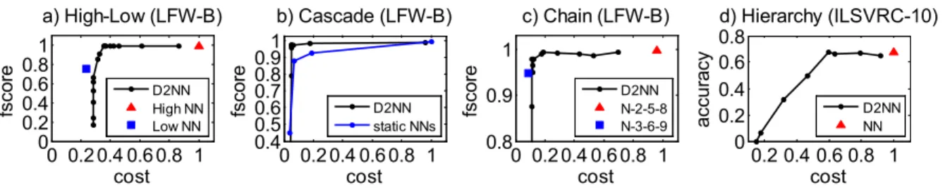
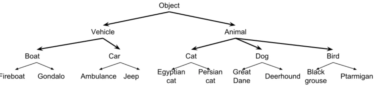
2.1 Two D2NN examples. Input and output nodes are drawn as circles with the output nodes shaded. Function nodes are drawn as rectangles (regular nodes) or diamonds (control nodes). Dummy nodes are shaded. Data edges are drawn as solid arrows and control edges as dashed arrows. A data edge with a user defined default value is decorated with a circle. . . 11 2.2 The accuracy-cost or fscore-cost curves of various D2_{NN architectures, as well as}

conventional DNN baselines consisting of only regular nodes. . . 20 2.3 Four different D2NN architectures. . . 21 2.4 Distribution of examples going through different execution paths. Skipped nodes are

in grey. The hyperparameterλcontrols the trade-off between accuracy and efficiency. A biggerλ values accuracy more. Left: for the high-low capacity D2NN. Right: for the hierarchical D2_{NN. The X-axis is the number of nodes activated.} _{. . . .} ₂₄ 2.5 Examples with different paths in a high-low D2NN (left) and a hierarchical D2NN

(right). . . 24 2.6 Accuracy-cost curve for a chain D2_{NN on the CMNIST task compared to DCN. . . . .} ₂₅ 2.7 The semantic class hierarchy of the ILSVRC-10 dataset. . . 29 3.1 Computation graphs for conventional losses and UniLoss. Top: (a) testing for

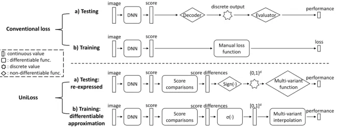
conven-tional losses. The decoder and evaluator are usually non-differentiable. (b) training for conventional losses. To avoid the non-differentiability, conventional methods op-timize a manually-designed differentiable loss function instead during training. Bot-tom: (a) refactorized testing in UniLoss. We refactorize the testing so that the non-differentiability exists only in Sign(·) and the multi-variant function. (b) training in UniLoss with the differentiable approximation of refactorized testing. σ(·)is the sig-moid function. We approximate the non-differentiable components in the refactorized testing pipeline with interpolation methods. . . 36 4.1 DetectorGAN generates object-inserted images as synthesized data to improve the

de-tection performance. DetectorGAN integrates a detector into the generator-discriminator loop. . . 59 4.2 The illustration for Eqn. 4.3 – unrolling one forward-backward pass for trainingDET

to bridge the link betweenGX and LrealDet (detection loss on real images). Detection

loss on real images has no direct link to the generatorGX. Last step of training old

DET (noted asDET0 in the figure, refers to sameDET module but in the previous training step) is unrolled as in the dotted rectangle. The red arrow represents the fact that there is a differentiable link betweenGX andLrealDet after the unrolling. . . 65

(9)

4.3 Example generated images from CycleGAN and DetectorGAN for NIH. The details are high-lighted in green boxes (added for visualization). Both methods generate syn-thetic images from clean images and bounding box masks. DetectorGAN generates nodule inserted images with better local and global quality. . . 69 4.4 Examples of generated synthetic images from PS-GAN and DetectorGAN. The

de-tails are high-lighted in green boxes (added for visualization). We see qualitative improvement for pedestrian task as well. . . 69 4.5 Comparison showing that adding synthetic images can help detect nodules in NIH

Chest X-ray more accurately. Here, green boxes are ground truth and red are predic-tions. . . 70 5.1 Overview of the Dynamically Grown GAN.Bottom: The dynamic growing process.

We alternate between growing the architecture and training the weights of the new architectures. Each growing step chooses among actions including growing the gen-erator (G) with a certain convolution layer, or growing discriminator (D) with a certain convolution layer, or growing both G and D to a higher resolution. In each training step, the new architectures inherit the weights from the old architectures.Top: Exam-ples of growing steps. . . 81 5.2 Examples of generated LSUN Images by ProgGAN and our DGGAN at 256×256

resolution. Top: ProgGAN, obtained from their paper. It is not stated whether it is randomly generated;Bottom: Our DGGAN, randomly generated. . . 88 5.3 Examples of generated CIFAR-10 Images by ProgGAN, AutoGAN and our DGGAN,

from left to right. ProgGAN and our DGGAN are randomly generated. AutoGAN images are obtained from their paper, which is also randomly generated. . . 88 5.4 G-to-D number of parameters ratio and normalized FID for candidates on CIFAR-10.

Left: all the candidates. Right: zoom-in to candidates with normalized FID smaller than 1.2. The red arrows show the growing process of the best performing GAN. . . . 92 5.5 How each action affects training, i.e. how much is the improvement of normalized

FID over parent. Actions include “Upscale”, which means increasing the resolution of both G and D by 2, “G, a, b”, which means growing a layer in G with a as filter size and b as number of filters, “D, a, b”, which means growing a layer in D with a as filter size and b as number of filters. Top: Percentage of candidates with positive improvement over parent after each action. Bottom: Average and standard deviation of the improvement for each action. . . 92 5.6 Left: How likely good/sub-optimal parent candidates result in good child candidates

with different normalized FID thresholds. The good candidates given a threshold are defined as candidates with normalized FID larger than the threshold and the sub-optimal ones are lower than the threshold. Each threshold holds for both parent can-didates and child cancan-didates.RightSimulation with different hyper-parameterspand

K. . . 93 5.7 Left: G-to-D number of parameters ratio and normalized FID for all the candidates in

(10)

5.8 How each action affects training, i.e. how much is the improvement of normalized FID over parent. Top: Percentage of candidates with positive improvement over parent after each action. Bottom: Average and standard deviation of the improvement for each action. . . 97 5.9 Left: How likely good/sub-optimal parent candidates result in good child candidates

with different normalized FID thresholds. Right: Simulation with different hyper-parameterspandK. . . 97

(11)

LIST OF TABLES

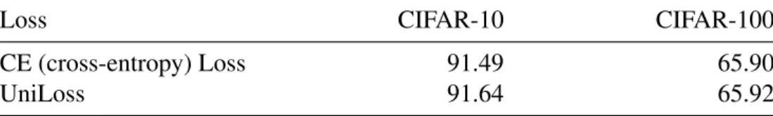
3.1 PCKh of Stacked Hourglass with MSE and UniLoss on the MPII validation. . . 51 3.2 Accuracy of ResNet-20 with CE loss and UniLoss on the CIFAR-10 and CIFAR-100

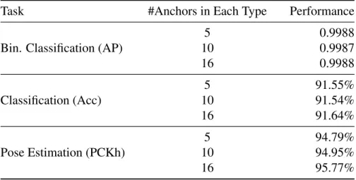
test set. . . 52 3.3 Ablation study for mini-batch sizes on CIFAR-10. . . 53 3.4 Ablation study for number of anchors on the three tasks. . . 53 4.1 Nodule AP on expanded annotation setting on the test set with IoU = 0.1 for NIH.

Baseline is using only real training data. We add 1000 synthetic images from Cycle-GAN and Cycle-GAN-D for training. . . 67 4.2 Localization accuracy with differentTIOU on “old annotations” test set for NIH. The

latter three uses RetinaNet as the model. . . 67 4.3 Localization accuracy with differentTIOBB on the “old annotations” test set on NIH. . 70

4.4 User study on the NIH Chest X-ray dataset. . . 70 4.5 Pedestrian detection AP trained with real data, synthetic data generated by PS-GAN,

pix2pix and DetectorGAN. . . 74 5.1 Quantitative evaluation on CIFAR-10, compared with ProgGAN at each resolution. . . 86 5.2 Quantitative evaluation on CIFAR-10, compared to prior state-of-the-art works. Top:

manually-designed GANs. Bottom: automatic GANs. Lower FID and higher Incep-tion Score indicate better generaIncep-tion quality. . . 86 5.3 Quantitative evaluation on LSUN, compared with ProgGAN at each scale. . . 89 5.4 Quantitative evaluation on LSUN, compared to prior state-of-the-art works. SWD

averages over multiple feature scales from 256 to 16. Lower FID and smaller SWD indicate better generation quality. All methods except COCO-GAN are non part-based GANs that learns to generate the whole images. COCO-GAN learns to generate parts of images instead. . . 89

(12)

ABSTRACT

To train a Deep Neural Network (DNN) that performs well for a task, many design steps are taken including data designs, model designs and loss designs. Despite that remarkable progress has been made in all these domains of designing DNNs, the unexplored design space of each com-ponent is still vast. That brings the research field of developing automated techniques to lift some heavy work from human researchers when exploring the design space. The automated designs can help human researchers to make massive or challenging design choices and reduce the expertise required from human researchers.

Much effort has been made towards automated designs of DNNs, including synthetic data generation, automated data augmentation, neural architecture search and so on. Despite the huge effort, the automation of DNN designs is still far from complete. This thesis contributes in two ways: identifying new problems in the DNN design pipeline that can be solved automatically, and proposing new solutions to problems that have been explored by automated designs.

The first part of this thesis presents two problems that were usually solved with manual designs but can benefit from automated designs. To tackle the problem of inefficient computation due to using a static DNN architecture for different inputs, some manual efforts have been made to use different networks for different inputs as needed, such as cascade models. We propose an automated dynamic inference framework that can cut this manual effort and automatically choose different architectures for different inputs during inference. To tackle the problem of designing differentiable loss functions for non-differentiable performance metrics, researchers usually design the loss manually for each individual task. We propose an unified loss framework that reduces the amount of manual design of losses in different tasks.

(13)

au-tomated design has been shown effective. In the synthetic data generation domain, we propose a novel method to automatically generate synthetic data for small-data object detection. The syn-thetic data generated can amend the limited annotated real data of the small-data object detection tasks, such as rare disease detection. In the architecture search domain, we propose an architec-ture search method customized for generative adversarial networks (GANs). GANs are commonly known unstable to train where we propose this new method that can stabilize the training of GANs in the architecture search process.

(14)

CHAPTER 1

Introduction

1.1

Background: Design in Deep Neural Networks

With the big success of deep neural networks (DNNs) in vision, language, recommendation and many other Machine Learning (ML) fields, lots of efforts are put into designing deep neural network models that perform better, in terms of better accuracy, efficiency, and generalization ability. To train a DNN that performs well for a task, especially a supervised task, designing the DNN architecture is not the only step. It starts from data collection where we collect raw data such as images, videos or words from all kinds of sources, and human workers annotate the collected data with the desired labels. We also augment the data with flipping, re-scaling and more to improve the generalization ability. Next, we design the architecture of the DNN to train. We also design a loss function and choose the optimization method and hyper-parameters. Finally, when we deploy the trained model to certain applications, we may use the trained DNN with certain post-processing steps and evaluate it with the performance metrics that we care about.

The whole pipeline can be categorized into three types of designs: data design, model de-sign and loss dede-sign. More specifically, the data dede-sign include data collection, data annotation, data augmentation etc. The model design include architecture design, network compression, etc. The loss design include differentiable loss function design, optimization method design, hyper-parameters exploration and so on.

In each line of work, enormous new works have been proposed in recent years. For example, in data design, data augmentation techniques (Xu et al., 2016; Perez and Wang, 2017) improve the

(15)

generalization ability of DNNs significantly; hard-example mining techniques (Shrivastava et al., 2016; Loshchilov and Hutter, 2015) improve effective use of data in unbalanced data situations.

In model design, revolutionary architectures have been proposed, including Inception-Net (Szegedy et al., 2015), residual networks (He et al., 2016), dense networks (Huang et al., 2017) and so on. To address the issue that networks are sometimes too computationally expensive for edge devices, net-work compression (Han et al., 2015; Denton et al., 2014; Chen et al., 2014; Gupta et al., 2015) and conditional computation (Bengio et al., 2015, 2013; Shazeer et al., 2017) techniques are proposed. In loss design, with a large amount of new tasks emerging, exploration for both using existing loss functions for newer tasks or developing new loss functions is conducted (Taylor et al., 2008; Henderson and Ferrari, 2016; Liu et al., 2016). In addition, new optimization methods (Reddi et al., 2018; Kingma and Ba, 2015; Loshchilov and Hutter, 2019; Ma and Yarats, 2019) and hyper-parameter tuning techniques (Bergstra et al., 2011; Bardenet et al., 2013) are proposed for faster and better optimization of the losses.

1.2

Motivation

Despite that remarkable progress has been made in all these domains of designing DNNs, the unexplored design space of each component is still vast. With the deep neural networks helping to lift some tiring and massive work from human workers, for example automatically detecting irregular events, classifying inappropriate entertainment content, a natural question arises: can we also develop automated techniques to lift some heavy work from human researchers when exploring the design space of the deep neural networks?

This is one of the biggest motivations behind this thesis. We expect automated design of deep neural networks can help lift the heavy work from human researchers in two aspects:

1. Automated design help human researchers to make massive or challenging design choices; 2. Automated design reduce the expertise required for human researchers.

(16)

Massive or Challenging Design Choices In each component of the DNN training, there remains large unexplored design spaces. To explore them, massive work that shares certain similar sub-processes needs to be done. With those sub-sub-processes automated and even smartly-oriented, the labor of human researchers can be freed.

For example, in architecture design, there is a big space to choose which layers to have and how to connect layers. Automated design can be used to explore these choices. Neural Architecture Search (NAS) (Zoph et al., 2018; Zoph and Le, 2017) explores to search over these choices to construct neural networks for various tasks, including image classification (Real et al., 2019; Liu et al., 2019b, 2018), segmentation (Liu et al., 2019a; Chen et al., 2018), and others (So et al., 2019; Wong et al., 2018).

In addition to architecture design, other design choices such as hyper-parameters, can also be explored automatically (Snoek et al., 2015; Domhan et al., 2015).

There are also design decisions where it is challenging to accomplish with only human labors. For example, training data is often obtained by many human annotators collecting and annotating data. However, sometimes obtaining training data is challenging, either due to the rarity of the data itself, or difficulties to obtain high quality data. One common example is to collect medical related images – some diseases are naturally rare to observe, and to annotate these images, well-trained medical specialists is needed. In such cases, methods such as the automatic annotation (Murthy et al., 2015), synthetic data generation (Liang et al., 2017; Gurumurthy et al., 2017; Li et al., 2017a; Yang and Deng, 2018) are used to help.

Human Expertise Automated design can also reduce the level of expert knowledge required. For example, many of the model design require human expertise, such as how to choose model capacity with different amounts of data and how to select thresholds for cascade models. With the automated neural architecture search and hyper-parameter tuning techniques, less expertise is needed to train a model. For example, sometimes a simple start button can do all the hyper-parameter tuning process. This further enables broader application of DNNs in various domains. A

(17)

typical application case is the AutoML service in the cloud industry, where small business holders are able to train image classifiers for their own business needs.

In loss design, to optimize for non-differentiable performance metrics that we care about, re-searchers often need to propose differentiable surrogate losses for network training. However, de-signing surrogate losses can sometimes incur substantial manual effort, including a large amount of the trial and error and the hyper-parameter tuning. This effort is important because a poorly designed loss can be misaligned with the final performance metric and lead to ineffective training. Automated design of surrogate losses such as learning to learn (Li and Malik, 2017; Chen et al., 2017) helps to reduce the level of expert knowledge required.

1.3

Contributions

Recent works towards automated design of DNNs include synthetic data generation, automated annotation, automated data augmentation, neural architecture search, automated hyper-parameter tuning and so on. Despite the huge effort, the automation of DNN design is still far from com-plete. Towards automated design of DNNs, this thesis contributes in two ways: 1) identifying new problems in the DNN design pipeline that can be solved automatically, such as automated dynamic inference and unified loss, and 2) proposing new solutions to problems that have been explored by automated designs, such as synthetic data generation and architecture search.

We identify problems that were usually solved with manual design but can benefit from auto-mated design.

• To tackle the problem of inefficient computation due to using a static DNN architecture for different inputs, some manual efforts have been made to use different networks for differ-ent inputs as needed, such as cascade models. We propose the first automated dynamic inference framework that can cut this manual effort and automatically choose different ar-chitectures for different inputs during inference.

(18)

per-formance metrics, manual trials are made for each task by researchers. We propose the first unified lossframework that reduces the amount of manual design of losses in different tasks. We also make efforts towards developing new techniques in domains where the automated design has been shown effective.

• Insynthetic data generationdomain, we propose a novel method to automatically generate synthetic data for small-data object detection.

• Inarchitecture search domain, we propose an architecture search method customized for Generative Adversarial Networks (GANs).

1.4

Thesis Outline

This thesis first summarizes our motivation and contributions in Chapter 1. Chapter 2-5 il-lustrate in detail about the particular problems in automated design that we are solving and the solutions we propose. Chapter 6 further discusses the limitations and future works.

1.4.1

Automated Dynamic Inference (Chapter 2)

In this chapter, we use automated design to address the problem of unnecessary computation in inference. During the inference of a DNN model, the same amount of computation is used for every input because the DNN is static. However, this is often not necessary because each input may require different amounts of computation to be classified correctly (some are difficult to classify but some are easy). Manual efforts such as cascade models are used to reduce unnecessary computation in the past. Instead of manually-designed cascades, we introduce Dynamic Deep Neural Networks (D2_{NN), a new type of feed-forward deep neural network that allows automatic dynamic inference.} That is, given an input, only a subset of D2_{NN neurons are executed, and the particular subset is} determined by the D2NN itself automatically. By pruning unnecessary computation depending on input, D2NNs provide a way to improve computational efficiency. With extensive experiments of various D2NN architectures on image classification tasks, we demonstrate that D2NNs are general

(19)

and flexible, and can effectively improve computational efficiency during inference. This chapter is based on a joint work with Jia Deng (Liu and Deng, 2018).

1.4.2

Unified Loss Design (Chapter 3)

In this chapter, we use automated design to reduce the manual efforts needed to design loss functions. The target performance metric for a task is often non-differentiable with respect to the DNN parameters. We thus need to design trainable surrogate losses that are differentiable and properly approximating the performance metrics. Large amount of manual effort is needed to de-sign task-specific surrogate losses. To reduce this manual effort, we introduce UniLoss, a unified framework to generate surrogate losses for training deep networks with gradient descent. Our key observation is that in many cases, evaluating a model with a performance metric on a batch of examples can be refactored into four steps: from input to real-valued scores, from scores to com-parisons of pairs of scores, from comcom-parisons to binary variables, and from binary variables to the final performance metric. Using this refactorization we generate differentiable approximations for each non-differentiable step through interpolation. Using UniLoss, we can optimize for differ-ent tasks and metrics using one unified framework, achieving comparable performance compared with manually-designed losses. This chapter is based on a joint work with Mingzhe Wang and Jia Deng (Liu et al., 2020a).

1.4.3

Synthetic Data Generation for Small-data Object Detection (Chapter 4)

In this chapter, we explore a new method in synthetic data generation, where we generate synthetic data to amend real data collected by human annotators. In particular, we explore object detection in the small data regime, where only a limited number of annotated bounding boxes are available due to data rarity and annotation expense. We address this problem by learning to generate new synthetic images with associated bounding boxes, and using these for training an object detector. We show that simply training previously proposed generative models does not yield satisfactory performance due to them optimizing for image realism rather than object

(20)

detection accuracy. To this end we develop a new model with a novel unrolling mechanism that jointly optimizes the generative model and a detector such that the generated images improve the performance of the detector. We show this method outperforms the state of the art on two challenging datasets, disease detection and small data pedestrian detection. This chapter is based on a joint work with Michael Muelly, Jia Deng, Tomas Pfister and Li-Jia Li (Liu et al., 2019c).

1.4.4

Architecture Search for GANs (Chapter 5)

In this chapter, we explore a new strategy in architecture search domain. While architecture search methods have been successfully applied in many problems, little effective effort has been made for GANs, especially considering the difficulties and instabilities to train large-scale GANs. In light of the recent work introducing progressive network growing as a promising way to ease the training for large GANs, we propose a method to dynamically grow GANs during training, opti-mizing the network architecture and its parameters together with automation. The method embeds architecture search techniques as an interleaving step with gradient-based training to periodically seek the optimal architecture-growing strategy for the generator and discriminator. It enjoys the benefits of both eased training because of the progressive growing and improved performance be-cause of the broader architecture design space. Experimental results demonstrate state-of-the-art of image generation. Observations in the search procedure also provide constructive insights into the GAN model design such as the generator-discriminator balance and convolutional layer choices. This chapter is based on a joint work with Yuting Zhang, Jia Deng and Stefano Soatto (Liu et al., 2020b).

1.5

Related Work

1.5.1

Automated Data Design

With the enormous progress in the data design, especially in constructing larger and larger datasets (Deng et al., 2009; Lin et al., 2014; Cordts et al., 2016), automated assistance to obtain

(21)

and annotate data becomes essential. Automatic annotationtechniques (Murthy et al., 2015) have been developed to reduce the workload to manually annotate data with human labors. Synthetic data generationis one of the techniques to automatically obtain clean and annotated data in many domains including 3D reconstruction, semantic segmentation, object detection and so on (Liang et al., 2017; Gurumurthy et al., 2017; Li et al., 2017a; Yang and Deng, 2018). As the first few to explore synthetic data generation for the small-data object detection task, we propose a GAN-based method that is fundamentally different from previous work—we construct a direct feedback link between the image generator and the object detector while previous work has no such feedback.

1.5.2

Automated Model Design

Neural Architecture Search(NAS) (Zoph et al., 2018; Zoph and Le, 2017) explores to search neural network architectures for various tasks, including image classification (Real et al., 2019; Liu et al., 2019b, 2018), segmentation (Liu et al., 2019a; Chen et al., 2018), image generation with GANs (Wang and Huan, 2019; Gong et al., 2019) and others (So et al., 2019; Wong et al., 2018). For architecture search of GANs, we propose a new method that combines progressive growing with architecture search. Our new method is thus able to search for high-resolution (256×256) GANs while previous work (Wang and Huan, 2019; Gong et al., 2019) can search for only lower resolution (up to 48×48) GANs.

Most of these works focus on the accuracy performance. To improve the efficiency perfor-mance of neural networks, learned network compression (Han et al., 2015; Denton et al., 2014; Chen et al., 2014; Gupta et al., 2015) is proposed to eliminate redundancy in data or computa-tion in a way that is input-independent. Also,conditional computation(Bengio et al., 2015, 2013; Shazeer et al., 2017) techniques are proposed to perform input-dependent pruning of the network. Along the line of input-dependent computation saving, we propose a new framework with auto-matic dynamic inference: with a large computation graph, the inference of each image involves a dynamic part of the computation graph and which part is determined by the model itself.

(22)

1.5.3

Automated Loss Design

Automated design of surrogate losses of non-differentiable performance metrics is proposed to ease the design process and reduce the level of expert knowledge required. Reinforcement learning algorithms have been also used to optimize performance metrics for structured output problems, especially those that can be formulated as taking a sequence of actions (Ranzato et al., 2016; Liu et al., 2017b; Caicedo and Lazebnik, 2015; Yeung et al., 2016; Zhou et al., 2018). Learning to learn methods (Li and Malik, 2017; Chen et al., 2017) use neural networks to learn a loss function using output-performance data pairs. We provide a new framework to propose surrogate losses in a unified way that does not involve substantial task-specific designs. It does not involve learning parameters as learning to learn methods or formulating the task as a sequence of actions as reinforcement learning methods.

In addition, automatic hyper-parameter tuning techniques (Snoek et al., 2015; Domhan et al., 2015) are proposed for faster and better optimization of the losses.

(23)

CHAPTER 2

Automated Dynamic Inference

1

2.1

Introduction

In this chapter, we address the problem of unnecessary computation in inference. There has been need for inference computational efficiency, in particular, by the need to deploy deep networks on mobile devices and data centers. Mobile devices are constrained by energy and power, limiting the amount of computation that can be executed. Data centers need energy efficiency to scale to higher throughput and to save operating cost.

However, during the inference of a traditional DNN model, the same amount of computation is used for every input because the DNN is static. This is often not necessary because each input may requires different amount of computation to be classified correctly. For example, to classify whether an image contains a car or not, some images with a front view of the car may be easy to classify with a small network but some images with only a part of the car visible may be difficult and need a larger network.

Manual efforts such as cascade models (Li et al., 2015; Sun et al., 2013) are used to reduce un-necessary computation in the past. Instead of manually-designed cascades, we introduce Dynamic Deep Neural Networks (D2NN), a new type of feed-forward deep neural network that allows au-tomatic dynamic inference. That is, given an input, only a subset of neurons are executed, and the particular subset is determined by the network itself based on the particular input. In other words, the amount of computation and computation sequence are dynamic based on input. This is

(24)

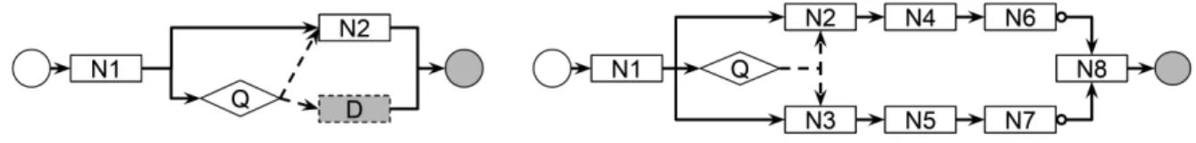
Figure 2.1: Two D2NN examples. Input and output nodes are drawn as circles with the output nodes shaded. Function nodes are drawn as rectangles (regular nodes) or diamonds (control nodes). Dummy nodes are shaded. Data edges are drawn as solid arrows and control edges as dashed arrows. A data edge with a user defined default value is decorated with a circle.

ferent from standard feed-forward networks that always execute the same computation sequence regardless of input.

A D2NN is a feed-forward deep neural network (directed acyclic graph of differentiable mod-ules) augmented with one or more control modules. A control module is a sub-network whose output is a decision that controls whether other modules can execute. Fig. 2.1 (left) illustrates a simple D2NN with one control module (Q) and two regular modules (N1, N2), where the controller Q outputs a binary decision on whether module N2 executes. For certain inputs, the controller may decide that N2 is unnecessary and instead execute a dummy node D to save on computation. As an example application, this D2_{NN can be used for binary classification of images, where some} images can be rapidly classified as negative after only a small amount of computation.

D2NNs provide a way to improve computational efficiency by selective execution, pruning unnecessary computation depending on input. D2NNs also make it possible to use a bigger network under a computation budget by executing only a subset of the neurons each time.

A D2NN is trained end to end. That is, regular modules and control modules are jointly trained to optimize both accuracy and efficiency. We achieve such training by integrating backpropagation with reinforcement learning, necessitated by the non-differentiability of control modules.

Compared to prior work that optimizes computational efficiency in computer vision and ma-chine learning, our work is distinctive in four aspects: (1) the decisions on selective execution are part of the network inference and are learned end to end together with the rest of the network, as opposed to hand-designed or separately learned (Li et al., 2015; Sun et al., 2013; Almahairi et al., 2016); (2) D2NNs allow more flexible network architectures and execution sequences

(25)

in-cluding parallel paths, as opposed to architectures with less variance (Denoyer and Gallinari, 2014; Shazeer et al., 2017); (3) our D2NNs directly optimize arbitrary efficiency metric that is defined by the user, while previous work has no such flexibility because they improve efficiency indirectly through sparsity constraints (Bengio et al., 2015, 2013; Shazeer et al., 2017). (4) our method op-timizes metrics such as the F-score that does not decompose over individual examples. This is an issue not addressed in prior work. We will elaborate on these differences in the Related Work section of this chapter.

We perform extensive experiments to validate our D2NNs algorithms. We evaluate various D2NN architectures on several tasks. They demonstrate that D2NNs are general, flexible, and can effectively improve computational efficiency.

Our main contribution is the D2_{NN framework that allows a user to augment a static} feed-forward network with control modules to achieve automated dynamic inference. We show that D2NNs allow a wide variety of topologies while sharing a unified training algorithm. To our knowledge, D2NN is the first single automated framework that can support various qualitatively different efficient network designs, including cascade designs and coarse-to-fine designs.

2.2

Related work

Input-dependent execution has been widely used in computer vision, from cascaded detec-tors (Viola and Jones, 2004; Felzenszwalb et al., 2010) to hierarchical classification (Deng et al., 2011; Bengio et al., 2010). The key difference of our work from prior work is that wejointlylearn both visual features and control decisionsend to end, whereas prior work either hand-designs fea-tures and control decisions (e.g. thresholding), or learns them separately.

In the context of deep networks, two lines of prior work have attempted to improve computa-tional efficiency. One line of work tries to eliminate redundancy in data or computation in a way that is input-independent. The methods include pruning networks (Han et al., 2015; Wen et al., 2016; Alvarez and Salzmann, 2016), approximating layers with simpler functions (Denton et al., 2014; Zhang et al., 2016), and using number representations of limited precision (Chen et al., 2014;

(26)

Gupta et al., 2015). The other line of work exploits the fact that not all inputs require the same amount of computation, and explores input-dependent execution of DNNs. Our work belongs to the second line, and we will contrast our work mainly with them. In fact, our input-dependent D2_{NN can be combined with input-independent methods to achieve even better efficiency.}

Among methods leveraging input-dependent execution, some use pre-defined execution-control policies. For example, cascade methods (Li et al., 2015; Sun et al., 2013) rely on manually-selected thresholds to control execution; Dynamic Capacity Network (Almahairi et al., 2016) designs a way to directly calculate a saliency map for execution control. Our D2NNs, instead, are fully learn-able; the execution-control policies of D2NNs do not require manual design and are learned together with the rest of the network.

Our work is closely related to conditional computation methods (Bengio et al., 2015, 2013; Shazeer et al., 2017), which activate part of a network depending on input. They learn policies to encourage sparse neural activations (Bengio et al., 2015) or sparse expert networks (Shazeer et al., 2017). Our work differs from these methods in several ways. First, our control policies are learned to directly optimize arbitrary user-defined global performance metrics, whereas conditional computation methods have only learned policies that encourage sparsity. In addition, D2NNs allow more flexible control topologies. For example, in (Bengio et al., 2015), a neuron (or block of neurons) is the unit controllee of their control policies; in (Shazeer et al., 2017), an expert is the unit controllee. Compared to their fixed types of controllees, our control modules can be added in any point of the network and control arbitrary subnetworks. Also, various policy parametrization can be used in the same D2NN framework. We show a variety of parameterizations (as different controller networks) in our D2NN examples, whereas previous conditional computation works have used some fixed formats: For example, control policies are parametrized as the sigmoid or softmax of an affine transformation of neurons or inputs (Bengio et al., 2015; Shazeer et al., 2017). Our work is also related to attention models (Denil et al., 2012; Mnih et al., 2014; Gregor et al., 2015). Note that attention models can be categorized as hard attention (Mnih et al., 2014; Ba et al., 2014; Almahairi et al., 2016) versussoft (Gregor et al., 2015; Stollenga et al., 2014). Hard

(27)

attention models only process the salient parts and discard others (e.g. processing only a subset of image subwindows); in contrast, soft attention models process all parts but up-weight the salient parts. Thus only hard attention models perform input-dependent execution as D2_{NNs do. However,} hard attention models differ from D2_{NNs because hard attention models have typically involved} only one attention module whereas D2_{NNs can have multiple attention (controller) modules —} conventional hard attention models are “single-threaded” whereas D2NN can be “multi-threaded”. In addition, prior work in hard attention models have not directly optimized for accuracy-efficiency trade-offs. It is also worth noting that many mixture-of-experts methods (Jacobs et al., 1991; Jordan and Jacobs, 1994; Eigen et al., 2013) also involve soft attention by soft gating experts: they process all experts but only up-weight useful experts, thus saving no computation.

D2_{NNs also bear some similarity to Deep Sequential Neural Networks (DSNN) (Denoyer and} Gallinari, 2014) in terms of input-dependent execution. However, it is important to note that al-though DSNNs’ structures can in principle be used to optimize accuracy-efficiency trade-offs, DSNNs are not for the task of improving efficiency and have no learning method proposed to optimize efficiency. And the method to effectively optimize for efficiency-accuracy trade-off is non-trivial as is shown in the following sections. Also, DSNNs are single-threaded: it always acti-vates exactly one path in the computation graph, whereas for D2NNs it is possible to have multiple paths or even the entire graph activated.

2.3

Definition and Semantics of D

2

NNs

Here we precisely define a D2_{NN and describe its semantics, i.e. how a D}2_{NN performs} infer-ence.

2.3.1

D

2

NN definition

A D2NN is defined as a directed acyclic graph (DAG) without duplicated edges. Each node can be one of the three types: input nodes, output nodes, and function nodes. An input or output node represents an input or output of the network (e.g. a vector). A function node represents

(28)

a (differentiable) function that maps a vector to another vector. Each edge can be one of the two types: data edges and control edges. A data edge represents a vector sent from one node to another, the same as in a conventional DNN. A control edge represents a control signal, a scalar, sent from one node to another. A data edge can optionally have a user-defined “default value”, representing the output that will still be sent even if the function node does not execute.

For simplicity, we have a few restrictions on valid D2NNs: (1) the outgoing edges from a node are either all data edges or all control edges (i.e. cannot be a mix of data edges and control edges); (2) if a node has an incoming control edge, it cannot have an outgoing control edge. Note that these two simplicity constraints do not in any way restrict the expressiveness of a D2NN. For example, to achieve the effect of a node with a mix of outgoing data edges and control edges, we can just feed its data output to a new node with outgoing control edges and let the new node be an identity function.

We call a function node a control node if its outgoing edges are control edges. We call a function node aregular node if its outgoing edges are data edges. Note that it is possible for a function node to take no data input and output a constant value. We call such nodes “dummy” nodes. We will see that the “default values” and “dummy” nodes can significantly extend the flexibility of D2NNs. Hereafter we may also call function nodes “subnetwork”, or “modules” and will use these terms interchangeably. Fig. 2.1 illustrates simple D2_{NNs with all kinds of nodes and} edges.

2.3.2

D

2

NN Semantics

Given a D2_{NN, we perform inference by traversing the graph starting from the input nodes.} Because a D2_{NN is a DAG, we can execute each node in a topological order (the parents of a} node are ordered before it; we take both data edges and control edges in consideration), same as conventional DNNs except that the control nodes can cause the computation of some nodes to be skipped.

(29)

outgo-ing control edges. The control edge with the highest score is “activated”, meanoutgo-ing that the node being controlled is allowed to execute. The rest of the control edges are not activated, and their controllees are not allowed to execute. For example, in Fig 2.1 (right), the node Q controls N2 and N3. Either N2 or N3 will execute depending on which has the higher control score.

Although the main idea of the inference (skipping nodes) seems simple, due to D2_NNs’ flex-ibility, the inference topology can be far more complicated. For example, in the case of a node with multiple incoming control edges (i.e. controlled by multiple controllers), it should execute if any of the control edges are activated. Also, when the execution of a node is skipped, its output will be either the default value or null. If the output is the default value, subsequent execution will continue as usual. If the output is null, any downstream nodes that depend on this output will in turn skip execution and have a null output unless a default value has been set. This “null” effect will propagate to the rest of the graph. Fig. 2.1 (right) shows a slightly more complicated exam-ple with default values: if N2 skips execution and outputs null, so will N4 and N6. But N8 will execute regardless because its input data edge has a default value. In our Experiments Section, we will demonstrate more sophisticated D2NNs.

We can summarize the semantics of D2NNs as follows: a D2NN executes the same way as a conventional DNN except that there are control edges that can cause some nodes to be skipped. A control edge is active if and only if it has the highest score among all outgoing control edges from a node. A node is skipped if it has incoming control edges and none of them is active, or if one of its inputs is null. If a node is skipped, its output will be either null or a user-defined default value. A null will cause downstream nodes to be skipped whereas a default value will not.

A D2NN can also be thought of as a program with conditional statements. Each data edge is equivalent to a variable that is initialized to either a default value or null. Executing a function node is equivalent to executing a command assigning the output of the function to the variable. A control edge is equivalent to a boolean variable initialized to False. A control node is equivalent to a “switch-case” statement that computes a score for each of the boolean variables and sets the one with the largest score to True. Checking the conditions to determine whether to execute a

(30)

function is equivalent to enclosing the function with an “if-then” statement. A conventional DNN is a program with only function calls and variable assignments without any conditional statements, whereas a D2_{NN introduces conditional statements with the conditions themselves generated by} learnable functions.

2.4

D

2

NN Learning

Due to the control nodes, a D2_{NN cannot be trained the same way as a conventional DNN. The} output of the network cannot be expressed as a differentiable function of all trainable parameters, especially those in the control nodes. As a result, backpropagation cannot be directly applied. The main difficulty lies in the control nodes, whose outputs are discretized into control decisions. This is similar to the situation with hard attention models (Mnih et al., 2014; Ba et al., 2014), which use reinforcement learning. Here we adopt the same general strategy.

2.4.1

Learning a Single Control Node

For simplicity of exposition we start with a special case where there is only one control node. We further assume that all parameters except those of this control node have been learned and fixed. That is, the goal is to learn the parameters of the control node to maximize a user-defined reward, which in our case is a combination of accuracy and efficiency. This results in a classical reinforcement learning setting: learning a control policy to take actions so as to maximize reward. We base our learning method on Q-learning (Mnih et al., 2013; Sutton and Barto). We let each outgoing control edge represent an action, and let the control node approximate the action-value (Q) function, which is the expected return of an action given the current state (the input to the control node).

It is worth noting that unlike many prior works that use deep reinforcement learning, a D2_NN is not recurrent. For each input to the network (e.g. an image), each control node only executes once. And the decisions of a control node completely depend on the current input. As a result, an action taken on one input has no effect on another input. That is, our reinforcement learning

(31)

task consists of only one time step. Our one time-step reinforcement learning task can also be seen as a contextual bandit problem, where the context vector is the input to the control module, and the arms are the possible action outputs of the module. The one time-step setting simplifies our Q-learning objective to that of the following regression task:

L= (Q(s,a)−r)2, (2.1)

whereris a user-defined reward,ais an action,sis the input to control node, andQis computed by the control node. As we can see, training a control node here is the same as training a network to predict the reward for each action under an L2 loss. We use mini-batch gradient descent; for each training example in a mini-batch, we pick the action with the largestQ, execute the rest of the network, observe a reward, and perform backpropagation using the L2 loss in Eqn. 2.1.

During training we also perform-greedy exploration — instead of always choosing the action with the best Q value, we choose a random action with probability . The hyper-parameter

is initialized to 1 and decreases over time. The reward r is user defined. Since our goal is to optimize the trade-off between accuracy and efficiency, in our experiments we define the reward as a combination of an accuracy metricA (for example, F-score) and an efficiency metricE (for example, the inverse of the number of multiplications), that is,λA+ (1−λ)E whereλbalances the trade-off.

2.4.2

Mini-Bags for Set-Based Metrics

Our training algorithm so far has defined the state as a single training example, i.e., the control node takes actions and observes rewards on each training example independent of others. This setup, however, introduces a difficulty for optimizing for accuracy metrics that cannot be decom-posed over individual examples.

Consider precision in the context of binary classification. Given predictions on a set of ex-amples and the ground truth, precision is defined as the proportion of true positives among the

(32)

predicted positives. Although precision can be defined on a single example, precision on a set of examples does not generally equal the average of the precisions of individual examples. In other words, precision as a metric does not decompose over individual examples and can only be com-puted using a set of examplesjointly. This is different from decomposable metrics such aserror rate, which can be computed as the average of the error rates of individual examples. If we use precision as our accuracy metric, it is not clear how to define a reward independently for each example such that maximizing this reward independently for each example would optimize the overall precision. In general, for many metrics, including precision and F-score, we cannot com-pute them on individual examples and average the results. Instead, we must comcom-pute them using a set of examples as a whole. We call such metrics “set-based metrics”. Our learning setup so far is ill-equipped for such metrics because a reward is defined on each example independently.

To address this issue we generalize the definition of a state from a single input to a set of inputs. We define such a set of inputs as amini-bag. With a mini-bag of images, any set-based metric can be computed and can be used to directly define a reward. Note that a mini-bag is different from a mini-batch which is commonly used for batch updates in gradient decent methods. Actually in our training, we calculate gradients using a mini-batch of mini-bags. Now, an action on a mini-bag

s = (s1, . . . , sm) is now a joint action a = (a1, . . . , am) consisting of individual actions ai on

examplesi. LetQ(s,a)be thejointaction-value function on the mini-bagsand the joint actiona.

We constrain the parametric form ofQto decompose over individual examples:

Q=

m X

i=1

Q(si, ai), (2.2)

whereQ(si, ai)is a score given by the control node when choosing the action ai for examplesi.

We then define our new learning objective on a mini-bag of sizemas

L= (r−Q(s,a))2 = (r− m X

i=1

Q(si, ai))2, (2.3)

(33)

0 0.20.4 0.60.8 1 0 0.2 0.4 0.6 0.81 a) High-Low (LFW-B) cost fsco re D2NN High NN Low NN 0 0.20.4 0.60.8 1 0.4 0.5 0.6 0.7 0.8 0.91 b) Cascade (LFW-B) cost fsco re D2NN static NNs 0 0.20.4 0.60.8 1 0.8 0.9 1 c) Chain (LFW-B) cost fsco re D2NN N-2-5-8 N-3-6-9 0.2 0.4 0.6 0.8 1 0 0.2 0.4 0.6 0.8 d) Hierarchy (ILSVRC-10) cost ac cur ac y D2NN NN

Figure 2.2: The accuracy-cost or fscore-cost curves of various D2NN architectures, as well as conventional DNN baselines consisting of only regular nodes.

node predicts an action-value for each example such that their sum approximates the reward defined on the whole mini-bag.

It is worth noting that the decomposition of Q into sums (Eqn. 2.2) enjoys a nice property: the best joint actiona∗ under the joint action-valueQ(s,a)is simply the concatenation of the best actions for individual examples because maximizing

a∗ = arg max a (Q(s,a)) = arg maxa ( m X i=1 Q(si, ai)) (2.4)

is equivalent to maximizing the individual summands:

a∗_i = arg max

ai

Q(si, ai), i= 1,2...m. (2.5)

That is, during test time we still perform inference on each example independently. Another implication of the mini-bag formulation is:

∂L ∂xi = 2(r− m X j=1 Q(sj, aj)) ∂Q(si, ai) ∂xi , (2.6)

where xi is the output of any internal neuron for example iin the mini-bag. This shows that

there is no change to the implementation of backpropagation except that we scale the gradient using the difference between the mini-bag Q-valueQand rewardr.

Joint Training of All Nodes We have described how to train a single control node. We now describe how to extend this strategy to all nodes including additional control nodes as well as

(34)

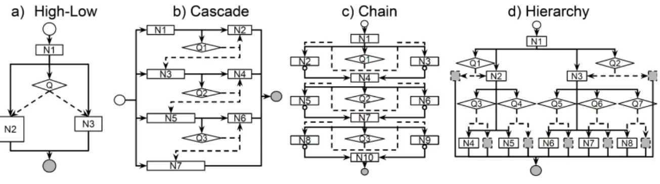
Figure 2.3: Four different D2_{NN architectures.}

regular nodes. If a D2NN has multiple control nodes, we simply train them together. For each mini-bag, we perform backpropagation for multiple losses together. Specifically, we perform inference using the current parameters, observe a reward for the whole network, and then use the same reward (which is a result of the actions of all control nodes) to backpropagate for each control node.

For regular nodes, we can place losses on them the same as on conventional DNNs. And we perform backpropagation on these losses together with the control nodes. The implementation of backpropagation is the same as conventional DNNs except that each training example have a different network topology (execution sequence). And if a node is skipped for a particular training example, then the node does not have a gradient from the example.

It is worth noting that our D2_{NN framework allows arbitrary losses to be used for regular nodes.} For example, for classification we can use the cross-entropy loss on a regular node. One important detail is that the losses on regular nodes need to be properly weighted against the losses on the control nodes; otherwise the regular losses may dominate, rendering the control nodes ineffective. One way to eliminate this issue is to use Q-learning losses on regular nodes as well, i.e. treating the outputs of a regular node as action-values. For example, instead of using the cross-entropy loss on the classification scores, we treat the classification scores as action-values—an estimated reward of each classification decision. This way Q-learning is applied to all nodes in a unified way and no additional hyperparameters are needed to balance different kinds of losses. In our experiments unless otherwise noted we adopt this unified approach.

(35)

2.5

Experiments

We here demonstrate four D2_{NN structures motivated by different demands of efficient network} design to show its flexibility and effectiveness, and compare D2NNs’ ability to optimize efficiency-accuracy trade-offs with prior work.

We implement the D2NN framework in Torch. Torch provides functions to specify the subnet-work architecture inside a function node. Our framesubnet-work handles the high-level communication and loss propagation.

2.5.1

High-Low Capacity D

2

NN

Our first experiment is with a simple D2NN architecture that we call “high-low capacity D2NN”. It is motivated by that we can save computation by choosing a low-capacity subnetwork for easy examples. It consists of a single control nodes (Q) and three regular nodes (N1-N3) as in Fig. 2.3a). The control node Q chooses between a high-capacity N2 and a low-capacity N3; the N3 has fewer neurons and uses less computation. The control node itself has orders of magnitude fewer compu-tation than regular nodes (this is true for all D2NNs demonstrated).

We test this hypothesis using a binary classification task in which the network classifies an input image as face or non-face. We use the Labeled Faces in the Wild (Huang et al., 2007; Learned-Miller, 2014) dataset. Specifically, we use the 13k ground truth face crops (112×112 pixels) as positive examples and randomly sampled 130k background crops (with an intersection over union less than 0.3) as negative examples. We hold out 11k images for validation and 22k for testing. We refer to this dataset as LFW-B and use it as a testbed to validate the effectiveness of our new D2NN framework.

To evaluate performace we measure accuracy using the F1 score, a better metric than percent-age of correct predictions for an unbalanced dataset. We measure computational cost using the number of multiplications following prior work (Almahairi et al., 2016; Shazeer et al., 2017) and for reproductivity. Specifically, we use the number of multiplications (control nodes included), normalized by a conventional DNN consisting of N1 and N2, that is, the high-capacity

(36)

execu-tion path. Note that our D2NNs also allow to use other efficiency measurement such as run-time, latency.

During training we define the Q-learning reward as a linear combination of accuracy A and efficiencyE (negative cost):r =λA+ (1−λ)Ewhereλ∈[0,1]. We train instances of high-low capacity D2_{NNs using different} _λ_{’s. As} _λ _{increases, the learned D}2_{NN trades off efficiency for} accuracy. Fig. 2.2a) plots the accuracy-cost curve on the test set; it also plots the accuracy and efficiency achieved by a conventional DNN with only the high capacity path N1+N2 (High NN) and a conventional DNN with only the low capacity path N1+N3 (Low NN).

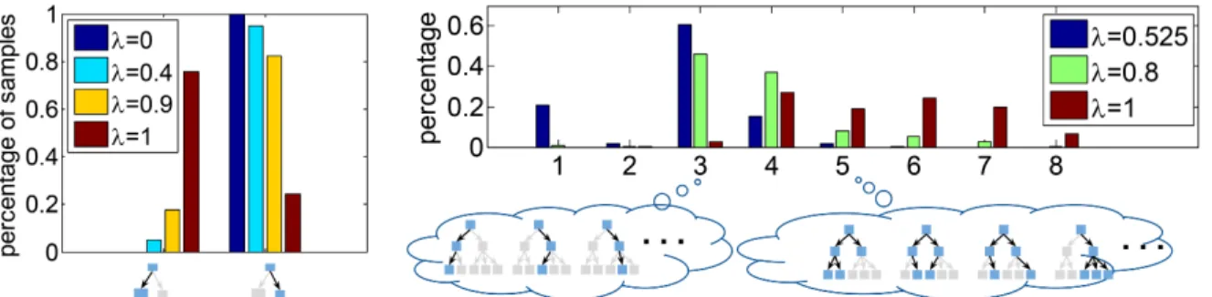
As we can see, the D2NN achieves a trade-off curve close to the upperbound: there are points on the curve that are as fast as the low-capacity node and as accurate as the high-capacity node. Fig. 2.4(left) plots the distribution of examples going through different execution paths. It shows that as λ increases, accuracy becomes more important and more examples go through the high-capacity node. These results suggest that our learning algorithm is effective for networks with a single control node.

With inference efficiency improved, we also observe that for training, a D2NN typically takes 2-4 times more iterations to converge than a DNN, depending on particular model capacities, con-figurations and trade-offs.

2.5.2

Cascade D

2

NN

We next experiment with a more sophisticated design that we call a “cascade D2NN” (Fig. 2.3b). It is inspired by the standard cascade design commonly used in computer vision. The intuition is that many negative examples may be rejected early using simple features. The cascade D2_NN consists of seven regular nodes (N1-N7) and three control nodes (Q1-Q3). N1-N7 form 4 cascade stages (i.e. 4 conventional DNNs, from small to large) of the cascade: N1+N2, N3+N4, N5+N6, N7. Each control node decides whether to execute the next cascade stage or not.

We evaluate the network on the same LFW-B face classification task using the same evaluation protocol as in the high-low capacity D2NN. Fig. 2.2b) plots the accuracy-cost tradeoff curve for the

(37)

Figure 2.4: Distribution of examples going through different execution paths. Skipped nodes are in grey. The hyperparameterλcontrols the trade-off between accuracy and efficiency. A biggerλ

values accuracy more. Left: for the high-low capacity D2_NN. _{Right: for the hierarchical D}2_NN. The X-axis is the number of nodes activated.

Figure 2.5: Examples with different paths in a high-low D2_{NN (left) and a hierarchical D}2_NN (right).

D2_{NN. Also included are the accuracy-cost curve (“static NNs”) achieved by the four conventional} DNNs as baselines, each trained with a cross-entropy loss. We can see that the cascade D2_NN can achieve a close to optimal trade-off, reducing computation significantly with negligible loss of accuracy. In addition, we can see that our D2NN curve outperforms the trade-off curve achieved by varying the design and capacity of static conventional networks. This result demonstrates that our algorithm is successful for jointly training multiple control nodes.

For a cascade, wall time of inference is often an important consideration. Thus we also measure the inference wall time (excluding data loading with 5 runs) in this Cascade D2_{NN. We find that a} 82% wall-time cost corresponds to a 53% number-of-multiplication cost; and a 95% corresponds to a 70%. Defining reward directly using wall time can further reduce the gap.

2.5.3

Chain D

2

NN

Our third design is a “Chain D2_{NN” (Fig. 2.3c). The network is shaped as a chain, where each} link consists of a control node selecting between two (or more) regular nodes. In other words, we perform a sequence of vector-to-vector transforms; for each transform we choose between several

(38)

0

2

4

6

8

x 10

7

0

0.2

0.4

0.6

0.8

1

#multiplications

ac

cu

ra

cy

D2NN

DCN

Figure 2.6: Accuracy-cost curve for a chain D2_{NN on the CMNIST task compared to DCN} (Alma-hairi et al., 2016).

subnetworks. One scenario that we can use this D2_{NN is that the configuration of a conventional} DNN (e.g. number of layers, filter sizes) cannot be fully decided. Also, it can simulate shortcuts between any two layers by using an identity function as one of the transforms. This chain D2_NN is qualitatively different from other D2NNs with a tree-shaped data graphbecause it allows two divergent data paths to merge again. That is, the number of possible execution paths can be exponential to the number of nodes.

In Fig. 2.3c), the first link is that Q1 chooses between a low-capacity N2 and a high-capacity N3. If one of them is chosen, the other will output a default value zero. The node N4 adds the outputs of N2 and N3 together. Fig. 2.2c) plots the accuracy-cost curve on the LFW-B task. The two baselines are: a conventional DNN with the lowest capacity path (N1-N2-N5-N8-N10), and a conventional DNN with the highest capacity path (N1-N3-N6-N9-N10). The cost is measured as the number of multiplications, normalized by the cost of the high-capacity baseline.

Fig. 2.2c) shows that the chain D2NN achieves a trade-off curve close to optimal and can speed up computation significantly with little accuracy loss. This shows that our learning algorithm is effective for a D2NN whose data graph is a general DAG instead of a tree.

2.5.4

Hierarchical D

2

NN

In this experiment we design a D2NN for hierarchical multiclass classification. The idea is to first classify images to coarse categories and then to fine categories. This idea has been explored

(39)

by numerous prior works (Liu et al., 2013; Bengio et al., 2010; Deng et al., 2011), but here we show that the same idea can be implemented via a D2NN trained end to end.

We use ILSVRC-10, a subset of the ILSVRC-65 (Deng et al., 2012). In ILSVRC-10, 10 classes are organized into a 3-layer hierarchy: 2 superclasses, 5 coarse classes and 10 leaf classes. Each class has 500 training images, 50 validation images, and 150 test images. As in Fig. 2.3d), the hierarchy in this D2NN mirrors the semantic hierarchy in ILSVRC-10. An image first goes through the root N1. Then Q1 decides whether to descend the left branch (N2 and its children), and Q2 decides whether to descend the right branch (N3 and its children). The leaf nodes N4-N8 are each responsible for classifying two fine-grained leaf classes. It is important to note that an input image can go down parallel paths in the hierarchy, e.g. descending both the left branch and the right branch, because Q1 and Q2 make separate decisions. This “multi-threading” allows the network to avoid committing to a single path prematurely if an input image is ambiguous.

Fig. 2.2d) plots the accuracy-cost curve of our hierarchical D2NN. The accuracy is measured as the proportion of correctly classified test examples. The cost is measured as the number of multiplications, normalized by the cost of a conventional DNN consisting only of the regular nodes (denoted as NN in the figure). We can see that the hierarchical D2NN can match the accuracy of the full network with about half of the computational cost.

Fig. 2.4(right) plots for the hierarchical D2_{NN the distribution of examples going through} exe-cution sequences with different numbers of nodes activated. Due to the parallelism of D2_{NN, there} can be many different execution sequences. We also see that asλincreases, accuracy is given more weight and more nodes are activated.

2.5.5

Comparison with Dynamic Capacity Networks

In this experiment we empirically compare our approach to closely related prior work. Here we compare D2NNs with Dynamic Capacity Networks (DCN) (Almahairi et al., 2016), for which efficency measurement is the absolute number of multiplications. Given an image, a DCN applies an additional high capacity subnetwork to a set of image patches, selected using a hand-designed

(40)

saliency based policy. The idea is that more intensive processing is only necessary for certain image regions.

To compare, we evaluate with the same multiclass classification task on the Cluttered MNIST (Mnih et al., 2014), which consists of MNIST digits randomly placed on a background cluttered with fragments of other digits. We train a chain D2_{NN of length 4 , which implements the same idea of} choosing a high-capacity alternative subnetwork for certain inputs. Fig. 2.6 plots the accuracy-cost curve of our D2NN as well as the accuracy-cost point achieved by the DCN in (Almahairi et al., 2016)—an accuracy of0.9861and and a cost of2.77×107. The closest point on our curve is an slightly lower accuracy of 0.9698 but slightly better efficiency (a cost of 2.66×107_{). Note that} although our accuracy of 0.9698 is lower, it compares favorably to those of other state-of-the-art methods such as DRAW (Gregor et al., 2015): 0.9664and RAM (Mnih et al., 2014):0.9189.

2.5.6

Visualization of Examples in Different Paths

In Fig. 2.5 (left), we show face examples in the high-low D2_{NN for}_λ_{=0.4. Examples in} low-capacity path are generally easier (e.g. more frontal) than examples in high-low-capacity path. In Fig. 2.5 (right), we show car examples in the hierarchical D2_{NN with 1) a single path executed} and 2) the full graph executed (for λ=1). They match our intuition that examples with a single path executed should be easier (e.g. less occlusion) to classify than examples with the full graph executed.

2.5.7

CIFAR-10 Results

We train a Cascade D2NN on CIFAR-10 where the corresponded DNN baseline is the ResNet-110. We initialize this D2NN with pre-trained ResNet-110 weights, apply cross-entropy losses on regular nodes, and tune the mixed-loss weight as explained in Sec. 4. We see a 30% reduction of cost with a 2% loss (relative) on accuracy, and a 62% reduction of cost with a 7% loss (relative) on accuracy. The D2_{NN’s ability to improve efficiency relies on the assumption that not all inputs} require the same amount of computation. In CIFAR-10, all images are low resolution (32 ×32),

(41)

and it is likely that few images are significantly easier to classify than others. As a result, the efficiency improvement is modest compared to other datasets.

2.6

Conclusion

In this chapter, we have introduced Dynamic Deep Neural Networks (D2NN), a new type of feed-forward deep neural networks that allow automated dynamic inference. Extensive experi-ments have demonstrated that D2NNs are flexible and effective.

2.7

Appendix

2.7.1

Implementation Details

We implement the D2NN framework in Torch. Torch already provides implementations of conventional neural network modules (nodes). So a user can specify the subnetwork architecture inside a control node or a regular node using existing Torch functionalities. Our framework then handles the communication between the user-defined nodes in the forward and backward pass.

To handle parallel paths, default-valued nodes and nodes with multiple data parents, we need to keep track of an example’s execution status (which nodes are activated by this example) and output status (which nodes have output for this example). An example’s output status is different from it