A new method for the assessment of spatial accuracy and completeness of OpenStreetMap building footprints

Article

A New Method for the Assessment of Spatial

Accuracy and Completeness of OpenStreetMap

Building Footprints

Maria Antonia Brovelli *ID _{and Giorgio Zamboni}

Department of Civil and Environmental Engineering (DICA), Politecnico di Milano, P.zza Leonardo Da Vinci 32, 20133 Milano, Italy; [email protected]

* Correspondence: [email protected]

Received: 29 April 2018; Accepted: 20 July 2018; Published: 24 July 2018 Abstract: OpenStreetMap (OSM) is currently the largest openly licensed collection of geospatial data, widely used in many projects as an alternative to or integrated with authoritative data. One of the main criticisms against this dataset is that, being a collaborative product created mainly by citizens without formal qualifications, its quality has not been assessed and therefore its usage can be questioned for some applications. This paper provides a map matching method to check the spatial accuracy of the building footprint layer, based on a comparison with a reference dataset. Moreover, from the map matching and a similarity check, buildings can be detected and therefore an index of completeness can also be computed. This process has been applied in Lombardy, a region in Northern Italy, covering an area of 23,900 km2and comprising respectively about 1 million buildings in OSM and 2.8 million buildings in the authoritative dataset. The results of the comparison show that the positional accuracy of the OSM buildings is at least compatible with the quality of the reference dataset at the scale of 1:5000 since the average deviation, with respect to the authoritative map, is below the expected tolerance of 3 m. The analysis of completeness, given in terms of the number of buildings appearing in the authoritative dataset and not present in OSM, shows an average percentage in the whole region equal to 57%. However, worth noting that the opposite, namely the number of buildings in OSM and not in the reference dataset, is not zero, but corresponds to 9%. The OSM building map can therefore be considered to be a valid base map for direct use (territorial frameworks, map navigation, urban analysis, etc.) and for derived use (background for the production of thematic maps) in all those cases where an accuracy corresponding to 1:5000 is required. Moreover it could be used for integrating the authoritative map at this scale (or smaller) where it is not complete and a rigorous quality certification in terms of metric precision is not required.

Keywords:GIS; digital cartography; algorithms; spatial accuracy; analysis; OpenStreetMap

1. Introduction

OpenStreetMap (OSM) [1] is currently the largest collaborative and openly licensed collection of geospatial data, widely used in many projects as an alternative to or integrated with authoritative data. OSM was founded in 2004 by Steve Coast as one of the first widespread efforts to provide a mapping platform for volunteered data capture [2]. It started as a mapping exercise for the United Kingdom but it spread quickly to the entire world. Coast’s idea was simple: combining worldwide local geographic data collected by a large number of widespread people who have local knowledge, makes it possible to build a geodatabase of the world [3].

In line with its collaborative mission, OSM data are available under the Open Database License [4]. Maps from OSM have a Creative Commons Attribution-ShareAlike 2.0 license (CC BY-SA) [5]. This

ISPRS Int. J. Geo-Inf.2018,7, 289 2 of 25

license allows everybody to use, distribute, transmit and adapt the data, as long as OSM and its contributors are credited. The license is viral: anyone who alters or builds upon OSM data must distribute the result only under the same license.

Currently, there are almost 4.5 million registered OSM members [6], more than 1 million contributors [7], and the impressive geospatial dataset is supported by software systems and applications, tools and web-based information stores such as wikis [3].

Many authors and commentators have concerned about the rapid and sustained success of OSM. One factor is certainly Web 2.0 [8], which makes it to develop large scale collaborative projects easier where hundreds or thousands of people are able to contribute simultaneously. A second factor is the availability of low-cost, high-quality, and high-accuracy positioning systems as standalone dedicated GPS units or embedded in portable devices such as smartphones. A third factor is related to the rising of so-called citizen science, i.e., scientific activities in which non-professional scientists volunteer to participate in data collection, analysis, and dissemination of a scientific project [9]. The volunteer practice and the outcome of the activities of OSM contributors, which are part of what is called volunteered geographic information (VGI) [10], can also be considered to be a component of “geographic” citizen science [9], both because of the scientific tools the volunteers make use of (remotely sensed images, GPS receivers, and map editing software) and the final collaborative aim they share, which is, mapping the Earth.

In turn, the phenomenon of citizen science can be seen as part of the new attitude towards more general open access, as well as collaborative and sharing approaches to information resources, which was named collective intelligence [11]. On the one side, this results in the willingness of citizens to participate in the knowledge production of the world; on the other side, these collaborative projects, of which OSM can be considered to be one of the most relevant examples, are inclusive and welcome anyone to take part in as a contributor, proposing a role and activities to everybody: beginners, expert level geographers, or software developers.

While the low level for entering and contributing has been one of the keys to the success of the initiative, the counterpoint is that, following a survey made by Budhathoki and Haythornthwaite [12], only 25% of the participants have “professional GIS experience” and therefore we are expecting a lower quality of the database compared with other sources, like data of national, regional and local mapping agencies as well as that produced by professionals and companies.

Some web tools are provided for mitigating and reducing errors. Examples related to geometry or topology are: the OSM Map Compare tool [13], which allows visual comparison of OSM map layers with other popular mapping systems such as Google maps [14], Bing maps [15], HERE maps [16], ESRI maps [17], etc.; Ma Visionneuse [18], which allows OSM to be compared with IGN (French National Institute of Geographic and Forest Information) France layers, amongst others; OSM Inspector [19], which shows potential errors like long segments in polygons and polylines, called “ways” in OSM, self-intersecting ways, polygons, or polylines which are represented by only one point, called “nodes” in OSM, and polygons or polylines containing duplicate nodes (for details about the topological model of OSM, see the following sections).

A useful application, named Taginfo [20] helps to check the tags and therefore the thematic quality. JOSM Validator [21] is a core feature of one of the most advanced editing tools of OSM. It checks and fixes a wide variety of problems, including topological errors, unclosed polygons and overlapping areas.

Osmose [22] and Keep Right [23] highlight errors in geometry/topology, tags, attribution, and other general OSM errors. MapRoulette [24] is a gamified application to fix errors in OSM. Each challenge proposes a set of tasks, which vary in difficulty, allowing contributors to choose the types of errors they feel more confident about fixing. DeepOSM [25] trains a neural network with OSM tags and aerial imagery, allowing the prediction of mis-registered roads in OSM. The Grass&Green project [26] is meant to correct tagging or classification of land use features involving grass or green areas.

Despite this huge number of applications for alleviating or correcting errors, some inaccuracies still remain and assessing the quality of the OSM spatial database is an issue on the agenda.

The ISO/TC 211 (technical committee) of the International Organization for Standardization (ISO) defines geographic information quality as the totality of characteristics of a product that bear on its ability to satisfy stated and implied needs. The quality measures that are considered for assessing VGI [27] are in general the most significant of the ISO 19157: 2013 Geographic Information—Data quality [28]: positional, thematic and temporal accuracy, completeness and consistency, even if there is still lack of formal standards for OSM.

“Accuracy” refers to the degree of closeness between a measurement of a quantity and the value which is accepted as true for that quantity. “Completeness” is assessed with respect to features, attributes, and model [29]. It can be evaluated in terms of commission errors, i.e., excess of data, and omission errors, i.e., absence of data. “Consistency” evaluates the coherence in the data structures; the errors resulting from the lack of it can be classified as referring to the conceptual model, domain, format and topology.

The assessment of OSM is a hot research topic and the majority of scholars have been contributing to this topic comparing the database against authoritative ones.

Hecht et al. [30], for instance, evaluated OSM building completeness in two regions of Germany applying different methods. The results highlighted a low degree of completeness, which was better in urban areas than rural areas, and also that the choice of method used for assessing the completeness has a high effect on the estimated value. Fan et al. [31], in comparing the building OSM dataset with the official one of Munich (Germany), found its high completeness over the city. However, with respect to the positional accuracy, the result was not so good as an average offset of about 4m exists between the two datasets. Conversely, they found that the footprints in the OSM dataset were highly similar to those in the reference dataset in terms of shape, the main difference being in fewer details (i.e., fewer points) in the polygons.

A different method, based on homologous point detection, was proposed by Brovelli et al. [32] on the city of Milan. The results seemed promising and the authors, considering also that there is not a consolidated and unique way for assessing spatial accuracy and completeness of the buildings dataset of OSM, decided to propose a new method and to test it on a significant case study covering the Italian region of Lombardy, which has an extent larger than the half of Switzerland and comprises both rural and highly populated urban areas. Moreover, as map matching approaches are more challenging in dense urban areas, where buildings are located close to each other and similar in shape and size [33], the authors also analyzed the outcomes focusing on the capitals of the provinces of the region.

The proposed methodology is partially derived from previous work of Brovelli and Zamboni [34,35] whose aim was authoritative map matching and warping. The method was based on the characteristics of the compared maps, specifically the existence of well-defined and rigorous prescriptions for their production. In this new approach, a different equality function was used because of the heterogeneity of the methods (and related accuracies) used by volunteers in collecting data.

The outcome of the paper is twofold: firstly, the presentation of the approach, which even though it still needs to be refined and compared to other methods, has good performance. Secondly, the evaluation of the positional accuracy and completeness of a significant dataset; the result on 940,000 buildings in the OSM map and about 2.8 million buildings in the Lombardy Regional Topographical Database (DBT) map shows that the quality of the OSM buildings is comparable to that of the regional technical authoritative map at the scale of 1:5000 everywhere, even in dense urban areas.

The remainder of this paper is structured as follows: Section2gives an overview of research related to this paper; Sections3and4respectively describe the method implemented for assessing the spatial accuracy and the completeness; Section5presents the results of the test areas, and Section6 summarizes the outcomes of the whole work and draws some activities for the future.

ISPRS Int. J. Geo-Inf.2018,7, 289 4 of 25

2. Related Work

As said, in recent years many researchers have been working on the assessment of OSM data. While significant attention has been paid to OSM positional accuracy assessment and completeness, fewer authors have investigated semantic, temporal and thematic accuracy, and consistency [36] and none, to the best of the authors’ knowledge, have assessed all the elements of data quality. As the method presented in the paper allows the assessment of positional accuracy and feature completeness, the analysis of the previous literature was mainly concentrated on these two aspects.

In the beginning, studies focused on the quality assessment of OSM road networks, which were the primary subjects of the OSM survey. The first studies date back to 2009. In their works, Ather [37], Haklay [38] and Koukoletsos et al. [39] assessed the positional accuracy of OSM streets in England (in an area corresponding to about 100 square kilometers) by a visual comparison of a limited number of roads with an authoritative dataset and a statistical approach based on a buffer technique developed by Goodchild and Hunter [40]. Moreover the completeness of the dataset over all England was estimated comparing the lengths of the roads in OSM with those of the Ordnance Survey vector datasets (the official dataset used for the assessment). Kounadi [41] did a similar experiment in Athens, where he considered around 300 roads and obtained results comparable to Hakley’s, i.e., an average difference between OSM and official roads of about 6 m and an average overlap of nearly 80%.

Cipeluch et al. [42] visually analyzed roads of five case study cities and towns in Ireland, finding slightly different results case by case, but highlighting that the OSM dataset merited attention if compared with other data, like the imagery available in Google Maps and Bing Maps. Moreover, they concluded that there is a need to develop metrics that allow the measurement of both accuracy and coverage at neighbourhood, county, and country levels so that the quality of the dataset can be quantified.

In the following years, other research studies were based on the buffer zone methodology [43–47]. The results are not homogeneous if we compare the different areas investigated. In Europe generally the spatial accuracy and the completeness were good enough, while in South Africa for instance, the dataset did not meet the accuracy requirements for the integration with the authoritative database. Al-Bakri and Fairbairn [48] assessed OSM in areas of England and Iraq by comparing reference survey data sets, and again the buffer method was used. They concluded that the integration of OSM data for large scale mapping applications was not viable.

Helbich et al. [49], in a case study of a city in Germany, used bi-dimensional regression analysis to evaluate the global geometries of the patterns and detected clusters of high and low precision by means of local autocorrelation statistics. They found that the OSM areas of high accuracy were primarily located in more populated parts of the city, leading to the conclusion that these areas were subject to more frequent validation, with consequent correction of errors, than rural areas.

Antoniou assessed the positional accuracy by evaluating, from geometry and semantics, the distance between corresponding intersections of the road network [50].

Girres and Touya [51] applied multiple methods to deal with the complexity of the analysis of the data, like the Euclidean distance for point features; the average Euclidean distance for linear features; the Hausdorff distance for linear features; and the surface distance, granularity, and compactness for area features. In their work, a limited number of homologous features, i.e., features representing the same object in the OSM and authoritative datasets, were selected and matched manually to avoid errors related to automatic processes. Differences in position were then computed on each pair of homologous objects. While the mean distance was acceptable, the standard deviation was definitely larger than the reference accuracy used for official datasets, showing that there was a huge heterogeneity in the quality of the data. Regarding completeness, they found that, using the number of objects as an indicator, OSM was far from being complete (around 10%); the completeness improved, however, when they considered the comparison between the total length/area of the objects, obtaining an average value of around 40%. This result clearly showed that shorter/smaller objects are more

likely to be absent, reflecting the fact that volunteer contributors tend to map the most important elements in the road network.

In 2013, Canavosio-Zuzelski et al. [52] proposed a rigorous photogrammetric approach based on stereo imagery and a vector adjustment model for assessing the positional accuracy of several OSM city streets. Forghani and Delavar [53] analyzed the data of one central urban zone of Tehran with a method combining different geometric elements—like road length, median center, minimum bounding geometry and directional distribution—concluding that the quality of OSM roads can be considered of medium level, mainly due to their heterogeneity. Brovelli et al. [54,55] introduced an automatic procedure based on geometrical similarity and a grid-based approach for the evaluation of road completeness and positional accuracy. The procedure was tested with good results on Paris, but it is completely flexible and can be reused by anybody because it is available as open source modules of the GIS GRASS [56].

The general comment about the assessment of OSM roads is that, even if many studies have been done, a general automatic solution does not yet exist and therefore there is still room in this field for investigating methods and developing new procedures.

Apart from the assessment of roads, in recent years researchers have also started assessing other objects in the OSM database, such as building footprints. To investigate the suitability of OSM data for the generation of 3D building models, Goetz and Zipf [57] provided a first quantitative analysis of OSM completeness, simply comparing the number of buildings mapped in OSM and the total number of buildings derived from the census data in Germany and showing that (in 2012) OSM covered around 30% of the total buildings. Hecht et al. [30] proposed four different methods for assessing the completeness with respect to the authoritative database: two respectively based on the comparison of building numbers and building areas calculated for reference unit zones (unit-based methods); and two respectively based on centroid and overlap for the detection of corresponding buildings in the two datasets (object-based methods). Their results indicated that the unit-based comparisons are highly sensitive to differences between the authoritative and the OSM data modeling, while object-based methods are more sensitive to positional mismatches of the OSM buildings. Anyhow, based on the analysis of many case studies, they concluded that object-based methods are preferable.

Fram et al. [58] assessed the quality of OSM buildings in different cities in the UK with the aim of investigating the potential of OSM data in applications of risk management solutions, such as natural catastrophe exposure models. The study was conducted applying the area unit-based method through a comparison against the authoritative datasets, and showed that OSM building completeness is very variable both within and between UK cities. Moreover, they tried to find a proxy variable for better computing the OSM completeness but they were not able to arrive at a satisfactory result.

Fan et al. [31] evaluated the quality of OSM in terms of completeness, semantic accuracy, positional accuracy, and shape accuracy by using building footprints of the official German dataset as reference data. Limiting the results to the indicators of interest for this paper, completeness was based on the area, identifying as corresponding objects those with an overlapping area that is larger than 30% of the smaller area of the two objects in OSM and the authoritative data. When one building of OSM matched only one building in the reference dataset (relation 1:1), the key points of the reference footprint were extracted using the Douglas-Peucker algorithm [59]. Next, the minimum bounding rectangles (MBRs) were calculated for the two polygons and their edges marked if they were located respectively on the edges of the corresponding MBR (OSM or reference). Again, the OSM MBR was shifted to the center of the reference MBR, in such a way that edges of these two MBRs could be matched if they were located (almost) on the same place. Finally, the edges of the footprints were matched if they were marked to the same edge of the MBRs. Regarding the positional accuracy, only buildings with a 1:1 relation were involved in the analysis and the accuracy was computed from the average distance between corresponding points in the pair of footprints in the two data sets. Finally, they also proposed computing the shape similarity between buildings, based on the turning function or tangent function introduced by Arkin et al. [60] for measuring the similarity of two polygons.

ISPRS Int. J. Geo-Inf.2018,7, 289 6 of 25

Törnros et al. [61] assessed OSM building completeness by comparison with a reference dataset, the official cadastre, and adopting the unit based method. However, they proposed a step forward with the computation of uncertainties given in terms of true positives, i.e., reference building areas that have been correctly mapped in OSM; false negatives, i.e., reference building areas not mapped in OSM; and false Positives, i.e., OSM building areas not mapped in the reference data set. Their conclusion was that it is best to adopt the true positive rate (building areas overlapping in OSM and the reference data) as a method for estimating the building completeness.

In the same year, Müller et al. [62], compared the OSM buildings with the authoritative ones in Switzerland with a procedure based on the respective centroid distance and the comparison of the shape signature based on the Arkin algorithm [60]. In more detail, the threshold of the centroid distance for correspondent buildings in the two datasets was set to 20 meters and the average of the turning function for matching buildings corresponded to around 1.25.

Finally, Brovelli et al. [32] assessed the completeness and the positional accuracy in Milan (Italy) using, for the former, the area unit based approach with the computation of uncertainties already seen in other studies, and, for the latter, a new method based on the automatic matching of the points of the footprints. The work presented here is a step forward in the definition of this second approach, which aims at contributing to the debate about positional accuracy and completeness of OSM, a debate that is still open.

3. Methodology: Spatial Accuracy

The assessment of the spatial accuracy proposed in this paper is based on the evaluation of the distance between points representing the same features in two different maps (or layers) depicting the same area. The implemented algorithm works on vector layers considering the vertices of the map features as a set of coordinates. In detecting the homologous entity (in our case the building footprint), the algorithm emulates what a human operator would do: it compares the position, the shape and the semantics of the features on the two maps.

Obviously, to find such a correspondence, the two maps must have more or less the same scale and they must show more or less the same level of detail (LoD).

In cartography the scale is a well-defined concept (“ratio of the length of an object on the map by the length of the same object on the ground”); conversely, LoD is a vague notion which can be considered as the translation of map scale for use in geographic databases for which the scale is not fixed [63].

Speaking about OpenStreetMap, it is a community project and few guidelines have been established about the LoD in order to have rich datasets influenced by the diversity of the contributors. This is a tricky issue because on the one hand, this represents the fullness of the geodataset (and also one of the reasons for the success of the project); on the other hand, it can be a limitation because this diversity affects the resulting data quality [64]. This heterogeneity leads to LoD inconsistencies, i.e., some very detailed features and some less detailed features may coexist on the map. Generally, the people contributing to the map do not have a formal professional background as map-makers and do not use the same surveying tools (the use of professional tools is not required). This is the main reason for the diversified contributions, which can be very detailed or very poor, depending on the skill and scrupulousness of contributors and on the method used for mapping.

Data are collected in heterogeneous ways: in the field, doing what is called armchair mapping or as bulk import. In the first case, the OSM contributor walks around and records GPS points or tracks; generally, low cost receivers are used in this operation. In the second case, data are traced mainly by interpreting satellite imagery uploaded to the OSM platform or by integrating additional single or small free and open datasets from websites. Therefore, we can assume that majority of this data has more or less the same accuracy as the satellite images available for the area they refer to. The last method, considered as a supplement to data collected by individual volunteers, consists of importing free and open datasets, controlling the coherence with the existing data through a complex

merging process. This collection method is done by expert users and generally data are authoritative, i.e., the LoD depends on the scale of the source dataset.

The heterogeneity of the collection affects the scale of the OSM geodatabase [65]. Moreover, the LoD varies not only from one theme layer to another (e.g., the buildings are detected with different detail than the road edges), but also from one feature to another in the same theme [51]. Moreover, it has been documented that the positional quality of features improves as more contributors add data or modify a feature [38].

On the other hand, if we consider authoritative maps, they are generally produced by (or under the control of) a national, regional or local mapping agency that conform to well-defined guidelines, i.e., the LoD is homogeneous in the whole map.

The maps to be considered for assessing the OSM spatial accuracy must be the most accurate possible, i.e., large scale maps at urban scale, 1:1000–1:2000 or, in the worst case, at regional scale 1:10,000. In the former case, the accuracy is such that we can consider our procedure as a validation. In the latter case, it is more like a comparison, even if the authoritativeness of the map makes it suitable as a reference.

Given that the map depicts similar details, we define homologous pairs as points that, considering the scale of the map and the consequent cartographic error, are at the same location in both geo-datasets and represent the same feature. An example can be the corner of a building or an isolated feature represented by a point, which, as already mentioned, is modelled with a node in OSM.

In our method, we decided to deal with the building footprint layer, detecting the homologous pairs representing the vertices of the buildings. At first glance, the problem seems to be trivial, but many factors can affect the differences of two layers representing buildings of the same area: different LoD, different update of the maps, errors, etc. If the building is a simple one, modelled as a rectangle in both geodatabases, finding the homologues is trivial. However, if the shape of the building is complex, with details of protruding parts such as terraces, balconies, stairs, etc.—the search becomes more challenging, specifically in zones where there is a high density of buildings close to each other.

The visual and manual detection of these homologous pairs is easy, but it is time consuming, especially if we are dealing with a big geodataset composed of millions of points. To avoid the time-consuming manual search for these corresponding points and the possible human errors in their detection, a strategy is needed to automate the procedure. The idea is to reproduce as much as possible what operators do when they try to mentally overlay the two maps. The first step consists in visually searching for the same features represented on the two different maps.

We can simplify this operation in three steps: the analysis of the position of the points that describe the vertices of the features (position comparison), the analysis of the segments (edges) joining the vertices and forming the polygon (shape comparison), and finally the content analysis, i.e., what the polygon represents (semantic comparison). Starting from the conceptual model that every cartographic entity is essentially defined by points (coordinates) and by the meaning of the points themselves (semantic attributes), the simplest way to search the homologous points can be summarized as follows: a point P1on a map m1is homologous to a point P2on a map m2if the two geographic shapes related

to the two points correspond in geometry and semantics.

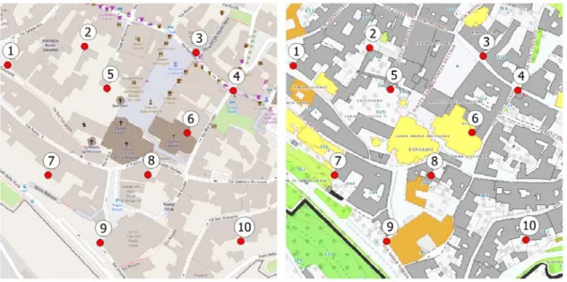
Referring to the semantic aspect and focusing only on the building footprints, the check can be easily done by extracting the layers corresponding to buildings from the two geodatabases. In the case of OSM, the features tagged as buildings are taken into account; in the case of the authoritative geodatabases, it depends on the conceptual schema and the adopted nomenclature. In the following, we assume that this step has already been carried out and we refer to the description of the case study presented in the next session for further details. Figure1shows an example of some homologous points that can be manually detected in the same area of two different maps.

ISPRS Int. J. Geo-Inf.2018,7, 289 8 of 25 ISPRS Int. J. Geo‐Inf. 2018, 7, x FOR PEER REVIEW   8 of 24

Figure 1. Example of homologous points on two different maps.

Before starting the detecting operation, we perform a raw fitting of the two maps, consisting in  an affine transformation, done by applying a least square estimate on (at least) five visually and  manually selected points. In the case of a rectangular map, the best choice is to pick out four points  at the corners and the fifth in the center of the map. 

The affine transformation is widely applied in map conflation, especially when the coordinate  systems of one or both of the datasets are unknown. In most cases, the coordinate systems of the maps  are known and it should be possible to directly overlap the two datasets without a pre‐alignment.  Even if the affine transformation cannot decrease local deformations by applying the same geometric  correction homogeneously over the entire dataset, it is always preliminarily applied by the algorithm  in order to reduce any systematic misalignments eventually introduced by approximate geodetic  transformation methods often used in the common Geographic Information System (GIS). Moreover,  the pre‐transformation allows the users to indistinctly apply the algorithm independently of the  known or unknown coordinate reference systems, thus making it a generalized approach. 

The algorithm allows the user to choose the type of affine transformation depending on the type  of cartographic data taken into account: 

‐ The general affine transformation, consisting of a roto‐translation with anisotropic variation of  scale and skew (six parameters), can be used when there is no information on the reference  system of the map to be evaluated and/or the acquisition methods (e.g., digitization of scanned  paper maps) may have been homogeneously distorted the map altering the corners (e.g., altering  the scale only along the acquisition axis of the scanner); 

‐ The conform transformation, consisting of a roto‐translation with isotropic variation of scale  (four parameters), can be used when you want to be sure that the transformation does not  change the shape of the geometries (preserving the corners of the original map); 

‐ The translation, consisting of a degeneration of the affine transformation in which only the two  shifts along the Cartesian axes are estimated (two parameters), can be used when the two maps  are not in the same reference system but these are known: it is therefore possible to apply a  datum transformation, usually implemented by the most common GIS. In these cases, the  translation can compensate for any slight misalignments due to the fact that in some cases these  transformation formulas are not rigorous but derived from approximate estimates. 

Finally, it is also possible to avoid the pre‐alignment of the two maps when they are natively in  the same reference system or the user is certain that the transformation between datums has been  carried out with rigorous methods. 

Depending on the choice of applying the affine transformation or not, the algorithm searches the  homologous points in an iterative process or in one step. 

Figure 1.Example of homologous points on two different maps.

Before starting the detecting operation, we perform a raw fitting of the two maps, consisting in an affine transformation, done by applying a least square estimate on (at least) five visually and manually selected points. In the case of a rectangular map, the best choice is to pick out four points at the corners and the fifth in the center of the map.

The affine transformation is widely applied in map conflation, especially when the coordinate systems of one or both of the datasets are unknown. In most cases, the coordinate systems of the maps are known and it should be possible to directly overlap the two datasets without a pre-alignment. Even if the affine transformation cannot decrease local deformations by applying the same geometric correction homogeneously over the entire dataset, it is always preliminarily applied by the algorithm in order to reduce any systematic misalignments eventually introduced by approximate geodetic transformation methods often used in the common Geographic Information System (GIS). Moreover, the pre-transformation allows the users to indistinctly apply the algorithm independently of the known or unknown coordinate reference systems, thus making it a generalized approach.

The algorithm allows the user to choose the type of affine transformation depending on the type of cartographic data taken into account:

- The general affine transformation, consisting of a roto-translation with anisotropic variation of scale and skew (six parameters), can be used when there is no information on the reference system of the map to be evaluated and/or the acquisition methods (e.g., digitization of scanned paper maps) may have been homogeneously distorted the map altering the corners (e.g., altering the scale only along the acquisition axis of the scanner);

- The conform transformation, consisting of a roto-translation with isotropic variation of scale (four parameters), can be used when you want to be sure that the transformation does not change the shape of the geometries (preserving the corners of the original map);

- The translation, consisting of a degeneration of the affine transformation in which only the two shifts along the Cartesian axes are estimated (two parameters), can be used when the two maps are not in the same reference system but these are known: it is therefore possible to apply a datum transformation, usually implemented by the most common GIS. In these cases, the translation can compensate for any slight misalignments due to the fact that in some cases these transformation formulas are not rigorous but derived from approximate estimates.

Finally, it is also possible to avoid the pre-alignment of the two maps when they are natively in the same reference system or the user is certain that the transformation between datums has been carried out with rigorous methods.

Depending on the choice of applying the affine transformation or not, the algorithm searches the homologous points in an iterative process or in one step.

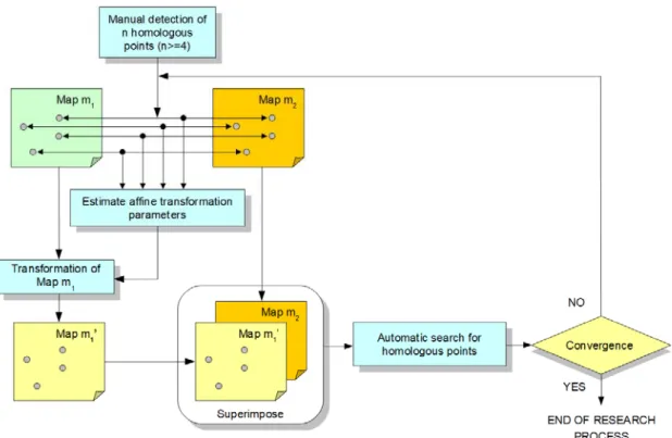
When the affine transformation is used, starting from the five points manually selected by the user, an iterative process is executed where at each step the affine parameters are estimated and the set of homologous points are determined. The whole procedure is repeated until the number of detected points becomes stable (see Figure2).

ISPRS Int. J. Geo‐Inf. 2018, 7, x FOR PEER REVIEW   9 of 24

When the transformation is not used, the set of homologous points are determined directly on  the original maps and the schema of the algorithm represented in Figure 2 is reduced to the process  box labeled with “Automatic search for homologous points”. 

Figure 2. Homologous points detection algorithm. 

The “Automatic search for homologous points” algorithm can be summarized as follows: if  dist(P1(i),P2(k)) is the distance from the point P1(i) on map m1 to point P2(k) on map m2, for each P1(i) 

(i = 1, …, N) on m1 we search for the point P2(k) on m2 which satisfies the condition of minimum 

distance from P1(i). If P1(i) and P2(k) are “geometrically compatible” (as described in detail below), 

P1(i) and P2(k) are set as homologous points. 

The algorithm allows the choice of two different distances to measure the proximity of the  candidate homologous points: a geometric distance and a statistic one. The former is the standard  Euclidean distance while the latter is based on a Fisher test to establish if two candidate homologous  points are compatible with the transformation model [34]. 

From the coordinates of the candidate homologous points and from the deterministic and  stochastic model of the least squares approach used to estimate the transformation, we compute a  variate F0, which can be compared, with a fixed significance level α, with the critical value Fα of a 

Fisher distribution of (2, n − m) degrees of freedom. The first degree of freedom (the value 2) expresses  the fact that we are considering a bi‐dimensional problem. In the second degree of freedom, the  number of observations used in the least square estimate—i.e., the n coordinates of the n/2  homologous points, and the m transformation parameters (6, 4, or 2, according to the chosen  transformation) appear. 

The test to accept the hypothesis H0: {P1 is homologous of P2} can be formulated as follow: if H0 

is true then F0 must be smaller than Fα with probability (1 − α), otherwise H0 is false.  Figure 2.Homologous points detection algorithm.

When the transformation is not used, the set of homologous points are determined directly on the original maps and the schema of the algorithm represented in Figure2is reduced to the process box labeled with “Automatic search for homologous points”.

The “Automatic search for homologous points” algorithm can be summarized as follows: if dist(P1(i),P2(k)) is the distance from the point P1(i) on map m1to point P2(k) on map m2, for each P1(i)

(i = 1, . . . , N) on m1we search for the point P2(k) on m2which satisfies the condition of minimum

distance from P1(i). If P1(i) and P2(k) are “geometrically compatible” (as described in detail below),

P1(i) and P2(k) are set as homologous points.

The algorithm allows the choice of two different distances to measure the proximity of the candidate homologous points: a geometric distance and a statistic one. The former is the standard Euclidean distance while the latter is based on a Fisher test to establish if two candidate homologous points are compatible with the transformation model [34].

From the coordinates of the candidate homologous points and from the deterministic and stochastic model of the least squares approach used to estimate the transformation, we compute a variate F0, which can be compared, with a fixed significance levelα, with the critical value Fαof a

Fisher distribution of (2, n−m) degrees of freedom. The first degree of freedom (the value 2) expresses the fact that we are considering a bi-dimensional problem. In the second degree of freedom, the number

ISPRS Int. J. Geo-Inf.2018,7, 289 10 of 25

of observations used in the least square estimate—i.e., the n coordinates of the n/2 homologous points, and the m transformation parameters (6, 4, or 2, according to the chosen transformation) appear.

The test to accept the hypothesis H0: {P1is homologous of P2} can be formulated as follow: if H0

is true then F0must be smaller than Fαwith probability (1−α), otherwise H0is false.

Without detailing the test, we notice that moreover, to guarantee the uniqueness of the associations, for each point P1(i) on m1and the N points P2(k) (k = 1, . . . , N) on m2which satisfy the hypothesis H0,

we selected the pair with smallest F0.

The advantage of this approach, compared with the simple check of the standard geometric distance, is having a probability index that expresses the precision and the correctness of each homologous point association.

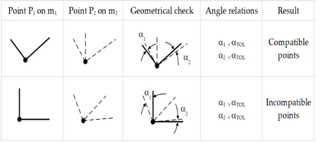
Beyond the distance, the “geometric compatibility” is based on the direction angles of the segments starting from the points and the inner corner of the edges of the polygon measured along the perimeter in a clockwise orientation.

Two points have an angle compatibility if both the direction angles of the common incoming segments and the corner angles are similar within a certain tolerance, hereafter indicated asα_TOL(see Figure3).

ISPRS Int. J. Geo‐Inf. 2018, 7, x FOR PEER REVIEW   10 of 24

hypothesis H0, we selected the pair with smallest F0. 

The advantage of this approach, compared with the simple check of the standard geometric  distance, is having a probability index that expresses the precision and the correctness of each  homologous point association. 

Beyond the distance, the “geometric compatibility” is based on the direction angles of the  segments starting from the points and the inner corner of the edges of the polygon measured along  the perimeter in a clockwise orientation. 

Two points have an angle compatibility if both the direction angles of the common incoming  segments and the corner angles are similar within a certain tolerance, hereafter indicated as αTOL (see 

Figure 3). 

Figure 3. Examples of compatible/incompatible homologous points. 

A step‐by‐step description of the algorithm with the use of the affine transformation can be  summarized as follows: 

● manual selection of five homologous points on the two maps m1 and m2; 

● application of an affine transformation estimated using coordinates of the previous five points;  ● repeat 

● for each point P1 on the map m1: 

● search the point P2 on the map m2 which satisfies the following conditions:  ● minimum distance from P1 to P2 

● the direction angles of all the incoming segments from the point P1 are similar, within  a certain tolerance αTOL, to all the incoming segments from the point P2 

● the inner corner of the edges P1 measured along the perimeter of the polygon in a  clockwise orientation is similar, within a certain tolerance αTOL, to the inner corner of  the edges P2 

● if P2 exists, set P2 as the homologous point of P1 

● application of an affine transformation estimated using the new automatically detected  homologous points  

● until the count of homologous points converges 

A step‐by‐step description of the algorithm without the use of the affine transformation can be  summarized as follows: 

Figure 3.Examples of compatible/incompatible homologous points.

A step-by-step description of the algorithm with the use of the affine transformation can be summarized as follows:

• manual selection of five homologous points on the two maps m1and m2;

• application of an affine transformation estimated using coordinates of the previous five points;

• repeat

• for each point P1on the map m1:

• search the point P2on the map m2which satisfies the following conditions: • minimum distance from P1to P2

• the direction angles of all the incoming segments from the point P1are similar,

within a certain toleranceα_TOL, to all the incoming segments from the point P2 • the inner corner of the edges P1measured along the perimeter of the polygon in a

clockwise orientation is similar, within a certain toleranceα_TOL, to the inner corner of the edges P2

• application of an affine transformation estimated using the new automatically detected homologous points

• until the count of homologous points converges

A step-by-step description of the algorithm without the use of the affine transformation can be summarized as follows:

• for each point P1on the map m1:

• search the point P2on the map m2which satisfies the following conditions: • minimum distance from P1to P2

• the direction angles of all the incoming segments from the point P1are similar, within a

certain toleranceα_TOL, to all the incoming segments from the point P2

• the inner corner of the edges P1measured along the perimeter of the polygon in a

clockwise orientation is similar, within a certain toleranceα_TOL, to the inner corner of the edges P2

• if P2exists, set P2as the homologous point of P1

It is important to underline that the map transformation is used by the algorithm exclusively in the iterative search for the homologous pairs. The algorithm does not alter the coordinates of the input data and therefore the coordinates of the homologous points exactly match the coordinates of the original maps. In this way, the distance of the pairs can be used as a correct indicator for the assessment of the spatial accuracy of the maps.

A possible problem, also found in the test case shown in the next section, consists in not being able to find homologous points, in certain areas, due to the incompleteness of one or both maps. In fact, there may be situations in which in some areas there are data in the former map but not in the latter or vice versa. Generally, the reasons vary: maps may have been made or updated at different times and therefore what they depict is not exactly the same due to the evolution of the territory; they may depict different LoDs; or simply, and this is common enough in OpenStreetMap, some areas are less mapped because of a lack of volunteers in those zones who decided to map them.

Obviously, this is a factor that we have to consider in our analysis. As we are using an automatic detection of homologous pairs, some non-recognition of homologous points could be due to limitations inherent in the adopted method. Others, like the one mentioned, are unavoidable and even the most meticulous manual operator would not detect them.

4. Methodology: Completeness

For dealing with the incompleteness of the data, a parameter, distdata, was defined. This can

be calculated by comparing the number of detected points with the total number of vertices of all the buildings on the two maps (therefore we have two values, corresponding respectively to the former and latter map). Moreover, for dealing with the different levels of detail, to avoid considering missing buildings, a corrective calculation was introduced which does not consider the vertices of the buildings present in the first map that are not represented in the second one when counting the potential homologous pairs (i.e., the total number of vertices of the buildings).

Finally, we defined that a vertex on the first map does not have potential homologous in the second one (and must not be counted in the statistics) if there are no vertices in a significant neighborhood, where the significant neighborhood depends on the parameter distdata. These points are called “isolated

points”.

The reasoning used for the completeness of the points can easily be extended to calculate the completeness of buildings. In fact, if all the vertices of a building are classified as isolate, then the building itself is considered isolated.

ISPRS Int. J. Geo-Inf.2018,7, 289 12 of 25

The percentage of isolated buildings can therefore be used, in addition to the quality of the data, to identify incomplete areas of a map (with respect to a more updated one) since the main and basic information usually depicted in a base map corresponds to streets and buildings.

The other factor that we mentioned and that has to be considered is the possible different levels of detail used to represent the same building on the two maps. According to the nominal scale of the maps (if this element was taken into account in its production; this is generally true for the authoritative maps) and to the different attention of the operators who digitized them, a building can be schematized for instance as a simple rectangle in a map or as a complex detailed polygon in the other one.

In this case, the more detailed map will have more points, many of which will not have a corresponding counterpart on the other map. These points, which we decided to call redundant points”, should not be considered when counting potential homologous pairs, similarly to what we did for the isolated points.

Another set of points we did not consider is composed of all the vertices that do not represent significant variations in the shape of the buildings. These points are essentially intermediate vertices positioned along the effective edges and describe the geometry of not perfectly straight lines or that are used to model non-accentuated curves as a succession of segments with slight angular variations.

Also, in this case, the positioning and the number of these vertices depend on the subjectivity of the digitizer and on the scale of representation of the map: therefore, it is advisable not to take them into consideration. The parameterα_tol, already defined to compute the angular compatibility of the vertices, can be used to set the threshold under which not to consider an edge significant and therefore disregard it in the search algorithm.

5. The Lombardy Region Case Study 5.1. The Regional Topographical Database (DBT)

The methodology discussed in the previous section was applied to Lombardy, which is one of the northern regions of Italy, with an extent of about 23,900 km2, a population of about 10 million and a population density of 420 people per km2. This area was chosen because of its high level of urbanization and because of the availability of a good authoritative map to be used for checking the quality of the OpenStreetMap data. The official vector base map of the Lombardy region is named Regional Topographical Database (DBT). The DBT is the digital reference base for all planning tools made both by local authorities and the region, as defined in article 3 of the Regional Law 12/2005 for the Government of the Territory. It is a geographic database comprising various digital territorial information layers that represent and describe the topographic objects of the territory. Its main contents are: buildings, roads, railways, bridges, viaducts, tunnels, natural and artificial watercourses, lakes, dams, hydraulic works, electricity networks, waterfalls, altimetric information (contour lines and elevation points), quarries and landfills, plant covers, etc. Each object consists of a cartographic feature and an alphanumeric table, to which any other descriptive information is added according to the thematic layer: use and state of conservation of the building (residential, industrial, commercial, etc.), type of road surface (asphalted, starred, composite pavement, etc.), type of vegetation (divided into forests, pastures, agricultural crops, urban green, areas without vegetation), etc.

The survey scale is very detailed for urban areas (1:1000–1:2000) and at medium-scale for extra-urban areas (1:5000–1:10,000).

The DBT is carried out in collaboration with local authorities to have a unitary and homogeneous cartographic reference for all municipalities, provinces, the Lombardy region, other authorities and professionals. It is the main cartographic data used to build a regional Territorial Information System (SIT) in which all the thematic data and the plans of the various authorities converge. The DBT is the appropriate basis for municipal urban planning and other land planning tools. Moreover, it is the reference for all cartographic elaborations for anyone who wants to present a project to a public administration.

The technical specifications of the DBT are defined in official documents where the geometric accuracy is also prescribed. The standard deviationσused as reference to define the accuracy of the map is defined for each cartographic scale. The tolerance for each DBT scale is defined equal to 2σ. The distribution of the residuals (the difference between the coordinate of the points stored in the DBT and their real coordinates, measured on randomly extracted samples) is always considered a normal one and therefore, in the quality control phase, only 5% of the absolute values of the differences can be higher than the tolerances. To further guarantee the quality of the data, the technical specifications prescribe that the residuals must in no case exceed twice this value; the maximum acceptable difference, in an absolute value, is therefore equal to 4σ.

Regarding the planimetric content of the DBT, the standard deviation for the various scales is as follows: for the scale 1:1000σ= 0.30 m; for the scale 1:2000σ= 0.60 m; for the scale 1:5000σ= 1.50 m; and for the scale 1:10,000σ= 3.00 m.

Similarly to the planimetric content, the altimetric accuracy is also prescribed. The standard deviation for the various scales is as follows: for the scale 1: 1000σ= 0.30 m; for the scale 1:2000

σ= 0.40 m; for the scale 1:5000σ= 1.00 m; and for the scale 1: 10,000σ= 2.00 m.

Since, in the OSM, the altimetric information is not defined for buildings, in our tests the altimetric quality was assessed.

5.2. Zonal Positional Accuracies

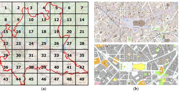
The whole area of the Lombardy region was considered for the comparison of the OSM buildings with the homologous DBT building layer and, in the first instance, the whole area was divided into squares using a regular grid of 7×7 cells (see Figure4). Splitting the region into cells was a result of the very large amount of data to be analyzed (as an order of magnitude, millions of buildings are involved). It is a common solution of breaking down a problem into more sub-problems of the same type, until these become simple enough to be directly solved [66]. The selection of the cell size was made based on two aspects: the type of possible misalignment of the two maps and the available hardware resources. When maps have a homogeneous misalignment, the cells can be wider than in the case of different localized misalignments, where a limited number of cells is preferred since the affine transformation is able to locally compensate for these deformations. Regarding the hardware resources, with smaller cells the computational performance is better (both in terms of required computation time and memory). A preliminary analysis of a sample dataset was performed and the optimal size of the cell was set to about 1000 km2. Considering the total area of the case study, the minimum cell number of a regular grid that contains the whole region is equal to 49 (7×7). The irregular shape of the region leaves 11 cells without data. Hence the following results will refer to a sub-dataset of 38 cells instead of 49.

Since both the DBT and the OSM are dynamic maps constantly updated in a non-homogeneous way, it is not possible to define a unique date of realization of the whole dataset. It is therefore difficult to have a time alignment of the two maps since it would be necessary to compare the update dates zone by zone. Anyhow, in order to have a “time stamp” of the data used in the following tests, both maps were downloaded from the official repository at the same time (August 2017).

The parameters for the homologous points search algorithm were set according to the DBT accuracy. The maximum distance within which to search for a homologous point was set to 4σ, corresponding to the maximum acceptable tolerance of the DBT.

ISPRS Int. J. Geo-Inf.2018,7, 289 14 of 25 ISPRS Int. J. Geo‐Inf. 2018, 7, x FOR PEER REVIEW   13 of 24

Regarding the planimetric content of the DBT, the standard deviation for the various scales is as  follows: for the scale 1:1000 σ = 0.30 m; for the scale 1:2000 σ = 0.60 m; for the scale 1:5000 σ = 1.50 m;  and for the scale 1:10,000 σ = 3.00 m. 

Similarly to the planimetric content, the altimetric accuracy is also prescribed. The standard  deviation for the various scales is as follows: for the scale 1: 1000 σ = 0.30 m; for the scale 1:2000 σ =  0.40 m; for the scale 1:5000 σ = 1.00 m; and for the scale 1: 10,000 σ = 2.00 m. 

Since, in the OSM, the altimetric information is not defined for buildings, in our tests the  altimetric quality was assessed. 

5.2. Zonal Positional Accuracies 

The whole area of the Lombardy region was considered for the comparison of the OSM buildings  with the homologous DBT building layer and, in the first instance, the whole area was divided into  squares using a regular grid of 7 × 7 cells (see Figure 4). Splitting the region into cells was a result of  the very large amount of data to be analyzed (as an order of magnitude, millions of buildings are  involved). It is a common solution of breaking down a problem into more sub‐problems of the same  type, until these become simple enough to be directly solved [66]. The selection of the cell size was  made based on two aspects: the type of possible misalignment of the two maps and the available  hardware resources. When maps have a homogeneous misalignment, the cells can be wider than in  the case of different localized misalignments, where a limited number of cells is preferred since the  affine transformation is able to locally compensate for these deformations. Regarding the hardware  resources, with smaller cells the computational performance is better (both in terms of required  computation time and memory). A preliminary analysis of a sample dataset was performed and the  optimal size of the cell was set to about 1000 km2_{. Considering the total area of the case study, the} 

minimum cell number of a regular grid that contains the whole region is equal to 49 (7 × 7). The  irregular shape of the region leaves 11 cells without data. Hence the following results will refer to a  sub‐dataset of 38 cells instead of 49. 

(a)  (b) 

Figure 4. (a) The regular grid used to analyze the Lombardy region delimited by red line; (b) one  example of the OSM map (up) and the DBT map (bottom) of the same place. 

Since both the DBT and the OSM are dynamic maps constantly updated in a non‐homogeneous  way, it is not possible to define a unique date of realization of the whole dataset. It is therefore difficult  to have a time alignment of the two maps since it would be necessary to compare the update dates  zone by zone. Anyhow, in order to have a “time stamp” of the data used in the following tests, both  maps were downloaded from the official repository at the same time (August 2017). 

Figure 4. (a) The regular grid used to analyze the Lombardy region delimited by red line; (b) one example of the OSM map (up) and the DBT map (bottom) of the same place.

Since the DBT Lombardy region is a mosaic of different local DBT at different scales (usually 1:1000 for historical centers of the city, 1:2000 for dense urbanized area, 1:5000 for peripheral sparse urbanized area and 1:10,000 for non-urbanized areas), the least restrictive tolerance among the urbanized areas was considered (σ= 1.50 m). The maximum distance was therefore set to 6.0 m.

Based on the same reasoning, the maximum distance used to consider a building to be isolated (isolated = without a corresponding homologous building on the other map), was set to twice the maximum tolerance and therefore set to 12.0 m.

Since only buildings were taken into account as geometric entities, the edges can define the shapes usually have corners of about 90 degrees and, more generally, greater than 45 degrees. With such a wide margin, it is therefore reasonable to not consider any data with vertices corresponding to angles of less than 10 degrees.

In the DBT, the building is defined as the whole of the volumetric unit that forms a body with a single building type; it may have several categories of use, it has a given state of conservation and it may have underground portions. Several alphanumeric attributes are available to describe it in detail. The main data are the building type (attribute: EDIFC_TY; values: generic house, terraced house, sports building, skyscraper, shed, monumental building, castle, etc.), the use (attribute EDIFC_USO; values: administrative, residential, public service, transportation services, commercial, industrial, etc.), and the state of conservation (attribute: EDIFC_STAT; values: in use, under construction, disused, etc.). In order to make a direct comparison with the OSM buildings, only the geometries of the DBT buildings are taken into account, i.e., those being compatible with the OSM building model.

OpenStreetMap features are provided according to a topological data model [67]. The nodes describe points in the space by their latitude, longitude, and their identifier. The ways, which describe links, consisting of an identifier and an ordered list of between 2 and 2000 nodes. Relations allow the description of relationships between elements (which can be nodes, ways, and other relations). A feature is based on one of those three elements. Furthermore, it consists of a list of pairs (a key and a value) of called tags. Even if in principle arbitrary keys and values can be added to features, the OSM community agrees on certain key-value combinations for the most commonly used tags.

In the “standard” OSM model, buildings are features that have a tag with the key “building” [67]. The value of the tag may describe the type of accommodation (e.g., “apartments”), of commercial use (e.g., “warehouse”), of religious use (e.g., “cathedral”), or of civic/amenity use (e.g., “train station”),

even if the most basic one is simply: “building = yes”. For about 82% of all buildings [20], the value of the tag is purely “yes”. For our purpose, we considered all typologies. There are currently about 282 million buildings in the OSM dataset [67], about 940 thousand in the Lombardy region. These buildings were used in our checking, subdividing them according to the grid we used for the DBT.

As explained in the previous theoretical section, the algorithm allows us to choose whether to apply a pre-alignment of the maps with an affine transformation (using an iterative approach) or to proceed directly to the search of the homologous points in one step.

In the following tests, all the solutions were investigated in order to analyze the differences, both in terms of homologous points found and in terms of reported statistical accuracy.

We expect that as a result of increasing the number of parameters of the transformation from 0 parameters (no transformation) up to six parameters (general affine transformation), the alignment of the two maps improves and therefore the number of homologous points, detected by the algorithm, increases. The greater the initial misalignment of the two maps, the greater the increase will be. Conversely, if the two maps are already well aligned, the number of homologous points is stable when the transformation changes.

Regardless of the number of points, if the accuracy of the OSM map is substantially homogeneous on the examined territory, the statistics on the distance between the homologous pairs should not change significantly. In fact it is important to remember that the transformation of the map is used exclusively in the iterative search process of the homologous pairs. At the end of the process the statistics on the distance of the pairs are calculated on the coordinates of the original maps (otherwise the results would no longer represent the accuracy of the original OSM map but the accuracy of the geometrically altered OSM).

The results for each cell obtained with no transformation in the search process are shown in Figure5, while the results obtained using the general affine transformation in the search process are shown in Figure6. Specifically, for each cell in Figures5a and6a, the number and percentage of homologous points detected by the algorithm are reported, while Figures5b and6b show the mean (M) and the standard deviation (S) of the distance of the points in the two maps. To get an indication of the correction to the statistics due to the highest number of homologous points detected using the affine transformation, the average differences are about 0.02 m for the mean and 0.03 m for the standard deviation. The results confirm that, in our case, the two datasets were already aligned since the pre-alignment does not introduce significant improvements on the number of points detected. We know that this is not true in general; for instance, in case of Munich an offset of about four meters on average in terms of positional accuracy was found [31]. Anyhow, the purpose of the proposed method was to be general and to allow global transformation for alleviating possible misalignments, which makes the automatic search of homologous pairs more difficult.

The percentages of homologous points detected with respect to the total potentially usable points (below indicated with P) can theoretically be computed both in the OSM map (POSM) and in the DBT

map (PDBT). By calculating these two values, it emerged that POSMwas always significantly greater

than PDBTand it can be explained taking into consideration the redundant points. In the OSM map,

the buildings are less detailed than in the DBT map and therefore there are more vertices in the DBT map that do not have a corresponding point in the OSM map. These points cannot be used by the algorithm and the result of the ratio between the number of homologous points detected and the total number of the points in the map inevitably decreases.