"Gimme Shelter" - A Long- and Short-Run Analysis of Swedish Regional House Prices

(1)

Master Thesis, Spring 2009 School of Economics and Management Lund University

“Gimme Shelter”

A Long- and Short-Run Analysis of Swedish Regional

House Prices

Authors: Sofia Bill Malin Ivarsson Supervisors: Klas Fregert Fredrik NG Andersson

(2)

“An economist is a man who states the obvious in terms of the incomprehensible.”

(3)

Abstract

The aim of this thesis is to examine the long-run relationship between regional house prices, how the house price model behaves in the short run and if aggregated national house price models may be misleading. To investigate whether house prices are related in the long run we use cointegration tests to look for common trends. The short-run behaviour of the model is estimated by an error correction model. To test the hypothesis that aggregated models are misleading, we compare the regional models and also use the same procedure to estimate the house price model with panel data. The results show that there are several long-run relationships between house prices of different regions. In the short run, CPI seems to have an important impact on house price changes in all regions whereas GDP and unemployment mainly influences house price movements in the metropolitan areas and the southern half of Sweden. The results from the panel regression lead to similar conclusions regarding the independent variables. Although the results are similar regarding the statistical significance of the variables, we cannot say anything regarding differences in economic significance between regions when using panel data and an aggregated model may thus be misleading.

(4)

List of Figures and Tables

Figure 4.1 House Price Index: All Regions (1981=100) Figure 4.2 Consumer Price Index (1980=100)

Figure 4.3 Real GDP

Figure 4.4 Short-Term and Long-Term Interest Rates Figure 4.4 Unemployment

Figure 5.1 House Price Ratios to National Average

Table 4.1 Definitions of Regions

Table 5.1 Results from group unit root tests on regional house price indices. Table 5.2 Results from cointegration test on all regional house price indices. Table 5.3 Results from cointegration testing of regions in Northern Sweden Table 5.4 Results from cointegration testing of regions in Middle Sweden

Table 5.5 Results from cointegration testing of regions in South-West of Sweden Table 5.6 Results from cointegration testing in metropolitan areas

Table 5.7 Results from cointegration testing between regions and the national average Table 6.1 Unit root test results, national variables

Table 6.2 Unit root test results, regional variables Table 6.3 Unit root test results, residuals

Table 6.4 Estimation output from the ECM of selected regions

Table 6.5 Panel unit root tests of the variables included in the house price model Table 6.6 Results from Pedroni panel cointegration test

Table 6.7 Results from Kao panel cointegration test

Table 6.8 Results from combined Johansen panel cointegration test Table 6.9 Panel unit root test results, residuals

(6)

1 Introduction

This chapter aims to introduce the purpose of the thesis and its delimitations. A short summary of the employed methodology and the results is also included together with a description of the outline of the thesis.

1.1 Aim and Purpose

The current state of the world economy once again confirms how important the role of the housing market is. Changes in the housing finance systems over the past decades have often lead to easier access on the mortgage markets, enabling even less suitable borrowers to finance a home ownership and increase their consumption. These so called subprime loans have made a large contribution to the crisis in the US of today. Rising house prices allow homeowners to increase their household borrowing, using their home as collateral. In due time the price bubble is bound to burst and some borrowers suddenly face negative equity, i.e. the cost of the mortgage exceeds the value of the house used as collateral. Another interesting macroeconomic aspect of the housing market is that housing wealth forms a large part of private wealth and that house prices therefore may have a large impact on the household’s consumption and saving behaviour. This is why studies of the housing market’s interconnections with the macro economy are so frequent and in demand by policy makers. Local factors play an important role in determining supply and demand on the housing market which induces substantial regional differences.

The purpose of this thesis is to model regional house prices in Sweden and to look for long-run relationships in, firstly, a panel of the house price indices of eight different regions and regions divided into smaller groups. Secondly the different regional macroeconomic variables that form the house price model are tested for long-run relationships and thirdly the same tests are performed on a panel of macroeconomic variables. The housing price model can then be estimated using both regional error correction models (ECM) and a panel ECM. Our contribution to the already existing studies is the panel cointegration approach with the use of regional data instead of aggregated data on the national level.

The questions to be answered are: Is there a long-run relationship between regional house prices and are there long-run relationships between house prices in different groupings of

(7)

regions? How do the components of the house price model behave in the short run and how does it respond to periods of disequilibrium?

1.3 Delimitations

To increase the number of observations, quarterly data is employed. This in turn imposes some restrictions on the availability of especially regional data. Whereas the interest rate is the same for all regions, measures of regional disposable income or GRP (gross regional product) are only available as yearly observations. Production levels are therefore measured by the aggregated GDP which naturally becomes the same for all regions. The lack of quarterly data leads to the only regional specific variables being house prices and unemployment, where unemployment is used as an indicator of regional production and uncertainty. Sweden is divided into eight regions (riksområden) which is a common used classification.

1.4 Disposition

The thesis is divided into three parts, where the first part is a cointegration analysis of the regional house price data. The aim of the first part is to investigate if there is a long-run common trend between the different regions’ house prices. The second part investigates how the different variables affect the house prices in the different regions. Do the regions react differently and do they have differences in their speed of adjustment. Regional data is used as aggregated house prices models may overlook important regional factors and differences. The final part performs an ECM on panel data, testing for which variables that affect the house prices.

The first chapter is an introduction to the thesis that states its aim and purpose. The second chapter depicts the background of the thesis and investigates previous research. The model used is presented in chapter 3 along with the theory and the methodology. The fourth chapter describes the data. In chapter 5 and 6 the results are presented, followed by a discussion in chapter 7. The last chapter is a conclusion of the thesis.

(8)

2 Background and Previous Research

This section presents essential information to understand the importance of investigating the housing market and the contemporaneity of the subject together with part of the research previously conducted. The chapter also includes our hypothesis about regional housing markets.

2.1 Background

The housing market plays an important role in the economy and the importance keeps increasing. Over the last two decades the housing financing system has experienced a lot of innovation and changes. The dynamics of the housing sector depends a lot on the local factors, which determine the supply and demand, and the structure of the mortgage market. The Swedish housing financial market experienced a deregulation in the mid 1980’s (IMF, 2008) and the housing market experienced a price boom in the late eighties, where the prices first increased substantially and then decreased by about the same amount some years later (ECB, 2000). A tax reform (91TR) was implemented in Sweden in 1991 with one of the aims being to decrease the distortion on the housing market. The tax reform meant that the deduction of interest payments was decreased, which resulted in higher user cost for private home owners (Barot & Yang, 2002). In recent years both the mortgage debts and the role of houses as collateral in Sweden have increased (Statistics Sweden, 2009). The mortgage market has experienced increased competiveness and flexibility which has made the Swedish mortgage market one of the most flexible and “complete” with easy access to mortgage credit.

These changes have led to increased spill-over effects from the housing market to the rest of the economy mainly due to the positive effect on consumption via increased household debt leverage (IMF, 2008). When houses are used as collaterals, an increase in house prices also increases the value of the collateral, which in turns leads to an increased consumption. When combining this with an expectation of higher future income, the effect gets extra strong as it allows the households to borrow against a higher expected income. Due to all these changes the role of the house sector on business cycles have also altered and become increasingly important. This has also led to an increased effect of monetary policy on house prices and thereby on consumption and output. The house prices have had a tendency to be closely correlated with the economic cycle, but with a lag of six quarters for Sweden (IMF, 2008). The increased role of the housing sector was for instance showed by the enlarged contribution to the downturn of GDP by the residential investment compared to previous decades. The

(9)

modification of the housing financing system has also led to an increased sensitivity and exposure to shocks from the housing sector. It is not only the role of the housing sector that has changed, the housing cycles have also altered their appearance by lasting longer and being stronger.

As mentioned the house prices have an increasingly important effect on consumption. The previous research on the Swedish housing market mainly investigates how the housing market reacts to different shocks and how that in terms may affect the consumption. ECB (2000) conducted a study on which the main factors of fluctuations in the house prices are and concluded that monetary policy shocks have a great impact on house prices. House prices where also found to be more sensitive to changes in expectations than consumer prices are.

Housing markets have many special features resulting in that the structure of the housing market in some senses best is described as a collection of a lot of smaller regional markets. Cointegration studies between different regions have mainly been performed in Britain, where the researchers have tested for long-run relationships in house price changes between different regions on time series data, the so called “ripple effect” or “ripple down effect”. The “ripple effect” implies that house prices in one region are pulled up by the increase in house prices in some other region, the prominent region, and then pulled down by the decrease in prices in the same other region (MacDonald and Taylor 1993). In Britain the south-east region is said to be the prominent region of the ripple effect. As the ratio between the price in one region to the price of the prominent region is stationary it displays no long-run trend (Meen, 1999).

These studies can be implemented on the Swedish housing market in an interesting way. As shown by Barot and Yang (2002), there are many similarities between the housing markets in the two countries. In the British cointegration studies augmented Dickey Fuller tests (ADF test) are used to conclude whether there is any upward or downward trend in the series. The ADF tests search for unit roots and thereby tests for stationarity. If some stationary linear combination is found, the series are cointegrated. If house prices are non stationary and not cointegrated in two regions, the difference in house prices between the two regions will not return to an equilibrium level, it will increase over time, so there is no long-run stable pattern in the prices.

(10)

2.2 Previous Research

As mentioned in the background section a lot of the existing research on regional trends in the house prices has been performed in Britain due to the existence of the hypothesis of the “ripple effect”. MacDonald and Taylor (1993) analysed both the long-run and the short-run properties of regional house prices by testing for regional cointegration between house prices in Britain. The cointegration test showed that some interrelationships exist, indicating that there may be some segmentation of housing markets in Britain. When testing for the number of cointegrating vectors between the different regions, the Johansen maximum likelihood approach was used and up to nine cointegrating vectors was found, which increased the empirical support for earlier findings of a long-run interregional relationship in British residential house prices. In order to see how the different regions interact with each other, impulse response functions were computed and the results were in line with the “ripple effect”. As the “black box” technique was used, meaning that the regional interrelationships cannot be explained, the result cannot distinguish what caused the effect (MacDonald and Taylor, 1993). According to MacDonald and Taylor (1993) the result may have its cause either by arbitrage through house owners selling their houses in high price areas and moving to low price areas, or because there were some regional element to the business cycle in the data sample. MacDonald and Taylor can only conclude that there exists a “ripple effect”, not explain it.

Ashworth and Parker (1997) analysed the determinants of house prices in different regions in Britain by using the Johansen maximum likelihood (1991) technique, the same as MacDonald and Taylor (1993) but improved, on regional house price models. They investigate both the long-run structure of house prices and the short-run adjustments made by agents in the different regions. Ashworth and Parker used the equation derived by Drake1 which states that the private sector house price in period t is determined by household income, an opportunity cost variable, which is the real interest rate defined as the mortgage rate minus the house price inflation, and personal sector housing starts, all in the same time period. When using the Johansen maximum likelihood technique, the test showed that there was at least one cointegrating vector for all regions except two. The results for the vectors were all consistent with the predictions of the model, that income per capita had a positive effect on house prices and the opportunity cost and housing starts had negative effects.

1

The article that Ashworth and Parker (1997) refers to is ”Modelling UK House Prices Using Cointegration: An Application of the Johansen Technique” by Drake, L.M (1993)

(11)

Both substantial similarities and differences were found between the regions. When comparing the results for each region to the ones for the whole nation, the results were mixed. For the regions that have a prominent role in the British house market the difference was insignificant, as expected, but some other regions also experience insignificant results which could not be explained. Some differences were however found to be significant, indicating that the findings for the aggregated data on Britain could be misleading (Ashworth and Parker, 1997). For some regions the housing starts have a large impact on house prices while the effect is almost insignificant for other regions and the aggregated data shows that house starts are only significant at a ten per cent level. These differences support the earlier conclusions that when only looking at the aggregated data it may not consider the regional differences. There were considerable effects of the interest rate on house prices in the long run. Other variables that may affect the housing market in different ways regionally were changes in housing construction guidelines and changes in per capita income. Ashworth and Parker (1997) explain the lack of long-run relationships with the possibility of structural differences between the regions.

Ashworth and Parker (1997) use the Granger’s (1983) Representation Theorem, which states that a short-run error correction mechanism is included in every long-run cointegration relationship, to further investigate the housing markets. The error correction mechanism describes how agents in the different regions respond to short-run changes in the economic environment. The results showed that there is a substantial similarity between different regions in the agents’ short-run behaviour such as the negative effect of opportunity costs on house prices and positive secular growth. The test also showed that the adjustments conducted by the agents are in general small, suggesting that the return to equilibrium may be concealed by the short-run changes in economic conditions. According to Ashworth and Parker (1997) their results demonstrate some automatic correlations in the behaviour of the house prices. In all short-run analyses, housing starts are not included in the regressions as they were not found to be significant and as they are argued to have long-run supply effects. When comparing the short-run regional results with the aggregated, many similarities were found. Income had a positive effect on house prices, opportunity cost a negative and housing starts are not included in any of the short-run analyses. The error correction term had a low speed of adjustment, but that could be explained by the large cost of adjusting the house stock due to transaction and search costs. When performing spatial correlation tests, which show to what

(12)

extent regions are linked to each other, the results contradicted the “ripple effect” and showed that the adjustment appeared at the same time in all the regions. Ashworth and Parker (1997) speculate that the disappearance of the “ripple effect” is due to their assumptions considering economic theory.

Meen (1999) proposes a regional house price ratio model which captures not only income differences and spatial lags but also structural differences between the regions, by testing for coefficient differences. An equation is estimated were house prices are a function of nominal interest rate, real income, which is measured by consumers’ expenditures, unemployment rate, which is a measurement of risk, and an error term. An ADF test is used to test for the possible consistency of a long-run ratio and the results show that there may have been a weak trend in relative prices. House prices move proportionately in the long run and in common for all regions is that they are sensitive to income changes. Income changes are found to have a smaller negative effect on house prices in the northern regions than in the southern regions of Britain and the national average. The same holds for the interest rate which also has a smaller short-run effect in the north. According to Meen (1999) the south would be more sensitive to changes in interest rates as there is higher leverage in the south than in the north, which also should explain the higher speed of adjustment and their higher sensitivity to unemployment.

Meen (1999) argues that even though there may be some variations in the short run in the difference between the prices in different regions, in the long run the relative prices return to their normal state. This is also shown when Meen (1999) tests how the different regions react to shocks in the national variables. Meen (1999), as Ashworth and Parker (1997), concludes that when adding economic effects to the analysis of the “ripple effect”, the result is not definitive. This is in contrast to MacDonald and Taylor (1993) who argues for the existence of the “ripple effect”, but cannot conclude what the cause of it is. They claim that the effect arises due to arbitrage or some regional components to the business cycle in the data (MacDonald and Taylor, 1993). According to Meen (1999) Britain’s housing market is best described as a collection of regional markets, which all have some structural differences which in turn affect national housing market models. These possible structural differences are another motivation of why distinguishing between the regional markets, instead of just looking at the aggregated models, is important. In contrast to Ashworth and Parker (1997), Meen (1999) claims that the “ripple effect” does not only occur because of spatial correlation, but that the same effect can be obtained by coefficient heterogeneity. The heterogeneity

(13)

measures structural differences between regions such as differences in behaviour. Meen (1999) argues that changes in regional house prices can be decomposed into three smaller parts, common movements in all regions, movements due to different economic growth in different regions and structural differences in the regional markets. According to Meen (1999) there is spatial correlation between the coefficients causing changes in the housing market that we interpret as the “ripple effect”, when the true cause lies in the changes within the regions and not between different regions.

Hort (1998) investigates the determinants of urban real house price fluctuations in Sweden between the years 1968-1994. She estimated a restricted ECM of real house price changes on Swedish panel data. Changes in income, construction cost and user cost where found to affect the real house prices in the long run and also included a negative deterministic trend as a proxy for factors not included in the model. According to Hort, 80 % of the fluctuations in real house price changes can be explained by her short-run model and that periods of disequilibrium could explain the short-term prices.

Barot and Yang (2002) compare the Swedish and the British housing markets using an ECM by estimating housing demand and investment supply. They found that change in income, debt, real interest rate and Tobin’s Q affect the house prices in both Sweden and Britain, but that the change in debt affects the British house prices more than the Swedish and that the opposite holds for the interest rates. When testing for Granger causality, changes in financial wealth affected the house prices in Sweden. The house prices also have an impact on some of the variables in both countries, such as financial wealth, debt, real interest rate and Tobin’s Q in Sweden and on income, debt and real interest rate in Britain. When departing from the equilibrium level, twelve per cent of the shock is adjusted within a year in Sweden and twenty-three per cent in Britain. In both Sweden and Britain demographic changes are found to have strong effects on house prices (Barot and Yang, 2002).

2.3 Hypothesis

The authors regarded in the previous research section have proved that there are substantial regional differences in Britain. Whether these are a result of the “ripple effect” or structural differences between the regions may however be a subject for further discussion. As mentioned by Barot and Yang (2002) the house market in Britain and Sweden experience

(14)

some similarities in the regional differences in the countries’ house prices. We expect that the eight Swedish regions will be cointegrated with each other, i.e. that there is a long-run relationship between the house prices in the regions. This hypothesis will be tested in section 5.1.2.1. Between the regions that in some way resemble each other a long-run relationship in house prices is expected. The resemblance could be due to geographical proximity or the existence of metropolitan areas in the region. Which features that are most important for the resemblance in the markets are tested in section 5.1.2.2 and in 5.1.2.3. Of the eight different markets in Sweden we expect that the most northern region and the regions containing a metropolitan area would differ most from the average housing market, in section 5.1.2.4 a test of this hypothesis will be performed.

The national housing market is often best described as a collection of many small markets (Meen, 1999). We use the classification of the regions as the definition of the smaller markets that the national market consists of. These markets may be similar in some cases and diverge from each other in other cases. The short-run behaviour of the housing markets in the metropolitan areas could be expected to be different compared to the markets in regions without any special features such as a large city or a sparsely population. As Meen (1999) concluded, changes in the interest rate have smaller effects in the northern regions than in the south which could be a result of lower leverage in the northern regions. This would also make the northern regions less sensitive to other variables such as unemployment. One may suggest that the regions in Sweden may show a similar pattern. As prices are lower in the northern regions in Sweden than in the south and in the metropolitan areas, households in the northern regions borrow less and are thereby less sensitive to changes in interest rates and unemployment. A decrease in income would have a negative affect in all regions; the effect might be less negative in the northern regions than in the south and metropolitan areas. This hypothesis will be tested in section 6.1.3.

In general, our hypothesis is that there will be a difference between the regional housing markets and studies of the aggregated national market may thus be misleading, since it does not account for regional features of the housing markets.

(15)

3 Theory and Methodology

The aim of this section is mainly to explain the methods used to test our stated hypotheses. The econometric theory behind the performed tests and the model estimations is described in detail. Since our theory and methodology are converging, they are included in the same chapter.

3.1 Modelling House Prices

The existing work on the housing market is immense as well as the number of models trying to explain house prices. That some measure of income and interest rates should form the basis of the model is more or less agreed upon unanimously. Higher income affects demand and in turn has a positive effect on house prices, whereas higher interest rates raise the cost of borrowing and thus decrease the demand for housing which affect prices negatively. One question, of which the answer is not as obvious as with income and interest rates, is whether housing stock should be included or not when wanting to model the housing market. Looking to the theories of Sørensen and Whitta-Jacobsen (2005, pp. 454-455), housing stock only really matters in the short run. An increase in the housing stock with demand held constant will lower the price until, in the long run, demand has had time to adjust. Since we are interested in the long-run relationships of house prices and macro variables, we have decided to not take the housing stock into account on the basis of the arguments presented by Sørensen and Whitta-Jacobsen (2005).

The house price model in this thesis is inspired by the work of Meen (1999) described in chapter 2. His test of stationarity in the ratios between regional house prices corresponds to testing for cointegration. The model developed in his article explains house prices as a function of consumers’ expenditures, unemployment and nominal interest rates. Since the access to regional quarterly data is limited, we have substituted regional consumers’ expenditures by aggregate measures of GDP and instead use unemployment rates as an approximation of regional production fluctuations. Nominal interest rates have been specified as the short- and long-term interest rates (see data section for more details). The reason for including both the short- and the long-term interest rates is to examine if the different maturities might affect house prices in different ways. As opposed to Meen, we will examine house prices both regionally and in the form of panel data. The initial model on which we base our studies could be described as:

) , , , , ( _t _t _t _ts _tl H t f GDP CPI U r r p = (3.1)

(16)

where p_tH denotes the regional house price indices, GDP_t is the Swedish gross national product, CPIt denotes the consumer price index,Ut indicates regional unemployment and

s t

r and rtl are the short- and long term interest rates. All variables except the interest rates are logarithmized. The log-linear specification means that the slope coefficients generated from estimating the model should be interpreted as elasticities. The coefficients of the interest rates are semi-elasticities2.

To investigate the long-run relationships between regional house prices, we will perform a series of cointegration tests after having concluded that the variables are non-stationary through unit root testing. We will then move on to model the short-run behaviour of house prices by forming regional error correction models (ECM) with selected independent variables. This allows us to compare the short-run behaviour of house prices between regions. We will also estimate a panel ECM with the motivation that more observations may yield sharper results with increased efficiency. With panel data we will however not be able to draw any conclusions about possible differences between regions. The statistical programme used for testing and estimating the data is EViews version 6.

We will proceed as follows:

1) Testing for unit root in regional house prices and for cointegration between house prices in a panel consisting of eight regions and in smaller groupings.

2) Testing for unit root in the cross-sectional variables.

3) Testing for cointegration between the cross-sectional variables in the house price model defined in equation (3.1).

4) Estimating the regional house price models using an ECM.

5) Estimating the regional house price model with panel data using an ECM.

3.2 Theoretical Background to Methodology

3.2.1 Unit Root Testing

Since dealing with time series data always includes the risk of non-stationarity, it is important to consider this issue in order to not end up with spurious results. On the other hand, the

2

That interest rates are semi-elasticities means that an absolute change in interest rates leads to a percentage change in the dependent variable, i.e. house prices.

(17)

presence of a unit root (i.e. non-stationarity) and cointegration can be of economic interest. What is done when testing for a unit root is simply that it is tested if the coefficient of the lagged value of a variable equals one. Consider for example a simple AR(1) model:y_t =ρy_t₋₁+u_t. Taking first differences we get the Dickey-Fuller (DF) specification

t t

t y u

y = − +

Δ (ρ 1) ₋1 . The hypotheses to be tested will then be:

) 1 . . ( , 0 * : ) 1 . . ( , 0 ) 1 ( * : 1 0 < < = = − = ρ ρ ρ ρ ρ e i H e i H (3.2)

where the rejection of the null hypothesis indicates stationarity, i.e. no unit root. For the case of higher-order autoregressive models the DF-test is extended to an augmented DF-test (ADF test) where the auxiliary regression will look as follows:

∑

= − − + Δ + = Δ pi L t L t L t t y y u y 1 1 * ρ ρ (3.3)

Higher-order correlation is now controlled for by adding lags of the first differences of y_t. p_i

denotes the maximum number of lags chosen and the hypotheses to be tested are the same as for the simple DF test.3

An alternative test has been developed by Kwiatkowski, Phillips, Schmidt and Shin (KPSS) where the null hypothesis of stationarity is tested against the alternative of a unit root. Their idea was that time series are decomposed into sums of a deterministic trend, a random walk and a stationary error term and under the null the variance of the random walk component is zero. The test statistic used to test the hypotheses is a Lagrange multiplier (LM) statistic and besides which deterministic components to include, it must be specified which spectral estimation method to apply.4

3.2.2 Cointegration

Cointegration between two or more non-stationary variables means that there exists a linear combination of these variables that is stationary. The implication of cointegration is the occurrence of a long-run relationship between the included variables, which in many cases is suggested by economic theory. Hence the economic interest of testing for cointegration. Testing for cointegration can be done using the two-step Engle-Granger (EG) approach. Consider the simple model:

t t t x y =β +ε (3.4) 3

See for example Verbeek (2008) 4

(18)

and suppose that y_t and x_t are I(1) (i.e. non-stationary): y_t and x_t will be cointegrated if the residuals ε_t are I(0) (i.e. stationary). If the error term is stationary around zero it means that it is mean reverting and will occasionally equal zero so that yt =βxt in the long run. To test whether the residuals are stationary, the first step of the two-step EG approach is to estimate the simple model in equation (3.4) by ordinary least squares (OLS) and then save the estimated residuals and perform a unit root test on them by running the auxiliary ADF type regression:

∑

= − − + Δ + = Δ pi L t L t L t t u 1 1 * ˆ ˆ ˆ ρ ε ρ ε ε (3.5)

where p_i denotes the chosen lag length. If deterministic components like a constant or a trend are to be included, they should be added to one of the test equations (3.4) or (3.5) and never to both. In multivariate models with more than two endogenous variables, there exists the possibility of several cointegrating relationships and the EG single equation approach may in this case be misleading and an alternative way of testing for cointegration has therefore been developed by Johansen.5 This thesis will make use of both methods and since the Johansen procedure is rather complex, it will be explained in more detail below.

3.2.2.1 Cointegration Testing: The Johansen Approach

In the multivariate framework the possibility of more than one cointegrating relationship exists and an alternative approach to the Engle-Granger two-step procedure has been developed by Johansen who uses a maximum likelihood (ML) estimation method that allows the testing of the number of cointegrating relationships. Consider a vector autoregressive (VAR) specification with up to k lags of the vector z_t (a vector of n possibly endogenous variables): t k t k t t Az A z u z = ₁ ₋₁+...+ ₋ + (3.6) where zt is (n×1) and ut ~ IN(0,∑).

Equation (3.6) can be transformed into a vector error correction model (VECM) which is a VAR model that considers the common history of a number of endogenous variables, in error correction form: t k t k t k t t z z z u z =ΓΔ + +Γ Δ +Π + Δ 1 ₋1 ... ₋1 ₋ ₊1 ₋ (3.7) 5

(19)

If z_t is I(1), Δz_t is I(0) and this means that Πz_t₋_k must be I(0) for u_t to be white noise. This holds for three occasions: (i) when all variables in z_t are stationary, (ii) when there is no cointegration so that there are no long-run relationships between the variables in zt and (iii) the case of so called reduced rank when there are up to n−1 cointegration relationships r

and Π can be written as αβ′ where α is a speed of adjustment term and β is a matrix of long-run coefficients. The cases (i) and (ii) are of little interest in this context, since (i) implies that the problem of spurious results due to autocorrelation does not exist whereas (ii) requests that estimation is done employing a model that does not involve any long-run components, e.g. a VAR.

The presence of r≤(n−1) cointegrating relationships in β means that there are r columns that form r linear stationary combinations of the variables in the vector z_t and (n−r) columns that form non-stationary relationships. For Πz_t₋_k to remain stationary, only the cointegration vectors may enter equation (3.7) and this in turn implies that the last (n−r) columns in α are insignificant. Testing for cointegration thus means testing which columns in α that are zero or in other words how many rlinearly independent columns that can be found in Π. For a given r the ML estimate for β is the same as the eigenvectors corresponding to the r largest eigenvalues of a n×n matrix. The estimated eigenvalues

n

λ λ

λˆ ˆ _... ˆ

2

1 > > > can be used to test hypotheses about r (the rank of Π). If there are

rcointegration relationships, log(1−λˆi)=0 for the smallest (n−r) eigenvalues (i.e. for

n r r i = +1, +2,..., ): n r r H r r H ≤ < ≤ 0 1 0 0 : : (3.8) The null hypothesis is tested using the so-called trace statistic to see whether the smallest

)

(n−r0 eigenvalues are significantly different from zero:

∑

+ = − − = n r i i trace T 1 0 ) ˆ 1 log( λ λ (3.9)

Alternatively it can be tested whether the largest eigenvalue is significant using the maximum eigenvalue statistic: ) ˆ 1 log( 1 max =−T −λr₀+ λ (3.10)

(20)

where the null of r cointegration vectors is tested against the alternative of r+1 vectors. The tests are distributed under a multivariate DF distribution.6

3.2.3 Modelling Cointegrated Time Series

As mentioned in the beginning of section 3.2.1, estimating non-stationary time series may lead to spurious results. If this issue is not considered and one estimates a regression trying to explain y_t from x_t by OLS, one would probably end up with significant but misleading results. These so-called spurious regressions are characterized by high explanatory power (R2) and high t-statistics indicating significant values of the slope coefficients. The reason why the OLS estimator tends to indicate significant correlation between the variables even though they are uncorrelated is due to that they are both trending. If however the variables are cointegrated and share a common trend, consistent slope coefficients can be estimated by OLS and these estimated coefficients will even be super consistent, meaning that they converge towards their true value at a faster rate than usual OLS estimators. A spurious regression will have non-stationary error terms leading to inconsistent estimators of the slope coefficients. By testing the error terms as the EG approach prescribes one could conclude if OLS may be used to generate consistent estimators.7

A long-run cointegrating relationship suggests that conclusions can be drawn regarding the short-run adjustment behaviour of the non-stationary variables. If there exists a long-run relationshipy_t =βx_t, there must be some force that drives the equilibrium errorε_t = y_t −βx_t, i.e. the term that measures the distance away from equilibrium during periods of disequilibrium, back towards zero. This is modelled using an error correction model (ECM) where the equilibrium error is represented by the error correction term. The ECM could be said to be a continuation of the EG two-step procedure, since we need to affirm that the variables are cointegrated before we move on to estimating the model. Consider the simple model: t t t t t x x y u y =φ₀ +φ₁ ₋₁+α₁ ₋₁ + (3.11)

where φ₀ denotes the reaction of y_t to a change in x_t in the short run. Taking first differences gives:

6

See for example Harris and Sollis (2003) 7

(21)

t t t t t t t t t t t t t t t t t t t t t u x y x y u x y x y u y x x x y u y x x y + − − Δ = Δ ⇒ + ⎥ ⎦ ⎤ ⎢ ⎣ ⎡ ⎟⎟ ⎠ ⎞ ⎜⎜ ⎝ ⎛ − + − − − Δ = Δ + − − + + − = Δ + − + + = Δ − − − − − − − − − ) ( 1 ) 1 ( ) 1 ( ) ( ) ( ) 1 ( 1 1 0 1 1 1 0 1 1 0 1 1 1 1 0 1 0 1 1 1 1 0 β γ φ α φ φ α φ α φ φ φ α φ φ (3.12)

which represents the ECM where γ =(1−α₁) and _⎟⎟ ⎠ ⎞ ⎜⎜ ⎝ ⎛ − + = 1 1 0 1 α φ φ

β . If the error correction term

0 )

( 1 − 1 =

−γ yt₋ βxt₋ we are in equilibrium and the model becomes Δyt =φ0Δxt +ut. γ denotes the speed of adjustment towards equilibrium. Since it has already been concluded by the EG approach that we have cointegrated variables, equation (3.12) can be estimated by OLS despite the non-stationary properties of the data.8

3.3 Panel Data

The major advantage of working with panel data is the possibility to allow for heterogeneous individuals, in this case regions. In addition we get more variability and, since we combine cross-sectional observations we get a larger number of observations yielding more degrees of freedom, leading to greater efficiency when estimating the model.

A simple panel data model may look as follows: it it it

it X z e

y = ′β + ′γ + (3.13)

where i=1,...,N denotes individuals and t =1,...,T denotes time, X_it′ =

{

x₁_t,x₂_t,...,x_Nt

}

is a vector of N independent variables and z is a deterministic component which can take on several forms. Allowing for heterogeneity in individuals, i.e. to have separated intercepts, implies that z takes on the form of the fixed effect α_i. Another alternative would be to assume random effects which mean that αi is homoskedastic across individuals. This assumption is however more restrictive than the fixed effects.9

Applying this to our house price model inspired by Meen (1999)yit will denote H it

p and the vector X_it′ can be defined as:

{

l

}

it s it it it it it GDP CPI U r r X′ = , , , , (3.14) 8

(22)

Working with panel data also gives rise to some limitations. The assumption of independent observations will be hard to fulfil, since the same individuals are observed several times, which means that OLS estimators might be less efficient. This can however be resolved by using other estimates that take correlation of the error terms into account. When used correctly, panel data sets will actually often yield more accurate estimates than examinations of individual cross-sections.10

3.3.1 Panel Unit Root Testing

Although there are several advantages from working with panel data, additional issues arise when testing for unit roots in panels compared to the single time series case. Assumptions about cross-sectional independence have to be made, which contradicts the expectations of finding long-run relationships when testing for cointegration. It has been shown that many of the tests perform poorly when the error terms are sectionally correlated or under cross-sectional cointegration.11

There are several tests available for computing panel unit root tests and they can in turn be divided into two groups: tests with a common unit root process and tests with individual unit root processes.

3.3.1.1 Common Unit Root Process

Levin, Lin and Chu (2002) have developed a panel unit root test (LLC test) based on the ADF specification: it it p L L it iL it it y y z u y i + ′ + Δ + = Δ

∑

= − − ∗ _θ _γ ρ 1 1 (3.15)

where )ρ∗ =(ρ−1 is common for all cross-sections, but the lag order, p_i, for the differences is allowed to vary. The hypotheses to be tested are:

0 : 0 ) 1 ( : 1 0 < = − = ∗ ∗ ρ ρ ρ H H (3.16)

If the null hypothesis cannot be rejected all individuals contain a unit root and if the null can be rejected all individual series are stationary. Under the null the modified t-statistic for the estimated ρˆ , adjusted for serial correlation, is asymptotically normally distributed: ∗

10

See for example Verbeek (2008) 11

(23)

) 1 , 0 ( ) ˆ ( ˆ ) ~ ( ~ ~ 2 N se S T N t t T m T m N LLC → − = _∗ ∗ − ∗ σ μ ρ σ ρ (3.17)

where t_ρ∗ is the standard t-statistic for 0 : =0

∗

ρ

H , SN is the average standard deviation ratio, σˆ2 is the estimated variance of u_it, se(ρˆ)is the standard error of ρˆ, μ_m_T~∗ and ∗

T m~

σ

are adjustment terms for the mean and standard deviation and: 1 ~ _⎟₋ ⎠ ⎞ ⎜ ⎝ ⎛ − =

∑

i i N p T T (3.18)

Thus, inference can be performed using critical values based on the normal distribution as opposed to the first developed Levin, Lin (LL) test where new critical values adjusted for serial correlation had to be computed.

Another panel unit root test that accounts for a common unit root process is the Hadri test that is similar to the KPSS test described in short in 3.2.1. Unlike the LLC test, this test employs the null hypothesis of no unit root in any of the series against the alternative of a common unit root in the panel data. The test is based on the residuals generated from regressing yit on a constant or a constant and a trend and estimating the equation by OLS:

it i i

it t

y =δ +η +ε (3.19)

The estimated residuals εˆ are then used to form a Lagrange multiplier (LM) statistic that is _it standard normally distributed.12

3.3.1.2 Individual Unit Root Process

In common for the different tests in this category is that they all relax the homogeneity constraint imposed in the tests for a common unit root process by allowing for ρ to vary across the individual series. The Im, Pesaran and Shin (IPS) test is based on ADF specifications that are separate for each cross-section (as with the LLC test the lag length is allowed to vary between individuals):

it it p L L it iL it i it y y z u y i + ′ + Δ + = Δ

∑

= − − ∗ _θ _γ ρ 1 1 (3.20)

with the following hypotheses:

i one least at for H i H i i i 0 : 0 ) 1 ( : 1 0 < ∀ = − = ∗ ∗ ρ ρ ρ (3.21) 12

(24)

The null hypothesis, if not rejected, states that each series contains a unit root for all cross-sections against the alternative that at least one of the individual series is stationary. To get the

t-statistic, the IPS test averages the individual t-statistics obtained forρi∗and generates a standard normally distributed t-bar statistic:

∑

= ∗ = N i t N t 1 1 ρ (3.22)

where t_ρ∗ is the individual t-statistic for testing 0 : =0

∗ i

H ρ for all i. One drawback with the IPS test is that, if the null is rejected, we cannot tell which of the series that is stationary or non-stationary.13

An alternative approach to test for individual unit root processes is the Fisher-type ADF test proposed by Maddala and Wu (1999). The Fisher-ADF test combines the p-values generated from estimating an ADF test for each cross-section so that we get:

2 2 1 ln 2 _N N i i p P=−

∑

→χ = (3.23)

which has a χ2-distribution with 2N degrees of freedom. The null and alternative hypotheses are the same as for the IPS test. The Fisher-ADF test thus has some similarities to the IPS test, but instead of averaging the t-statistics obtained from individual ADF tests, it averages the

p-values.

3.3.2 Panel Cointegration Testing

As with the panel unit root tests, there are different types of panel cointegration tests and different complexities that might arise when they are applied. Additional to the problems already described under panel unit root testing, one needs to regard the possibility of heterogeneity in the parameters and the number of cointegrating relationships and potential cointegration between series from different cross-sections.14

The Pedroni test and the Kao test are based on an Engle-Granger two-step approach, i.e. they test for a unit root in the residuals of a panel cointegrating model, since when regressing non-stationary series the residuals need to be non-stationary in order for the series to be cointegrated.

13

(25)

The Pedroni test allows for heterogeneous intercepts and trend coefficients and is based on the following regression: it Kit Ki it i it i t i it t x x x e y =α +δ +β₁ ₁ +β₂ ₂ +...+β + (3.24)

from which the residuals are saved to be examined for unit roots: it

it i

it e v

eˆ =ρ ˆ ₋₁+ (3.25)

The hypotheses to be tested are the null of no cointegration against the alternative that (in this example) x and y are cointegrated:

i or i H i H i i i ∀ < ∀ < = ∀ = 1 1 : 1 : 1 0 ρ ρ ρ ρ (3.26)

There are actually two alternative hypotheses depending on whether it is a within-dimension test that pools ρi across the individuals so that ρi =ρ or a between-dimension (also called group-mean approach) test which averages ρˆ for each individual allowing for heterogeneity. _i Since the between-dimension does not presume that ρi is the same for all individuals, it is less restrictive than the within-group approach. Pedroni has developed several tests with the null of no cointegration and different alternative hypotheses depending on the way serial correlation is taken into account and whether the within- or between approach is employed. When performing the Pedroni test in EViews, seven test statistics are generated according to Pedroni’s initial instructions. Four of them belong to the within-group approach and three of them to the between-dimension. There are three non-parametric tests controlling for serial correlation: the variance ratio statistic (v-statistic), the Phillips and Perron (PP) ρ-statistic and the PP t -statistic.15 And then there is a fourth parametric ADF-type test. The test statistics are asymptotically normally distributed. The within-dimension presents all four of the statistics described here, whereas the v-statistic is excluded for the between-dimension tests.16

The Kao test uses the same basic approach as Pedroni, but imposes homogeneous slope coefficients. The intercepts are however allowed to vary between cross-sections. Consider the panel regression: it it it it x z e y = ′β+ ′γ + (3.27) 15

As opposed to the ADF type unit root tests that account for higher-order autoregressive models by adding lagged first differences, the Phillips-Perron tests correct the t -statistic non-parametrically to account for autocorrelation.

16

(26)

where x and y are non-stationary and z_it =α_i (fixed effects). The pooled auxiliary regression used to test for unit root in the residuals then becomes:

it it

it e v

eˆ =ρˆ ₋₁ + (3.28)

and the hypotheses to be tested are the null of no cointegration against the alternative that x and y are cointegrated:

1 : 1 : 1 0 < = ρ ρ H H (3.29) The Kao test differs from the Pedroni test in the sense that it is assumed that ρ_i =ρ for all individuals so that if the null is rejected it means that all units are cointegrated. Kao has developed four DF-type tests of which two assume strong exogeneity of the regressors and errors in equation (3.27) whereas the other two control for endogenous relationships. An augmented version of the Kao test includes lagged changes in the residuals and gives an ADF-type test. All of the Kao tests are asymptotically distributed under the standard normal distribution.17

The Fisher or combined Johansen test is a third panel cointegration test, adapted to the multi-equation framework. The methodology of the Fisher-type unit root test described in the previous section is, according to Maddala and Wu (1999), also applicable to cointegration tests with panel data when we test for unit roots in the residuals. The aim is again to compute the significance levels for the individual cross-sections and to combine these to get a test statistic for the full panel:

2 2 1 ln 2 _N N i i p P=−

∑

→χ = (3.30)

The statistic is based on the p-values obtained by MacKinnon et al. (1999), originally developed for more accurate results when employing the trace- and maximum eigenvalue tests by Johansen. The null hypotheses are the same as when performing an ordinary Johansen test, but instead of the usual trace and maximum eigenvalue statistics, they are tested against the Fisher trace and maximum eigenvalue statistics developed by Maddala and Wu (1999).

17

See for example Harris and Sollis (2003)

(27)

4 Data

Chapter 4 includes a description of the data used to test our hypotheses. The data is also presented in graphs.

The data used was collected from Statistics Sweden (SCB, 2009). The data presented in the figures are raw data, meaning that no modifications have been made. Before the data was applied in the model all variables were seasonally adjusted, in order to remove potential seasonal components to affect the tests for non-seasonally trends. They were then turned into logarithms, except the short and long-term interest rate. House prices are measured by the real estate price index for one- or two-dwelling buildings for permanent living by region with 1981 as the base year. As the house price index is a nominal measurement, the consumer price index (CPI) is added in the model to take the inflation into account. CPI measures the price level of a basket of consumer goods. The CPI series base year is 1980 and measured monthly, so an average was calculated for each quarter. For the interest rate variable both the short-term and long-short-term interest rates were used, where the short-short-term is a three month treasury bill and the long-term is a ten year treasury bond.

The income variable is measured by real GDP in millions SEK with 2000 as the reference year. As the GDP is a national measurement of production, regional unemployment is used as an indicator of regional production. When unemployment is low the production is high and vice versa. The definition of unemployment was changed in April 2005 in order for it to be in line with the definition used by the EU. The difference between the old Swedish definition and the new is that in the old definition full-time students that are searching for work are excluded. The unemployment measurement used in the unemployment variable here is the old definition, due to the problem of finding data on unemployment according to the new definition before 2005. All unemployment is measured in thousands and by the same definition.

Sweden is divided into eight regions named as RIKS1 to RIKS8. The counties included in each region are defined by Statistics Sweden (SCB, 2009).

(28)

Table 4.1 Definition of regions

Regions Counties

RIKS1 Stockholm Stockholms RIKS2 Eastern Middle-Sweden

Uppsala, Södermanlands, Östergötlands, Örebro, Västmanlands

RIKS3 Småland and the Islands Jönköpings, Kronbergs, Kalmar, Gotlands

RIKS4 Southern Sweden Blekinge, Skåne

RIKS5 Western Sweden Hallands, Västra Götalands

RIKS6 Northern Middle-Sweden Värmlands, Dalarnas, Gävleborgs RIKS7 Middle Northern Sweden Västernorrlands, Jämtlands RIKS8 Upper Northern Sweden Västerbottens, Norrbottens

Figure 4.1 House Price Index: All regions (1981=100)

0 200 400 600 800 1987Q 1 1989 Q1 1991 Q1 1993 Q1 1995Q 1 1997 Q1 1999 Q1 2001 Q1 2003Q 1 2005Q 1 2007 Q1 RIKS1 RIKS2 RIKS3 RIKS4 RIKS5 RIKS6 RIKS7 RIKS8

As the figure shows all regions’ house prices move in the same direction, but the regional prices has differed more over the last years and the absolute difference is increasing.

(29)

Figure 4.2 Consumer Price Index (1980=100) 0 100 200 300 400 1987Q 1 1989Q 1 1991 Q1 1993Q 1 1995Q 1 1997Q 1 1999 Q1 2001Q 1 2003Q 1 2005Q 1 2007Q 1 CPI

The consumer price index is increasing, as expected, due to inflation. Around year 1993 there is a clear stabilization of the CPI which coincides with the introduction of the inflation target in Sweden.

Figure 4.3 Gross Domestic Product

0 200 000 400 000 600 000 800 000 1987 Q1 1989 Q1 1991 Q1 1993 Q1 1995 Q1 199 7Q1 199 9Q1 2001Q 1 2003Q 1 2005 Q1 2007 Q1 Real GDP

Graph 4.3 shows how the GDP fluctuates continuously. The decline resulting from the crisis in the beginning of the nineties can be distinguished around 1993. It can also be seen how GDP growth takes off after that as Sweden recovers from the crisis.

(30)

Figure 4.4 Short-Term and Long-Term Interest Rate 0 4 8 12 16 20 1987 Q1 1989 Q1 1991 Q1 1993 Q1 1995 Q1 1997 Q1 1999 Q1 2001 Q1 2003 Q1 2005 Q1 2007 Q1

Short-term interest rate Long-term interest rate

The interest rate is a national variable so it is the same for all regions. Both the short-term and the long-term interest rates have declined substantially over the last years and follow each other closely as expected.

Figure 4.5 Unemployment 0 20 40 60 80 100 1987Q1 1989 Q1 1991Q 1 1993Q 1 1995Q1 1997 Q1 1999Q 1 2001Q 1 2003 Q1 2005 Q1 2007Q 1 RIKS1 RIKS2 RIKS3 RIKS4 RIKS5 RIKS6 RIKS7 RIKS8

There is a clear relationship between the unemployment in the different regions, but since the beginning of the nineties the levels of unemployment have differed a lot between the regions. Around year 1993-1998 Western Sweden and Småland and the Islands experienced the highest unemployment levels, but since the beginning of the twenty-first century Upper Northern Sweden has had the highest levels.

(31)

5 Long-Run Results

In this section, the results from the cointegration tests are presented and analyzed in regard to our hypotheses. We begin by investigating the house prices in all regions. This is then followed by investigating the long-run relationships of house prices in different groups of regions. Finally, all regional house prices are compared to the national average.

5.1 Cointegration Testing of Regional House Prices

5.1.1 Group Unit Root Testing on Regional House Prices

The results from the unit root tests on a group consisting of house price indices for the eight different regions are presented in the table below. All tests assume individual fixed effects by means of the inclusion of an individual intercept. The lag length used to correct for autocorrelation was automatically chosen using the Schwarz Bayesian Information Criterion (BIC). The BIC was chosen over Akaike’s Information Criterion (AIC), since the penalty added for increasing the number of regressors is larger for the BIC and over parameterized models thus can be avoided.18 For the Hadri test, where the autocorrelation correction is controlled by spectral estimation, the Bartlett kernel method was chosen with the Newey-West automatic bandwidth selection.

Table 5.1 Results from group unit root tests on regional house price indices

Test Null hypothesis Statistic p-value

Levin, Lin & Chu Common unit root process 2.083a 0.981

Hadri Stationarity 16.998b 0.000

Im, Pesaran & Shin Individual unit root process 4.789c 1.000 Fisher-ADF Individual unit root process 0.997d 1.000

The statistics reported are a) LLC t-statistic b) Hadri heteroskedasticity consistent Z-statistic c) IPS t -statistic d) Fisher-ADFχ2-statistic

As table 5.1 shows, it can be concluded that the regional house price indices are non-stationary. All four tests suggest strong evidence of the presence of a unit root.

The next step is to test if the regional house prices are cointegrated and how many cointegrating relationships that exist if they are cointegrated. This is done employing the Johansen approach applied on cross-sectional data.

18

(32)

5.1.2 Cointegration between Regional House Prices

To determine the appropriate lag length, an AR model was constructed to test for the number of significant lags:

∑

= − + = 5 1 k k t t y

y δ ρ , where δ denotes a constant. The lag length was set to 5 and the results show significance for 1 lag in all cases except RIKS1. Since the lags specified in the Johansen test in EViews are for the first differenced terms in the auxiliary regression and not for levels, a test with one lag in the levels of the data requires the lag interval specification 0-0. Since the vast majority only indicate one significant lag, we will satisfy with that lag interval specification. For the inclusion of deterministic variables, it was assumed that our level data experience linear trends, but that the cointegrating equations only have intercepts.

As mentioned earlier, the housing market may deviate from region to region and it is thus problematic to describe the housing market on a national level. For the following investigation, the national housing market has been divided into eight separate markets where each region represents one housing market. Although there are eight separate markets there may be some similarities between them and some may be more related than others.

5.1.2.1 Cointegration between Regional House Prices: All Regions

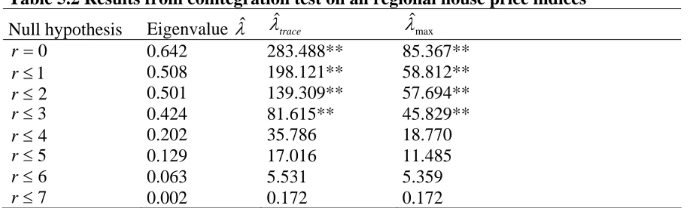
The first cointegration test looks for a common trend in the house price indices of all eight regions. The Johansen approach will in this case test for up to seven cointegrating equations and the result is presented below. Rejecting the null of up to r cointegration relationships means that there may be r+1 cointegration vectors.

Table 5.2 Results from cointegration test on all regional house price indices Null hypothesis Eigenvalue λˆ λˆtrace λˆmax

0 = r 0.642 283.488** 85.367** 1 ≤ r 0.508 198.121** 58.812** 2 ≤ r 0.501 139.309** 57.694** 3 ≤ r 0.424 81.615** 45.829** 4 ≤ r 0.202 35.786 18.770 5 ≤ r 0.129 17.016 11.485 6 ≤ r 0.063 5.531 5.359 7 ≤ r 0.002 0.172 0.172

** reject the null hypothesis at the 5 % significance level

(33)

According to the results in table 5.2, the trace test indicates four cointegrating equations as does the maximum eigenvalue statistic. It can thus be concluded that the regional house prices of Sweden are tied together by four long-run relationships, which is in line with our hypothesis stated in section 2.2. Since several of the factors affecting house prices in our model are aggregate measures, some long-run relationships between the regional house prices were expected. Some cautions in the interpretation of the results should however be considered. The Johansen test is very sensitive to the choice of lag length and which deterministic components that should be included. The economic implications and their plausibility should therefore be taken into account.19

One drawback with the Johansen approach is that we cannot tell which regions that are cointegrated. The test results in table 5.2 only tell us that four long-run relationships between some regions exist. For further investigation of which regions that are related, we have in the next section divided the regions into three groups: Northern Sweden, Middle Sweden including Stockholm and South-West of Sweden.

5.1.2.2 Cointegration between Regional House Prices: North, Middle and South

A long-run relationship is expected between the house prices in the regions which are most alike. The factor determining the resemblance tested for here and in the next section are geographical proximity and the existence of a metropolitan area in the regions. For this test, the eight regions were divided into three groups where Northern Sweden consists of RIKS6-8, Middle Sweden examines RIKS1-2 and South-Western Sweden contains the regions RIKS3-5. The results from the three Johansen tests performed are to be found in the tables below.

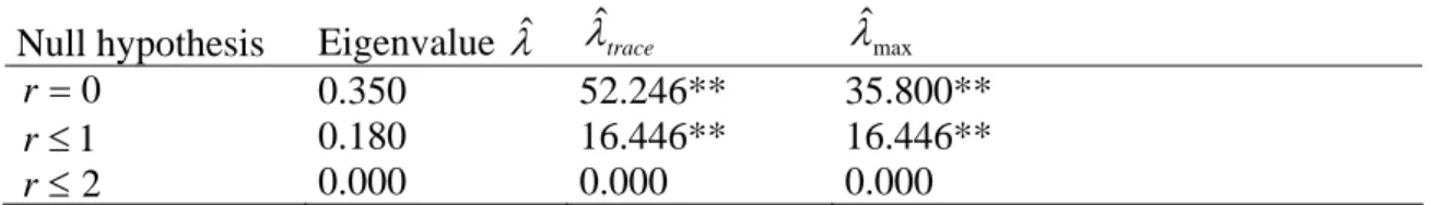
Table 5.3 Results from cointegration testing of regions in Northern Sweden

Null hypothesis Eigenvalue λˆ λˆtrace λˆmax 0 = r 0.350 52.246** 35.800** 1 ≤ r 0.180 16.446** 16.446** 2 ≤ r 0.000 0.000 0.000

The results from the regions belonging to Northern Sweden indicate that there are two cointegrating equations. This is the maximum number of cointegrating equations that three regions could experience without it being a full rank which means that the variables are

19

(34)

stationary. The presence of two long-run relationships is in line with our hypothesis and this may also be an indication that these three housing markets have many common features.

Table 5.4 Results from cointegration testing of regions in Middle Sweden

Null hypothesis Eigenvalue λˆ λˆtrace λˆmax 0 = r 0.230 22.698** 21.643** 1 ≤ r 0.013 1.055 1.055

Since Middle Sweden only consists of two regions, there can only be one cointegrating relationship and the test results confirm that the two regions share a common trend. The regions accounted for under Middle Sweden belong to the most populous areas of the country with several of the largest cities. These cities are also allocated over a geographically small area which could lead to similarities in the housing markets. The close distance allows commuting to a larger extent which could lead to the markets converging to become more like a single market.

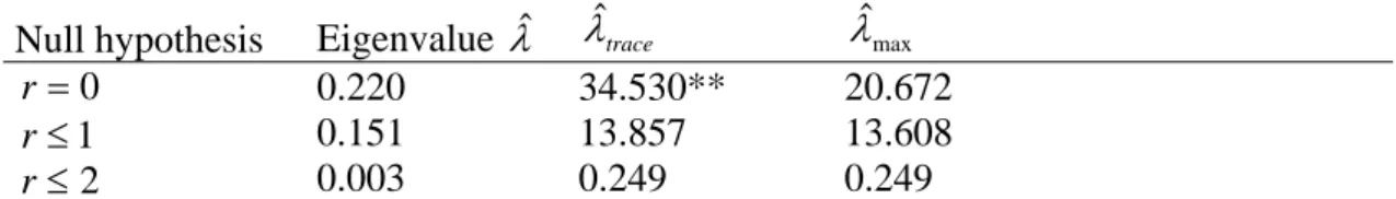
Table 5.5 Results from cointegration testing of regions in South-West of Sweden Null hypothesis Eigenvalue λˆ λˆtrace λˆmax

0 = r 0.220 34.530** 20.672 1 ≤ r 0.151 13.857 13.608 2 ≤ r 0.003 0.249 0.249

For South-West of Sweden the results are not as clear as for the two previous groups. The trace statistic indicates one cointegration equation whereas the maximum eigenvalue statistic implies that no long-run relationships exist. That the trace statistic and the maximum eigenvalue statistic leads to different conclusions regarding the number of cointegrating vectors is not uncommon and the interpretation in general of results obtained from the Johansen type cointegration tests can be difficult. One could for example use graphical examination of the cointegration relationships to help decide which statistic to adopt (Johansen and Juselius, 1992). To further refine the results for this regional grouping, cointegration tests were performed for all possible combinations of the three regions. The outcome of these tests shows that a common trend exists between RIKS3 (Småland and the Islands) and RIKS4 (Southern Sweden) which are the two most southern regions of Sweden.