Empirical Likelihood-Based NonParametric Inference for the Difference between Two Partial AUCS

(1)

Georgia State University

ScholarWorks @ Georgia State University

Mathematics Theses Department of Mathematics and Statistics

8-2-2007

Empirical Likelihood-Based NonParametric

Inference for the Difference between Two Partial

AUCS

Yan Yuan

Follow this and additional works at:https://scholarworks.gsu.edu/math_theses

Part of theMathematics Commons

This Thesis is brought to you for free and open access by the Department of Mathematics and Statistics at ScholarWorks @ Georgia State University. It has been accepted for inclusion in Mathematics Theses by an authorized administrator of ScholarWorks @ Georgia State University. For more information, please [email protected].

Recommended Citation

Yuan, Yan, "Empirical Likelihood-Based NonParametric Inference for the Difference between Two Partial AUCS." Thesis, Georgia State University, 2007.

(2)

EMPIRICAL LIKELIHOOD-BASED NONPARAMETRIC INFERENCE FOR THE DIFFERENCE BETWEEN TWO PARTIAL AUCS

by Yan Yuan

Under the direction of Gengsheng Qin

ABSTRACT

Compare the accuracy of two continuous-scale tests is increasing important when a new test is developed. The traditional approach that compares the entire areas under two Receiver Operating Characteristic (ROC) curves is not sensitive when two ROC curves cross each other. A better approach to compare the accuracy of two diagnostic tests is to compare the areas under two ROC curves (AUCs) in the interested specificity interval. In this thesis, we have proposed bootstrap and empirical likelihood (EL) approach for inference of the difference between two partial AUCs. The empirical likelihood ratio for the difference between two partial AUCs is defined and its limiting distribution is shown to be a scaled chi-square distribution. The EL based confidence intervals for the

difference between two partial AUCs are obtained. Additionally we have conducted simulation studies to compare four proposed EL and bootstrap based intervals.

INDEX WORDS: ROC curve, AUC, PAUC, Partial AUC, Empirical Likelihood, Bootstrap, Confidence Interval.

(3)

by

Yan Yuan

A Thesis submitted in partial Fulfillment of the Requirements for the Degree of Master of Science

In the College of Arts and Science Georgia State University

(4)

Copyright by Yan Yuan

(5)

by Yan Yuan

Major Professor: Dr. Gengsheng Qin Committee: Dr. Yu-Sheng Hsu

Dr. Xu Zhang

Electronic Version Approval:

Office of Graduate Studies College of Arts and Science Georgia State University August 2007

(6)

ACKNOWLEDGEMENTS

I would like to express my gratitude to my advisor Dr.Gengsheng Qin who directed and guided me through the whole process of this thesis. This thesis cannot be finished without him.

I would also like to thank the other members of my committee, Dr. Yu-Sheng Hsu and Dr. Xu Zhang who took the time to participate as proofreaders and committee members. I thank them very much for their comments and suggestions on the improvement of my thesis.

(7)

TABLE OF CONTENTS ABSTRACT...……….……….……….. i ACKNOWLEDGMENT...……….………... iv TABLE OF CONTENTS……..………... v LIST OF ABBREVIATION……..………. vi CHAPTER I INTRODUCTION……… 1

II BOOTSTRAP CONFIDENCE INTERVAL FOR THE DIFFERENCE BETWEEN TWO PARTIAL AUCS………..…… 5

III EMPIRICAL LIKELIHOOD BASED CONFIDENCE INTERVAL FOR THE DIFFERENCE BETWEEN TWO PARTIAL AUCS………... 9

IV SIMULATION STUDIES……….. 14 V DERMATOSCOPE EXAMPLE………17 VI DISCUSSION………... 19 REFERENCES……… 20 APPENDIX A SIMULATION TABLES……….. 22

B REAL DATA ANALYSIS TABLES………. 31

C S-PLUS CODE FOR SIMULATION……….. 34

(8)

LIST OF ABBREVIATION

AUC: Area under the ROC Curve

BS: Bootstrap Method

EL: Empirical Likelihood Method

FPR: False Positive Rate

PAUC: Partial Area under the ROC Curve

ROC: Receiver Operating Characteristic

TPR: True Positive Rate

1 0p

p

Δ : The difference between two partial AUCs

1 0p

p

(9)

CHAPTER I INTRODUCTION

The accuracy of a binary diagnostic test can be measured by its specificity and sensitivity. The sensitivity or true positive rate (TPR) of the test is the proportion of diseased patients who test positive. The specificity or true negative rate (TNR) of the test is the proportion of non-diseased patients who test negative.

When the outcome of a diagnostic test is continuous, a cut-off point for the positive of disease needs to be chosen to compute specificity and sensitivity of the test.

Let Y and X be the results of a continuous-scale test for a diseased and a non-diseased

subject with cumulative distribution function G and F, respectively. For a given cut-off

point c, the sensitivity and specificity of the test are defined as

) ( 1 ) (Y c G c P Se= ≥ = − ; Sp=P(X ≤c)=F(c)

respectively. When specificity is 1-p, the corresponding sensitivity of the test is

)) 1 ( ( 1 ) (p G F 1 p

R = − − − , where F−1 is the inverse function ofF.

The receiver operating characteristic (ROC) curve, denoted by R (p), is the plot

of sensitivity against the false positive rate (FPR or 1- specificity ) as the cut-off point runs through the whole range of possible test values. In fact, the non-diseased population is unknown, and the optimal cut-off point is unknown too. For a continuous-scale

diagnostic test, the area under the ROC curve (AUC), defined as 1

0R p dp( )

δ =

_∫

, is

(10)

cut-off points. The larger is the AUC, the better the diagnostic test will be. Now, the AUC is a very popular tool in diagnostic medicine.

However, the AUC has several limitations that may make it less useful for continuous diagnostic tests (Hilden, 1991). When two ROC curves cross, the two diagnostic tests can have similar AUC even though one test has higher sensitivity for certain specificities while the other test has better sensitivity for other specificities. On the other hand, in diagnostic testing, it is critical to maintain a high sensitivity in order not to miss detecting subjects with “disease” and the interest would be in the region of ROC curve corresponding only to acceptable high sensitivities. For cancer screening, only the lower tail of the ROC curve is of interest because the FPR must be very small to be acceptable (Lilienfeld, 1974). For these reasons, the partial AUC (pAUC) has been proposed as an alternative measure to the full AUC. When using the pAUC, one considers only those regions of the ROC space where data have been observed, or which correspond to clinical relevant values of sensitivity or specificity. The pAUC over the interval )(p₀,p₁ of false positive rates, denoted by

1 0p p δ , is

∫

= 1 0 1 0 ) ( p p p p R p dp δ for 0≤ p₀ < p₁ ≤1.

It can be described as the cumulative value of sensitivity for all possible values of the false positive rates in the interval(p₀,p₁) .

Let X₁,X₂, …,X_m be the test results from a random sample of non-diseased

population with distribution function F; let Y1, Y2,…,Yn be the test results from a

(11)

(2003) proposed the following nonparametric estimator for the pAUC. When the quantiles qi = F 1(1− pi)

−

(i=0, 1) are known, the pAUC can be estimated by

(

( , )

)

) ( 1 ~ 0 1 1 1 1 0 q q X I X Y I mn i i n j j m i p p =

∑

≥ ∈ = = δ .

When the quantile q_i’s are unknown, the pAUC can be estimated by

(

(ˆ ,ˆ )

)

) ( 1 ˆ 0 1 1 1 1 0 q q X I X Y I mn i i n j j m i p p =

∑

≥ ∈ = = δ

where qˆ_i =Fˆ−1(1− p_i) (i=0,1) and Fˆ is the empirical distribution of F .

Many approaches have been proposed for constructing a confidence interval for the full or partial AUC. McClish (1989), Thompson and Zucchini (1989), and Jiang, Metz, and Nishikawa (1996) proposed parametric methods for the interval estimation of the pAUC using the bi-normal model. But Walsh (1997) found that the inferences for the pAUC are sensitive to the parametric model assumption. Wieand et al (1989) proposed a generalized nonparametric method for the inference of both the full and the partial AUC. However, their method is involved in density and distribution function estimations and mathematically too complicated to be well applied in practice. Qin and Zhou (2006) proposed an Empirical Likelihood (EL) based approach for the inference on the full AUC and recommended the use of an EL-based approach when the underlying distributions for diseased and non-diseased populations are unknown. Qin, Jin and Zhou (2006) developed bootstrap and EL-based inference for pAUC and did extensive simulation studies to compare three nonparametric confidence intervals (Normal Approximation, Bootstrap, and Empirical Likelihood) for the pAUC. They also recommended the use of EL-based

(12)

approach for pAUC when the underlying distributions for diseased and non-diseased populations are unknown.

Comparing two continuous-scale diagnostic tests is increasingly important when a new test is developed and marketed (Delong 1988). How can we know which diagnostic test is better? Investigators often compare the validity of two tests based on the estimated areas under the respective ROC curves. However, the traditional way of comparing entire areas under two ROC curves is not sensitive when two ROC curves cross each other (Zhang et al., 2002). In this thesis, we propose methods to compare the partial area under the curve within a specific range of specificity for two ROC curves, non-parametric methods based on EL and bootstrap have been developed.

This thesis is organized as follows: In Chapter II, we propose two bootstrap confidence intervals for the difference between two partial AUCs. In Chapter III, we propose the EL-based intervals for the difference between two partial AUCs. In Chapter IV, we conduct simulation study to evaluate the performances of these intervals. In Chapter V, we analyze Dermatoscope Example to illustrate the proposed intervals. Finally, the conclusions are discussed in Chapter VI.

(13)

CHAPTER II

Bootstrap Confidence Interval for the Difference between Two partial AUCS

Consider two diagnostic tests Tk (k=1, 2). Both tests yield continuous

measurements and are performed on the same m non-diseased and n diseased cases. Let

1

k

X ,Xk2…Xkm be i.i.d bivariate test results from a non-diseased population with joint

distribution functionF(x₁,x₂), and let Y_k₁, Y_k₂….., Y_kn i.i.d bivariate test results from a

diseased population with joint distribution function G(y₁,y₂). Denote the marginal

distribution functions of X_ki and Y_kj by F_k and G_k, respectively. The pAUC of test

k

T (k=1, 2) over the interval (p₀,p₁) of false positive rates, denoted by

0 1 ( )k p p δ , is 1 0 1 0 ( ) ( ) p k k p p _p R p dp δ =

_∫

for 0≤ p₀ < p₁ ≤1,

where R p_k( ) 1= −G F_k( _k−1(1−p)) is the ROC curve of test T_k (k=1, 2) . The difference between two pAUCS is

1 0p p Δ = 0 1 0 1 (2) (1) p p p p

δ −δ . Our goal is to construct confidence interval

for

1 0p

p

Δ based on test results X_ki’s and Y_kj’s.

2.1 Normal Approximation Method

For one diagnostic test, Let {Y₁,Y₂, …,Y_n} and {X₁ ,X₂,…,X_m} be the results of a continuous-scale test for a diseased and a non-diseased subject with cumulative

distribution function F and G. Dodd and Pepe (2003) defined the restricted placement

value of X as ))V(X)=(1−G(x))I(X ∈(q1,q0 when assume the quantiles q1and q0 are

known. Let ˆ( ) 1 ( ) 1 y Y I n y G n j j ≤ =

∑

=

(14)

)) , ( ( )) ( ˆ 1 ( ~ 0 1 q q X I X G Vi = − i i∈ , i=1, 2, …, m. Then, ₀ ₁ ~ p p δ =

∑

= m i i V m 1 ~ 1 is the mean of m

‘sample’ restricted placement valueV~_i's. Noticing that

1 0 ~ p p δ is a two-sample U-statistic,

it follows from the asymptotic normality for U-statistic (Lehmann, 1998) that

−

∑

= m i i mn V m 1 ~ ( 1 σ δp0p1) ⎯⎯→ L N (0, 1), Where 2 2 2 1 0 1 1 mn m n

σ = σ + σ , σ₁2=Var[V(X)], σ₀2=Var [F (min(Y,q ))].₀

Since bothq1, q0are unknown, Vi

~

is still unknown. The above normal approximation cannot be directly used to produce a confidence interval for the pAUC. Therefore Qin, Jin and Zhou (2007) introduced a bootstrap method to produce a confidence interval for pAUC.

For two diagnostic tests Tk (k=1, 2), we can use Δˆp p_{0 1} =

0 1 0 1 (2) (1) ˆ ˆ p p p p δ −δ to estimate 1 0p p Δ , where ˆ 1 ( )

(

(ˆ ₁, ˆ ₀)

)

1 1 ) ( 1 0 ki ki k k n j kj m i k p p I Y X I X q q mn ≥ ∈ =

∑

= = δ , qˆ_kl =Fˆ_k−1(1−p_l)

(l = 0, 1) , and Fˆk is the empirical distribution of Fk. It can be proved that

(

0 1 0 1

)

ˆ p p p p m+n Δ − Δ ⎯⎯→L N (0, 0 1 2 p p σ ), where 0 1 2 p p

σ is the asymptotic variance of

0 1 ˆ p p Δ . Since 0 1 2 p p σ is an unknown function of k F , Gk, 1 k F− and Gk1 − , the estimation of 0 1 2 p p

σ involves in complex density and quantile

estimation. This normal approximation cannot be directly used to produce a confidence interval for the

1 0p

p

(15)

Zhou (2006) to construct confidence intervals for the difference between two partial AUCS.

2.2 Bootstrap Method

Bootstrap method is a popular non-parametric method for constructing confidence intervals of unknown parameter; it can be applied to very complex problems. In this chapter we will propose use bootstrap method to construct confidence interval for the difference between two partial AUCS.

We draw a bootstrap resample {X_k*₁, X_k*₂,…,X_km* } of size m with replacement

from{X_k₁ ,X_k₂, …,X_km} and a separate bootstrap resample { Y_k*₁, Y_k*₂, …, Y_kn*} of size

n with replacement from {Yk1, Yk2, …, Ykn}. The partial AUC can be estimated by

(

(ˆ , ˆ )

)

) ( 1 ˆ * 0 * 1 * * 1 * 1 )* ( 1 0 ki ki k k n j kj m i k p p I Y X I X q q mn ≥ ∈ =

∑

= = δ , k=1, 2, where ˆ* ˆ 1*(1 ) l k kl F p

q = − − (l = 0, 1) is the (1−p_l)-th sample quantile based on bootstrap

resample {X_k*₁, X_k*₂,…,X_km* }. Then the bootstrap estimate for the difference of two

partial AUCs can be calculated as

= Δ* 1 0 ˆ p p )* 1 ( )* 2 ( 1 0 1 0 ˆ ˆ p p p p δ δ − .

After B repetitions of above process, B bootstrap copies of *

1 0 ˆ p p Δ are obtained { * ₍ ₎ 1 0 ˆ b p p Δ : b=1, 2, …, B}.

The bootstrap estimator for the variance of

0 1 ˆ p p Δ is given by 2 * 1 * ) ( * ) ˆ ( 1 1 1 0 1 0 p p B b b p p B V Δ −Δ − =

∑

= ,

(16)

where

∑

= Δ = Δ B b b p p p p B 1 * ) ( * 1 0 1 0 ˆ 1 .

Two bootstrap (1-α )100% confidence intervals for

1 0p

p

Δ can be proposed based

on the bootstrap variance estimator V*.

First one, called BS interval is defined as follows:

( * ₁ _/₂ * 1 0p z V p − −α Δ , * ₁ _/₂ * 1 0p z V p + −α Δ ).

Second one, called BT interval is given by (Δˆ p₀p₁ −z1−α/2 V* , * 2 / 1 1 0 ˆ _z _V p p + −α Δ ).

(17)

CHAPTER III

Empirical Likelihood Based Confidence Interval for The difference between two partial AUCs

In this chapter, we will use empirical likelihood method to construct the confidence interval for the difference between two partial AUCs.

Empirical likelihood (EL) (Owen, 1990, 2001) also is a popular non-parametric method traditionally used for providing confidence intervals. The EL method has many advantages over other non-parametric methods. For example, it has better small sample performance than approaches based on normal approximation, it studentizes internally, thereby eliminating the need for a pivot. But the applications of EL method to the ROC study are relatively few. The main challenge of developing the EL-based theory for the difference between two partial AUCs is the standard EL method can’t be applied directly when the underlying distributions are unknown (Qin and Zhou 2006) and the empirical log-likelihood ratio for the partial AUC is a sum of non-independent random variables (Qin, Jin and Zhou 2006). Hence, the standard EL theory cannot be directly applied in the partial AUC setting.

For test value Xk from a “non-diseased” subject, Dodd and Pepe (2003) defined

the restricted placement value of X_k as

)) , ( ( )) ( 1 ( ) ( k k k k k1 k2 k X G X I X q q V = − ∈ , k=1, 2, where q_kl =F_k−1(1− p_l), l = 1, 2.

When the quantiles are unknown, we can use

)) ˆ , ˆ ( ( )) ( ˆ 1 ( ) ( ˆ 2 1 k k k k k k k X G X I X q q V = − ∈ , k=1, 2,

(18)

whereqˆkl Fˆk1(1 pl)

−

= − , l = 1, 2.

k

V can be interpreted as the restricted placement value of a given “non-diseased”

test value X_k, in the survival function of the results of “diseased”. It is evident that

)} , ( , { )) ( (V_k X_k p Y_k X_k X_k q_k₁ q_k₂ E = > ∈ =pAUC_k(p₀_,p₁)= ( ) 1 0 k p p δ Therefore, = Δ 1 0p p ) 1 ( ) 2 ( 1 0 1 0p p p p δ δ − =E(V₂(X₂)−V₁(X₁)).

Based on this relationship between the difference between two partial AUCs and the restricted placement valuesV X₁( ₁) and V X₂( ₂), the profile empirical likelihood for

1 0p p Δ can be defined as , 1 : sup{ ) ( 1 1 2 , 1 1 0 = = Δ

∏

∑

= = = n j ki m i kj k p p p p L

∑

− = ki m i ki V p (ˆ 1 ) ) ( 1 0 k p p δ ,

∑

− = i m i iV p ₂ 1 2 ˆ i m i iV p ₁ 1 1 ˆ

∑

= = } 1 0p p Δ , where Vˆ_ki=Vˆ_k(X_ki), i=1, 2, …, m, k=1, 2.

Then the corresponding empirical log-likelihood ratio (ELR) for

1 0p p Δ is [ 2 ) ( 1 0 = Δp p l

∑

− − = i m i V1 1 ˆ ( 2 1 log( λ (1) )) 1 0p p δ +

∑

+ − = i m i V2 1 ˆ ( 2 1 log( λ (2) ))] 1 0p p δ , where λ and ( ) 1 0 k p p

δ (k=1, 2) are the solutions of the following equations:

0 ) ˆ ( 2 1 ˆ 1 1 ₁ (1) ) 1 ( 1 1 0 1 0 = − − −

∑

= m i _i _p _p p p i V V m λ δ δ (1) 0 ) ˆ ( 2 1 ˆ 1 1 ₂ (2) ) 2 ( 2 1 0 1 0 = − + −

∑

= m i _i _p _p p p i V V m λ δ δ (2) − − +

∑

= m i _i _p _p i V V m 1 ) 2 ( 2 2 ) ˆ ( 2 1 ˆ 1 1 0 δ λ 0 1 1 0 1 ) 1 ( 1 1 ) ˆ ( 2 1 ˆ 1 p p m i _i _p _p i V V m

∑

= − λ −δ =Δ (3)

(19)

Theorem 3.1: If

1 0p

p

Δ is the true value of the difference between two partial AUCs, and

,

lim_{m n} m

n ρ

→∞ = is a constant, then the limiting distribution of l(Δp0p1) is a scaled

chi-square distribution with one degree of freedom.

) ( 1 0p p C Δ ( ) 1 0p p l Δ ⎯⎯→χ12 L , where ( ) 1 0p p C Δ = 0 1 0 1 0 1 (1) 2 (2) 2 2 ( ) / /( ) p p p p p p m m n σ σ σ + + , 0 1 ( ) 2 [ ( )] k p p Var V Xk k σ = , k = 1, 2.

Using Theorem 3.1, two empirical and bootstrap based intervals for the difference between two partial AUCs can be constructed as follows:

The first hybrid empirical and bootstrap interval (EL) is defined as

0 1 0 1 ( _{p p} ) { _{p p} : R_α Δ = Δ ˆ( ) 1 0p p C Δ ( ) 1 0p p l Δ ≤χ₁2(1−α)},

where )χ12(1−α is the (1-α )-th quantile of the chi-square distribution

2 1 χ , ˆ( ) 1 0p p C Δ is an estimate for ( ) 1 0p p C Δ : ) ( ˆ 1 0p p C Δ = _* 2 ) 2 ( 2 ) 1 ( / ) ˆ ˆ ( 1 0 1 0 V m p p p p σ σ + , 2 1 1 2 ) ( ) ˆ 1 ˆ ( 1 1 ˆ 1 0

∑

= = − − = m i ki m i ki k p p V m V m σ , k=1, 2,

and V* is the bootstrap variance estimate defined in chapter II.

0 1

( _{p p} )

R_α Δ is an approximate confidence intervals for the difference between two

partial AUCs with asymptotically correct coverage probability 1-α, i.e.,

∈ Δ 1 0 ( _p _p P 0 1 ( _{p p}) R_α Δ ) = 1-α+ο(1).

(20)

We can solve the following equations to get the lower and upper bounds of the confidence interval for the difference between the two partial AUCs:

0 ) ˆ ( 2 1 ˆ 1 1 ) 1 ( 1 ) 1 ( 1 1 0 1 0 = − − −

∑

= m i _i _p _p p p i V V m λ δ δ (2) − − +

∑

= m i _i _p _p i V V m 1 ₂ (2) 2 ) ˆ ( 2 1 ˆ 1 1 0 δ λ 0 1 1 0 1 ₁ (1) 1 ) ˆ ( 2 1 ˆ 1 p p m i _i _p _p i V V m

∑

= − λ −δ =Δ (3) ˆ( ) 1 0p p C Δ ( ) 1 0p p l Δ =χ12(1−α) (4)

In these four equations, λ and ( )

1 0 k p p δ (k=1, 2) and 1 0p p

Δ are unknown and can be solved.

The

1 0p

p

Δ will have two solutions. The smaller one is the lower bound of the EL interval

and larger one is the upper bound of the EL interval.

The second hybrid empirical and bootstrap interval (HBEL) is given by

0 1 0 1 * ( _{p p}) { _{p p} : R_α Δ = Δ ˆ ( ) 1 0 * p p C Δ ( ) 1 0p p l Δ ≤χ₁2(1−α)}, where )ˆ ( 1 0 * p p C Δ = 0 1 0 1 *(1) 2 *(2) 2 * ˆ ˆ ( _{p p} _{p p} ) /m V σ +σ , 0 1 *( ) 2 ˆ_{p p}k

σ is the mean of B bootstrap copies of

0 1 ( ) 2

ˆ k p p

σ ( k=1,2), and V* is the bootstrap variance estimate defined in chapter II.

Similarly,

0 1 *

( _{p p} )

R_α Δ is an approximate confidence intervals for the difference

between two partial AUCs with asymptotically correct coverage probability 1-α, i.e.,

∈ Δ 1 0 ( _p _p P 0 1 * ( _{p p} ) R_α Δ ) = 1-α+ο(1).

(21)

The lower and upper bound of HBEL interval can be obtained by solving the following

equations: 0 ) ˆ ( 2 1 ˆ 1 1 ) 1 ( 1 ) 1 ( 1 1 0 1 0 = − − −

∑

= m i _i _p _p p p i V V m λ δ δ (6) − − +

∑

= m i _i _p _p i V V m 1 ₂ (2) 2 ) ˆ ( 2 1 ˆ 1 1 0 δ λ 0 1 1 0 1 ₁ (1) 1 ) ˆ ( 2 1 ˆ 1 p p m i _i _p _p i V V m

∑

= − λ −δ =Δ (7) ) ( ˆ 1 0 * p p C Δ ( ) 1 0p p l Δ 2(1 ) 1 α χ − = (8)

(22)

CHAPTER IV Simulation Study

In this chapter, we conduct a simulation study to evaluate coverage accuracy and interval length of the newly proposed four intervals for the difference

1 0p

p

Δ of two

pAUCs. In the study, the difference

1 0p

p

Δ between two pAUCs is taken to be 0 and 0.2.

We generate 1000 random samples of size n from G(y₁,y₂) for test responses of

diseased patients, and another set of independent random samples of size m from

) , (x₁ x₂

F for test responses of non-diseased patients.

The distributionF(x₁,x₂) is chosen to be a bivariate normal distribution having

meansE(X₁)=0, E(X₂)=0 with a common standard deviation 1 and correlationρ.

The distribution G(y1,y2) is chosen to be a bivariate normal distribution having

meansE(Y1)=μ1, E(Y2)=μ2 with a common standard deviation 2 and correlationρ. μ1

and μ2 are calculated by solving the following equations

1 0 1 0 ( ) ( ) p k k p p _p R p dp δ =

∫

with R pk( ) 1 G Fk( k1(1 p)) − = − − , k = 1, 2. When 1 0p p

Δ = 0, we choose three groups of

0 1 0 1 (1) (2)

ˆ ˆ

(δ_{p p} ,δ_{p p} ) to calculate three groups of

(μ₁, μ₂) and generate random samples from the G(y₁,y₂): (i) δ_(0,0.4)(2) =δ_(0,0.4)(1) =0.2 with (p₀,p₁) = (0, 0.4), (ii) δ_(0,0.7)(2) =δ_(0,0.7)(1) =0.45 with (p0,p1) = (0, 0.7),

(iii) (2) (1)

(0.05,0.50) (0.05,0.50) 0.26

(23)

When

1 0p

p

Δ = 0.2, we also choose three groups of

0 1 0 1 (1) (2)

ˆ ˆ

(δ_{p p} ,δ_{p p} ) to calculate three groups

of (μ₁, μ₂) and generate random samples from the G(y₁,y₂): (i) δ_(0,0.4)(2) =0.37,δ_(0,0.4)(1) =0.17 with (p₀,p₁) = (0, 0.4), (ii) δ_(0,0.7)(2) =0.61,δ_(0,0.7)(1) =0.41 with (p0,p1) = (0, 0.7),

(iii) (2) (1)

(0.05,0.50) 0.39, (0.05,0.50) 0.19

δ = δ = with (p₀,p₁) = (0.05, 0.50).

In the bootstrap step, we draw B = 150 bootstrap re-samples from the original samples. We construct both 90% and 95% confidence intervals for

1 0p

p

Δ . The results of the

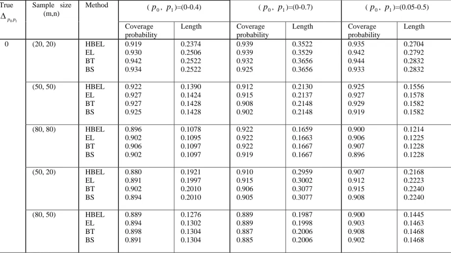
simulation study are shown in Table I to Table VIII. From these tables, the following observations were made.

(1) When the correlation ρ= 0 and

1 0p

p

Δ = 0, the four proposed intervals have

similar coverage probabilities but the hybrid empirical likelihood and bootstrap intervals (EL and HBEL) have slightly shorter interval length.

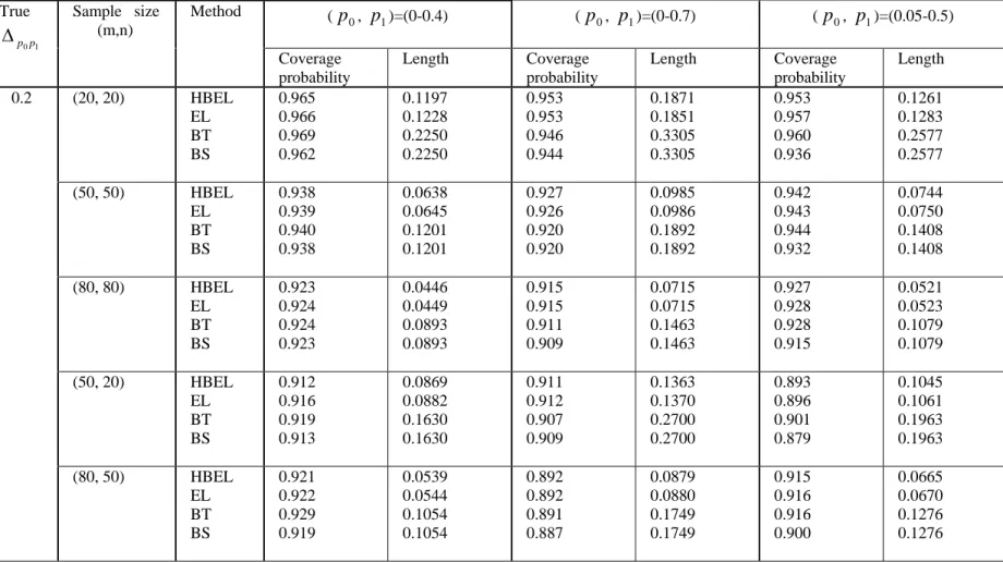
(2) When

1 0p

p

Δ > 0, all the intervals over-cover the true difference between two

pAUCs when sample sizes are small. As the sample sizes increase, the coverage probabilities of all the intervals approach to the nominal level. Although in most time all the interval have similar coverage probabilities, the EL and HBEL intervals have much shorter interval length than bootstrap (BS and BT) intervals.

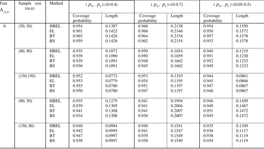
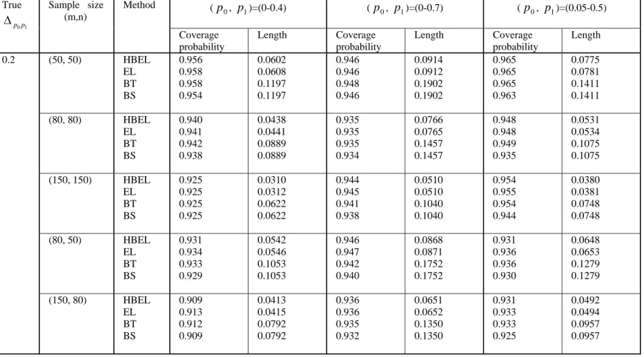
(3) When the correlation is positive (ρ = 0.3), bigger sample sizes (m, n ≥ 150)

are needed to get better coverage accuracy for all the intervals.

In summary, the simulation study indicates that the hybrid empirical likelihood and bootstrap based intervals perform better than the bootstrap intervals when two partial AUCs are different. When there is no difference between two partial AUCs, the four

(24)

proposed intervals have similar performance. Therefore, we recommend the use of hybrid empirical likelihood and bootstrap method for construction of confidence interval of difference between two pAUCs when the underlying distributions for diseased and non-diseased populations are unknown.

(25)

CHAPTER V Dermatoscope Example

Malignant melanoma (MM) is one of the most deadly kinds of skin disease. Melanomas of less than 1mm are not likely to have spread to the lymph nodes or to other parts of the body, called early stage; they have a very good chance of cure. The thinner the melanoma, the better chance of a complete cure. Early diagnosis of malignant melanoma is essential for cure.

Dermatoscopy is a hand- held instrument for skin surface microscopy at 10 times magnification and is a noninvasive diagnostic technique for the early diagnosis of melanoma and the evaluation of other pigmented and non-pigmented lesions on the skin that are not as well seen with the unaided eye [www.medterms.com]. Stolz et al (1994) studied the accuracy of clinical evaluations with or without the aid of Dermatoscopy in detecting MM by using the ABCD rule (Asymmetry, irregular border, different colors, and Diameter larger than 6mm). In this study, two tests were applied for detecting MM; the first test is the clinical assessment without the aid of dermatoscopy, and the second test is the clinical assessment with the aid of dermatoscopy. The data set we used here includes 21 patients with MM and 51 patients with benign melanocytic lesions; all patients have both tests results. The objective of this study is to find out whether the aid of dermatoscopy can improve for detecting MM. We estimate the difference of two pAUCs of the two tests and construct confidence intervals for the difference by using the proposed methods. The 90% and 95% confidence intervals for the difference between two pAUCs over three intervals of FPR are shown in Table IX and Table X.

(26)

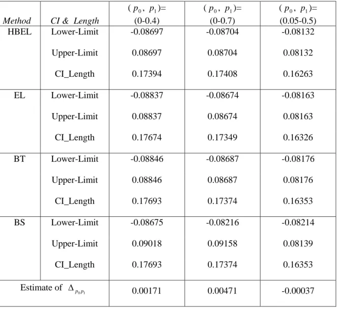
The estimates of the differences between two pAUCs over the three intervals (0, 0.4), (0, 0.7) and (0.05, 0.50) of FPR for the two tests are all close to 0. Also, all the confidence intervals for the differences contain zero. Therefore, we conclude that there is no significant advantage in adopting the clinical assessment with the aid of dermatoscopy in detecting MM. The same conclusion has been obtained in Qin, Hsu and Zhou (2006) where they compared those two tests by using the sensitivities at a fixed level of specificity.

(27)

CHAPTER VI Discussion and Conclusion

Comparing the accuracy of two continuous-scale tests is increasingly important when a new test is developed and marketed. There are many ways to do such a comparison. For example, we can compare the sensitivities at a fixed common specificity or we can compare the areas under the ROC curves. But traditional ways of comparing entire areas under two ROC curves are not sensitive when two ROC curves cross each other. Comparing the areas under two ROC curves on the interested FPR interval is a more appropriate way to compare the accuracy of two diagnostic tests. In this thesis, we have proposed two bootstrap based confidence intervals (BS and BT) and two hybrid empirical likelihood and bootstrap confidence intervals (EL and HBEL). The simulation study indicates that two hybrid empirical likelihood and bootstrap intervals performed better than the bootstrap intervals in most cases, especially when there is a difference between two pAUCs. The proposed hybrid empirical likelihood and bootstrap based method combines the power of both bootstrap and empirical likelihood methods. The unknown scale constant in the empirical likelihood theorem can be conveniently and accurately estimated by using bootstrap method. The confidence intervals can be constructed by using the empirical likelihood theorem. Based on this study, we recommend the use of the proposed hybrid empirical likelihood and bootstrap confidence intervals for the difference between two partial AUCs when the underlying distributions for diseased and non-diseased populations are unknown.

(28)

REFERENCES

Bamber DC (1975). The area above the ordinal dominance graph and the area below the

receiver operating characteristic curve graph. Journal of Mathematical Psychology,

12:387-415.

Cai T and Dodd L (2006). Regression analysis for the partial area under the ROC curve. Harvard University Biostatistics Working Paper Series.

DeLong ER, DeLong DM, Clarke-Pearson DL (1988). Comparing the areas under two or more correlated receiver operating characteristic curves: a nonparametric approach.

Biometrics. 44:837-45.

Dodd L and Pepe MS (2003). Partial AUC Estimation and Regression. Biometrics. 59:

614-623.

Hanley JA, McNeil BJ (1983). A method of comparing the areas under receiver

operating characteristic curves derived from the same cases. Radiology.148:839-43.

Hilden J (1991). The area under the ROC curve and its competitors. Medical Decision

making 11:95-101.

Jiang Y, Metz CE and Nishikawa RM (1996). A receiver operating characteristic partial

area index for highly sensitive diagnostic tests. Radiology 143:29-36.

Lilienfeld AM (1974). Some limitations and problems of screening for cancer. Cancer

36:1720-1724

McClish DK (1989). Analyzing a portion of the ROC curve. Medical Decision Making9:

190–195.

Molodianovitch K, Faraggi D, Reiser B (2006). Comparing the areas under two

correlated ROC curves: parametric and non-parametric approaches. Biom J.48:745-57

Owen A. (2001). Empirical likelihood. Chapman & Hall/CRC, New York.

Pepe MS and Cai T (2002). The analysis of placement values for evaluating

discriminatory measures. Biometrics60:528-535.

Pepe MS (2003). The statistical evaluation of medical tests for classification and biomarkers. Oxford University Press, Cary, NC.

Pepe MS (2003). The statistical evaluation of diagnostic tests and prediction. Oxford University Press, Cary, NC.

(29)

Qin, GS and Zhou XH (2006). Empirical Likelihood Inference for the Area Under the

ROC Curve. Biometrics 62: 613-622.

Qin, GS, Hsu, YS, and Zhou, XH (2006). New confidence intervals for the difference

between two sensitivities at a fixed level of specificity. Statistics in Medicine 25:

3487-3502.

Qin, GS, Jin, XP and Zhou, XH (2006). Bootstrap and Empirical Likelihood-based

inference for the Partial Area Under the ROC Curve. Manuscript.

Shapiro DE (1999). The Interpretation of Diagnostic Tests. Statistical Methods in

Medical Research,8:113-134

Thompson ML, and Zucchini W (1989). On the statistical analysis of ROC curvers.

Statistics in Medicine. 8:1277-1290.

Wieand S (1989). A Family of Non-Parametric Statistic for Comparing Diagnostic

Markers with Paired or Unpaired Data. Biometrika, 76:585-592

Walsh SJ(1997). Limitations to the robustness of binormal ROC curves: effects of model misspecification and location of the decision thresholds on bias, precision, size and

power. Statistics in Medicine. 16: 669-679

Zhang DD, Zhou XH, Freeman DH and Freeman JL(2002). A non-parametric method for the comparison of partial areas under ROC curves and its application to large health care data sets. Statistics in Medicine. 21:701-15

(30)

APPENDIX

(31)

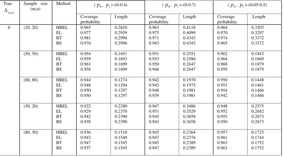
Table I: Level of 95 per cent confidence interval for

1 0p p

Δ . Bivariate normal distribution with ρ =0.

(p₀, p₁)=(0-0.4) (p₀, p₁)=(0-0.7) (p₀, p₁)=(0.05-0.5) True 1 0p p Δ Sample size (m,n) Method Coverage probability Length Coverage probability Length Coverage probability Length (20, 20) HBEL EL BT BS 0.965 0.977 0.981 0.976 0.2810 0.2959 0.2996 0.2996 0.963 0.975 0.971 0.963 0.4118 0.4099 0.4343 0.4343 0.964 0.970 0.974 0.965 0.3203 0.3297 0.3372 0.3372 (50, 50) HBEL EL BT BS 0.954 0.959 0.963 0.958 0.1651 0.1693 0.1699 0.1699 0.951 0.953 0.950 0.946 0.2551 0.2586 0.2647 0.2647 0.962 0.964 0.968 0.959 0.1843 0.1869 0.1879 0.1879 (80, 80) HBEL EL BT BS 0.944 0.948 0.950 0.950 0.1274 0.1294 0.1297 0.1297 0.942 0.943 0.940 0.939 0.1970 0.1975 0.1981 0.1981 0.950 0.951 0.954 0.942 0.1448 0.1461 0.1466 0.1466 (50, 20) HBEL EL BT BS 0.922 0.929 0.942 0.938 0.2280 0.2370 0.2390 0.2390 0.947 0.951 0.945 0.943 0.3486 0.3529 0.3658 0.3658 0.948 0.952 0.955 0.950 0.2575 0.2642 0.2673 0.2673 0 (80, 50) HBEL EL BT BS 0.936 0.943 0.947 0.937 0.1510 0.1540 0.1545 0.1545 0.945 0.947 0.945 0.947 0.2364 0.2376 0.2389 0.2389 0.957 0.961 0.963 0.963 0.1725 0.1744 0.1752 0.1752

(32)

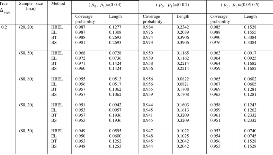
Table II: Level of 95 per cent confidence interval for

1 0p p

(p₀, p₁)=(0-0.4) (p₀, p₁)=(0-0.7) (p₀, p₁)=(0.05-0.5) True 1 0p p Δ Sample size (m,n) Method Coverage probability Length Coverage probability Length Coverage probability Length (20, 20) HBEL EL BT BS 0.987 0.987 0.988 0.981 0.1277 0.1308 0.2693 0.2693 0.984 0.976 0.974 0.973 0.2342 0.2089 0.3906 0.3906 0.985 0.988 0.990 0.976 0.1528 0.1555 0.3084 0.3084 (50, 50) HBEL EL BT BS 0.968 0.972 0.971 0.960 0.0728 0.0736 0.1424 0.1424 0.959 0.959 0.958 0.956 0.1165 0.1162 0.2214 0.2214 0.963 0.964 0.964 0.959 0.0917 0.0925 0.1682 0.1682 (80, 80) HBEL EL BT BS 0.955 0.956 0.957 0.957 0.0513 0.0517 0.1062 0.1062 0.956 0.956 0.955 0.959 0.0822 0.0821 0.1708 0.1708 0.965 0.967 0.969 0.963 0.0602 0.0605 0.1281 0.1281 (50, 20) HBEL EL BT BS 0.951 0.953 0.957 0.953 0.0942 0.0957 0.1936 0.1936 0.944 0.945 0.941 0.945 0.1603 0.1613 0.3209 0.3209 0.958 0.959 0.961 0.951 0.1243 0.1262 0.2332 0.2332 0.2 (80, 50) HBEL EL BT BS 0.949 0.950 0.953 0.948 0.0595 0.0600 0.1252 0.1253 0.947 0.948 0.945 0.944 0.1022 0.1025 0.2042 0.2042 0.953 0.954 0.956 0.953 0.0740 0.0745 0.1528 0.1528

(33)

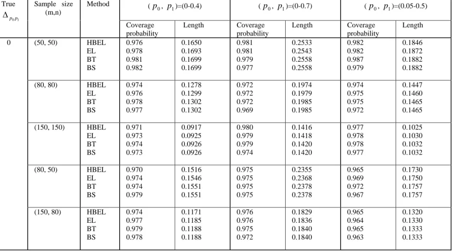
Table III: Level of 95 per cent confidence interval for

1 0p p

Δ . Bivariate normal distribution with ρ =0.3.

(34)

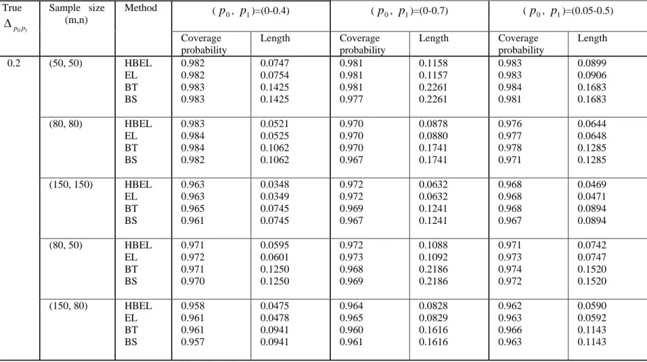
Table IV: Level of 95 per cent confidence interval for

1 0p p

(p0, p1)=(0-0.4) (p0, p1)=(0-0.7) (p0, p1)=(0.05-0.5) True 1 0p p Δ Sample size (m,n) Method Coverage probability Length Coverage probability Length Coverage probability Length (50, 50) HBEL EL BT BS 0.982 0.982 0.983 0.983 0.0747 0.0754 0.1425 0.1425 0.981 0.981 0.981 0.977 0.1158 0.1157 0.2261 0.2261 0.983 0.983 0.984 0.981 0.0899 0.0906 0.1683 0.1683 (80, 80) HBEL EL BT BS 0.983 0.984 0.984 0.982 0.0521 0.0525 0.1062 0.1062 0.970 0.970 0.970 0.967 0.0878 0.0880 0.1741 0.1741 0.976 0.977 0.978 0.971 0.0644 0.0648 0.1285 0.1285 (150, 150) HBEL EL BT BS 0.963 0.963 0.965 0.961 0.0348 0.0349 0.0745 0.0745 0.972 0.972 0.969 0.967 0.0632 0.0632 0.1241 0.1241 0.968 0.968 0.968 0.967 0.0469 0.0471 0.0894 0.0894 (80, 50) HBEL EL BT BS 0.971 0.972 0.971 0.970 0.0595 0.0601 0.1250 0.1250 0.972 0.973 0.968 0.969 0.1088 0.1092 0.2186 0.2186 0.971 0.973 0.974 0.972 0.0742 0.0747 0.1520 0.1520 0.2 (150, 80) HBEL EL BT BS 0.958 0.961 0.961 0.957 0.0475 0.0478 0.0941 0.0941 0.964 0.965 0.960 0.961 0.0828 0.0829 0.1616 0.1616 0.962 0.963 0.966 0.963 0.0590 0.0592 0.1143 0.1143

(35)

Table V: Level of 90 per cent confidence interval for

1 0p p

(36)

Table VI: Level of 90 per cent confidence interval for

1 0p p

(37)

Table VII: Level of 90 per cent confidence interval for

1 0p p

(p₀, p₁)=(0-0.4) (p₀, p₁)=(0-0.7) (p₀, p₁)=(0.05-0.5) True 1 0p p Δ Sample size (m,n) Method Coverage probability Length Coverage probability Length Coverage probability Length (50, 50) HBEL EL BT BS 0.954 0.961 0.965 0.959 0.1387 0.1422 0.1426 0.1426 0.966 0.966 0.964 0.962 0.2138 0.2146 0.2154 0.2154 0.954 0.956 0.957 0.953 0.1550 0.1572 0.1578 0.1578 (80, 80) HBEL EL BT BS 0.935 0.939 0.939 0.936 0.1072 0.1090 0.1091 0.1091 0.950 0.950 0.948 0.945 0.1654 0.1659 0.1662 0.1662 0.949 0.951 0.952 0.949 0.1219 0.1230 0.1233 0.1233 (150,150) HBEL EL BT BS 0.952 0.953 0.955 0.950 0.0772 0.0779 0.0780 0.0780 0.953 0.954 0.951 0.947 0.1193 0.1195 0.1197 0.1197 0.944 0.945 0.947 0.946 0.0861 0.0866 0.0867 0.0867 (80, 50) HBEL EL BT BS 0.935 0.939 0.941 0.934 0.1279 0.1305 0.1308 0.1308 0.941 0.941 0.941 0.936 0.1994 0.2004 0.2007 0.2007 0.946 0.949 0.951 0.945 0.1450 0.1467 0.1472 0.1472 0 (150, 80) HBEL EL BT BS 0.940 0.942 0.947 0.938 0.0984 0.0995 0.0997 0.0997 0.940 0.941 0.939 0.938 0.1541 0.1547 0.1549 0.1549 0.935 0.936 0.938 0.934 0.1109 0.1117 0.1119 0.1119

(38)

Table VIII: Level of 90 per cent confidence interval for

1 0p p

(39)

(40)

Table IX: Dermatoscope Example Level of 95 per cent confidence interval for

1 0p

p

Δ

Method CI & Length

(p0, p1)= (0-0.4) (p0, p1)= (0-0.7) (p0, p1)= (0.05-0.5) HBEL Lower-Limit -0.10722 -0.11170 -0.09468 Upper-Limit 0.10722 0.11170 0.09468 CI_Length 0.21444 0.22340 0.18936 EL Lower-Limit -0.10913 -0.11129 -0.09512 Upper-Limit 0.10913 0.11129 0.09512 CI_Length 0.21826 0.22258 0.19024 BT Lower-Limit -0.10931 -0.11155 -0.09533 Upper-Limit 0.10931 0.11155 0.09533 CI_Length 0.21862 0.22310 0.19066 BS Lower-Limit -0.10945 -0.11714 -0.10025 Upper-Limit 0.10917 0.10596 0.09041 CI_Length 0.21862 0.22310 0.19066 Estimate of 1 0p p Δ _{-0.00014 -0.00559 -0.00492}

(41)

Table X: Dermatoscope Example Level of 90 per cent confidence interval for

1 0p

p

Δ

Method CI & Length

(p₀, p₁)= (0-0.4) (p₀, p₁)= (0-0.7) (p₀, p₁)= (0.05-0.5) HBEL Lower-Limit -0.08697 -0.08704 -0.08132 Upper-Limit 0.08697 0.08704 0.08132 CI_Length 0.17394 0.17408 0.16263 EL Lower-Limit -0.08837 -0.08674 -0.08163 Upper-Limit 0.08837 0.08674 0.08163 CI_Length 0.17674 0.17349 0.16326 BT Lower-Limit -0.08846 -0.08687 -0.08176 Upper-Limit 0.08846 0.08687 0.08176 CI_Length 0.17693 0.17374 0.16353 BS Lower-Limit -0.08675 -0.08216 -0.08214 Upper-Limit 0.09018 0.09158 0.08139 CI_Length 0.17693 0.17374 0.16353 Estimate of 1 0p p Δ _{0.00171 0.00471 -0.00037}

(42)

APPENDIX C: The Splus code for simulation studies

#######################part 1: Functions#####################

## Function R(p)##

Rp<-function(p, muy, stdd) 1-pnorm(qnorm(1-p),muy, stdd)

## solveNonlinear##

##nlmin can be used to solve a system of nonlinear equations: solveNonlinear <- function(f, y0, x, ...){

# solve f(x) = y0

# x is vector of initial guesses, same length as y0 # ... are additional arguments to nlmin (not to f) g <- function(x, y0, f) sum((f(x) - y0)^2)

g$y0 <- y0 # set g's default value for y0 g$f <- f # set g's default value for f

nlmin(g, x, max.fcal = 10000, max.iter = 10000, ...) }

##calculate x[1]=y1.mean x[2]=y2.mean## mu <- function(x){

c( integrate(Rp, muy=x[1], stdd=y1.sd, lower=p0, upper = p1)$integral, integrate(Rp, muy=x[2], stdd=y2.sd, lower=p0, upper = p1)$integral ) }

##function for sigma##

my.mean <- function(vv) mean((vv-mean(vv))^2) ;

##solve x[1]: p0p1.1 x[2]: p0p1.2 x[3]: lamda

f <- function(x) c( mean((V.hat[,1]-x[1])/(1-2*x[3]*(V.hat[,1]-x[1]))), mean((V.hat[,2]-x[2])/(1+2*x[3]*(V.hat[,2]-x[2]))),

mean(V.hat[,2]/(1+2*x[3]*(V.hat[,2]-x[2])))-mean(V.hat[,1]/(1-2*x[3]*(V.hat[,1]-x[1]))))

##x[1]: p0p1.1 x[2]: p0p1.2 x[3]: lamda x[4]: delta using C.deltap0p1.hat g2 <- function(x) c( mean((V.hat[,1]-x[1])/(1-2*x[3]*(V.hat[,1]-x[1]))), mean((V.hat[,2]-x[2])/(1+2*x[3]*(V.hat[,2]-x[2]))), mean(V.hat[,2]/(1+2*x[3]*(V.hat[,2]-x[2])))-mean(V.hat[,1]/(1-2*x[3]*(V.hat[,1]-x[1])))-x[4], C.deltap0p1.hat*(2*(sum( log(abs(1-2*x[3]*(V.hat[,1]-x[1]))))+sum( log(abs(1+2*x[3]*(V.hat[,2]-x[2]))))))-CritVal)

##x[1]: p0p1.1 x[2]: p0p1.2 x[3]: lamda x[4]: delta using C.deltap0p1 g1 <- function(x) c( mean((V.hat[,1]-x[1])/(1-2*x[3]*(V.hat[,1]-x[1]))), mean((V.hat[,2]-x[2])/(1+2*x[3]*(V.hat[,2]-x[2]))), mean(V.hat[,2]/(1+2*x[3]*(V.hat[,2]-x[2])))-mean(V.hat[,1]/(1-2*x[3]*(V.hat[,1]-x[1])))-x[4], C.deltap0p1*(2*(sum( log(abs(1-2*x[3]*(V.hat[,1]-x[1]))))+sum( log(abs(1+2*x[3]*(V.hat[,2]-x[2]))))))-CritVal)

##function for deltapAUC.hat##

deltapAUC <- function(X1X2, Y1Y2, p0, p1, m){

# Caculate X Quantile of 1-pi (i=0,1) for q.hat q0.1.hat<-quantile(X1X2[,1],1-p0);

(43)

q1.1.hat<-quantile(X1X2[,1],1-p1); q1.2.hat<-quantile(X1X2[,2],1-p1);

# Caculate V(ki).hat & C(deltap0p1).hat V.hat<-matrix(, m, 2) for (i in 1 : m){ V.hat[i,1]<-(1-mean(Y1Y2[,1]<= X1X2[i,1]))*(q1.1.hat <= X1X2[i,1])*(X1X2[i,1]<=q0.1.hat) V.hat[i,2]<-(1-mean(Y1Y2[,2]<= X1X2[i,2]))*(q1.2.hat <= X1X2[i,2])*(X1X2[i,2]<=q0.2.hat) } delta.pAUC.hat<-mean(V.hat[,2])-mean(V.hat[,1]) C.deltap0p1.hat<-(my.mean(V.hat[,1])+my.mean(V.hat[,2]))/(m*Vstar)

list(delta.pAUC.hat, C.deltap0p1.hat, V.hat) }

##bootstrap function##

booth.trap <- function(B, X1X2, Y1Y2, m, n, p0, p1){ delta.pAUC<-0;

sigma <- matrix(,B, 2) for (b in 1:B) {

X1B <- sample(X1X2[,1], m, replace = T) X2B <- sample(X1X2[,2], m, replace = T) Y1B <- sample(Y1Y2[,1], n, replace = T) Y2B <- sample(Y1Y2[,2], n, replace = T)

q0B.1.hat<-quantile(X1B, c(1-p0)) # hatq0, hatq1: sample quantiles of F q0B.2.hat<-quantile(X2B, c(1-p0)) # hatq0, hatq1: sample quantiles of F q1B.1.hat<-quantile(X1B, c(1-p1)) q1B.2.hat<-quantile(X2B, c(1-p1)) VB <- matrix(,m, 2) for (i in 1:m) {

VB[i,1]<- (1-mean(Y1B <= X1B[i])) *(q1B.1.hat <= X1B[i])*(X1B[i] <= q0B.1.hat) VB[i,2]<- (1-mean(Y2B <= X2B[i])) *(q1B.2.hat <= X2B[i])*(X2B[i] <= q0B.2.hat) } sigma[b,1]<-my.mean(VB[,1]) sigma[b,2]<-my.mean(VB[,2]) delta.pAUC[b]<-mean(VB[,2])-mean(VB[,1]) } list(delta.pAUC, sigma) }

########################### End function part ####################

########################### Part2: initial value################## iter<-1000 B=150 rho=0 #rho=0.3 m<-50; n<-20; y1.sd<-2; y2.sd<-2; levelc<-0.95 #levelc<-0.90

(44)

CritVal<-qchisq(levelc,1) Z<-qnorm(1-(1-levelc)/2) y1.mean<-y2.mean<-0 p0<-0 ; p1<-0.4 pAUC1 <- 0.2 pAUC2 <- 0.2 deltapAUC.true<- pAUC2-pAUC1

S<-solveNonlinear(mu, c( pAUC1, pAUC2), c(0.1, 0.1)) y1.mean<-S$x[1] y2.mean<-S$x[2] #################### End part2 ####################### #################### Part3: Loop ################### CovCount<-c(0,0,0,0) CIL<-c(0,0,0) #LP<-c(0,0,0,0) #UP<-c(0,0,0,0)

for ( i12 in c(1:iter)){

# generate non-diseased population F(X1, X2)

# the sample from 2-dimensinal multinormal distribution with mean 0 and std=1 X1X2<-rmvnorm(m, mean=c(0,0), cov=matrix(c(1,rho,rho,1),2))

# generate diseased population G(Y1,Y2)

# the sample from 2-dimensinal multinormal distribution with mean #(y1.mean,y2.mean) and std=(y1.sd,y2.sd)

Y1Y2<-rmvnorm(n, mean=c(y1.mean,y2.mean),

cov=matrix(c(y1.sd^2,rho*y1.sd*y2.sd, rho*y1.sd*y2.sd, y2.sd^2),2))

##### 1. bootstrap ######

boot.list<- booth.trap(B, X1X2, Y1Y2, m, n, p0, p1)

delta.pAUC <- boot.list[[1]] sigma <- boot.list[[2]]

delta.pAUCbar.B<-mean(delta.pAUC); delta.pAUCbar.B # Estimate mean difference of two pAUCs by bootstrap

Vstar<-var(delta.pAUC); #Variance of delta.pAUC by bootstrap

C.deltap0p1<-(mean(sigma[,1])+mean(sigma[,2]))/(m*Vstar);

#####END OF BOOTSTRAP#######

###### 2. Caculate delta.pAUC.hat######

delta.pAUC.hat.list <- deltapAUC(X1X2, Y1Y2, p0, p1, m)

delta.pAUC.hat <- delta.pAUC.hat.list[[1]] C.deltap0p1.hat <- delta.pAUC.hat.list[[2]] V.hat <- delta.pAUC.hat.list[[3]]

(45)

###### 3. caculate L.deltap0p1###### # EL Method # #x[1]: p0p1.1 x[2]: p0p1.2 x[3]: lamda x<-solveNonlinear(f, c( 0,0, deltapAUC.true), c(0.1, 0.2, 0)) p0p1.1<-x$x[1]; p0p1.2<-x$x[2]; lamda<-x$x[3]; l.delta.p0p1<-2*(sum( log(1-2*lamda*(V.hat[,1]-p0p1.1)))+sum( log(1+2*lamda*(V.hat[,2]-p0p1.2)))) Vel<-C.deltap0p1*l.delta.p0p1; Vel.hat<-C.deltap0p1.hat*l.delta.p0p1; ####END OF 3. ######

###### 4. Caculate C.I and coverage######

## compute the HBEL interval(Vel from bootstrap)## if (Vel <= CritVal)

CovCount[1]<-CovCount[1]+1

#x[1]: p0p1.1 x[2]: p0p1.2 x[3]: lamda x[4]: delta

bd<-solveNonlinear(g1, c( 0,0,0,0), c(0.3, 0.1, 0.001, -0.9)) #low.HBEL<-bd$x[4] # lower limit of the CI

b<-solveNonlinear(g1, c( 0,0,0,0), c(0.1, 0.3, 0.001, 0.999)) #up.HBEL<-b$x[4] # upper limit of the CI

#low and up band HBEL #LP[1]<- LP[1]+bd$x[4] #UP[1]<- UP[1]+ b$x[4]

# The length of HBEL CI

CIL[1]<- CIL[1]+(b$x[4]- bd$x[4])

## compute the EL interval(Vel.hat)## if (Vel.hat <= CritVal)

CovCount[2]<-CovCount[2]+1

#x[1]: p0p1.1 x[2]: p0p1.2 x[3]: lamda x[4]: delta

lw<-solveNonlinear(g2, c( 0,0,0,0), c(0.3, 0.1, 0.001, -0.999)) #low.EL<-lw$x[4] # lower limit of the CI

upb<-solveNonlinear(g2, c( 0,0,0,0), c(0.1, 0.3, 0.001, 0.999)) #up.EL<-upb$x[4] # upper limit of the CI

#low and up band of El #LP[2]<- LP[2]+lw$x[4] #UP[2]<- UP[2]+ upb$x[4]

# The length of EL CI

CIL[2]<- CIL[2]+(upb$x[4]- lw$x[4])

## compute the BTI interval. hwidth<-Z*sqrt(Vstar)

(46)

# tlow<- delta.pAUC.hat-hwidth # lower limit of the CI

#tup<- delta.pAUC.hat+hwidth # upper limit of the CI

if (((delta.pAUC.hat-hwidth)<= deltapAUC.true) & ((delta.pAUC.hat+hwidth) >= deltapAUC.true)) CovCount[3]<-CovCount[3]+1

#low and up band

#LP[3]<-LP[3]+(delta.pAUC.hat-hwidth) #UP[3]<-UP[3]+(delta.pAUC.hat+hwidth)

CIL[3]<- CIL[3]+2*hwidth # The length of BT and BS CI

## compute the bootstrap(BS) interval

#bslow<- delta.pAUCbar.B-hwidth # lower limit of the CI

#bsup<- delta.pAUCbar.B+hwidth # upper limit of the CI

if (((delta.pAUCbar.B-hwidth) <= deltapAUC.true) &

((delta.pAUCbar.B+hwidth)>= deltapAUC.true)) CovCount[4]<-CovCount[4]+1 #low and up band

#LP[4]<-LP[4]+(delta.pAUCbar.B-hwidth) #UP[4]<-UP[4]+(delta.pAUCbar.B+hwidth) } cov<-CovCount/iter; cov #bound.L<-LP/iter #bound.U<-UP/iter wid<-CIL/iter;wid #Result Output sink("C:\\Temp\\new5020.txt",append = T)

cat("iter=", iter,"At level=", levelc, "m=", m, "n=",

n,"rho=",rho,"Delta=",deltapAUC.true, "p0=", p0, "p1=", p1, "\n")

cat("mean1=",y1.mean,"mean2=", y2.mean,"y1std=", y1.sd, "y2std=", y2.sd, "B=", B, "\n")

cat("Coverage of the (HBEL, EL, BT, BS) CI's for delta :", cov, "\n") cat("Average length of (HBEL,EL,BTI&BS):", wid, "\n")

cat("---","\n")

(47)

APPENDIX D: The Splus code for real data analysis

coln<-c("ID", "MTH1", "MTH2","GP") realdata<-read.table("C:\\TEMP\\Thesis\\exam3.dat",col.names=coln, header=F) realdata X1<-realdata$MTH1[realdata$GP==0]; X1 X2<-realdata$MTH2[realdata$GP==0]; X2 Y1<-realdata$MTH1[realdata$GP==1]; Y1 Y2<-realdata$MTH2[realdata$GP==1]; Y2 m=length(X1) n=length(Y1) levelc<-0.90; CritVal<-qchisq(levelc,1) #Z<-qnorm(levelc); Z<-qnorm(1-(1-levelc)/2) p0<-0.05; p1<-0.5; ###### part 1: Bootstrap ###### #### Bootstrap start #### B=500; sigma=pAUC=matrix(,B, 2) for (b in 1:B) { X1B <- sample(X1, m, replace = T) X2B <- sample(X2, m, replace = T) Y1B <- sample(Y1, n, replace = T) Y2B <- sample(Y2, n, replace = T)

q0B.1.hat<-quantile(X1B, c(1-p0)) # hatq0, hatq1: sample quantiles of F q0B.2.hat<-quantile(X2B, c(1-p0)) # hatq0, hatq1: sample quantiles of F q1B.1.hat<-quantile(X1B, c(1-p1)) q1B.2.hat<-quantile(X2B, c(1-p1)) VB <- matrix(,m,2) for (i in 1:m) {

VB[i,1]<- (1-mean(Y1B <= X1B[i])) *(q1B.1.hat <= X1B[i])*(X1B[i] <= q0B.1.hat)

VB[i,2]<- (1-mean(Y2B <= X2B[i]))*(q1B.2.hat <= X2B[i])*(X2B[i] <= q0B.2.hat)

}

sigma[b,1]<-mean((VB[,1]-mean(VB[,1]))^2) ##my.mean(VB[,1]) if using function sigma[b,2]<-mean((VB[,2]-mean(VB[,2]))^2) pAUC[b,1]<-mean(VB[,1]) pAUC[b,2]<-mean(VB[,2]) }

delta.pAUCbar.B<-mean(pAUC[,2]-pAUC[,1]) # Estimate mean difference of two pAUCs by bootstrap

(48)

#Vstar1<-var(pAUC[,1])+var(pAUC[,2]); #Vstar1

# V12<- sum((pAUC[,1]-mean(pAUC[,1]))*(pAUC[,2]-mean(pAUC[,2])))/(B-1) # Vstar2<-var(pAUC[,1])+var(pAUC[,2])-2*V12; #Vstar2

Vstar <- var(pAUC[,2]-pAUC[,1]); Vstar

C.deltap0p1<-(mean(sigma[,1])+mean(sigma[,2]))/(m*Vstar); C.deltap0p1; #bootstrap C.deltap0p1 to caculate HBEL

#######################Bootstrap end ##################

######Part 2: Caculate delta.pAUC.hat######

## Caculate X Quantile of 1-pi (i=0,1) for q.hat q0.1.hat<-quantile(X1,1-p0);q0.1.hat

q0.2.hat<-quantile(X2,1-p0);q0.2.hat q1.1.hat<-quantile(X1,1-p1); q1.1.hat q1.2.hat<-quantile(X2,1-p1); q1.2.hat

## Caculate V(ki).hat & C(deltap0p1).hat V1.hat<-V2.hat<-0

for (i in 1 : m){

V1.hat[i]<-(1-mean(Y1<= X1[i]))*(q1.1.hat <= X1[i])*(X1[i]<=q0.1.hat) V2.hat[i]<-(1-mean(Y2<= X2[i]))*(q1.2.hat <= X2[i])*(X2[i]<=q0.2.hat) } V1.hat V2.hat delta.pAUC.hat<-mean(V2.hat)-mean(V1.hat); delta.pAUC.hat #V1.hat; #V2.hat sigmap0p1.1.hat<-mean((V1.hat-mean(V1.hat))^2) sigmap0p1.2.hat<-mean((V2.hat-mean(V2.hat))^2) C.deltap0p1.hat<-(sigmap0p1.1.hat+sigmap0p1.2.hat)/(m*Vstar); C.deltap0p1.hat

######Part 3: Caculate C.I and coverage######

## compute the HBEL1 interval(Vel from bootstrap)## #x[1]: p0p1.1 x[2]: p0p1.2 x[3]: lamda x[4]: delta g1 <- function(x) c( mean((V1.hat-x[1])/(1-2*x[3]*(V1.hat-x[1]))), mean((V2.hat-x[2])/(1+2*x[3]*(V2.hat-x[2]))), mean(V2.hat/(1+2*x[3]*(V2.hat-x[2])))-mean(V1.hat/(1-2*x[3]*(V1.hat-x[1])))-x[4], C.deltap0p1*(2*(sum( log(abs(1-2*x[3]*(V1.hat-x[1]))))+sum( log(abs(1+2*x[3]*(V2.hat-x[2]))))))-CritVal) bd<-solveNonlinear(g1, c( 0,0,0,0), c(0.3, 0.1, 0.001, -0.9)) low.HBEL<-bd$x[4] # lower limit of the CI

b<-solveNonlinear(g1, c( 0,0,0,0), c(0.1, 0.3, 0.001, 0.999)) up.HBEL<-b$x[4] # upper limit of the CI

(49)

# The length of HBEL CI CIL.HBEL=up.HBEL- low.HBEL

## compute the EL interval(Vel.hat)## #x[1]: p0p1.1 x[2]: p0p1.2 x[3]: lamda x[4]: delta g2 <- function(x) c( mean((V1.hat-x[1])/(1-2*x[3]*(V1.hat-x[1]))), mean((V2.hat-x[2])/(1+2*x[3]*(V2.hat-x[2]))), mean(V2.hat/(1+2*x[3]*(V2.hat-x[2])))-mean(V1.hat/(1-2*x[3]*(V1.hat-x[1])))-x[4], C.deltap0p1.hat*(2*(sum( log(abs(1-2*x[3]*(V1.hat-x[1]))))+sum( log(abs(1+2*x[3]*(V2.hat-x[2]))))))-CritVal) lw<-solveNonlinear(g2, c( 0,0,0,0), c(0.3, 0.1, 0.001, -0.999)) low.EL<-lw$x[4]; # lower limit of the CI

up<-solveNonlinear(g2, c( 0,0,0,0), c(0.1, 0.3, 0.001, 0.999)) up.EL<-up$x[4]; # upper limit of the CI

# The length of EL CI CIL.EL=up.EL- low.EL

## compute the BT interval.

hwidth<-Z*sqrt(Vstar); hwidth

tlow<- delta.pAUC.hat-hwidth # lower limit of the CI

tup<- delta.pAUC.hat+hwidth # upper limit of the CI

CIL.BT<-2*hwidth # The length of BT and BS CI

## compute the bootstrap(BS) interval.

bslow<- delta.pAUCbar.B-hwidth # lower limit of the CI

bsup<- delta.pAUCbar.B+hwidth # upper limit of the CI

up=c(up.HBEL, up.EL, tup, bsup);up low=c(low.HBEL, low.EL, tlow, bslow);low wid=c(CIL.HBEL, CIL.EL, CIL.BT, CIL.BT);wid

#Result Output;