Enhanced Deep Network Designs Using Mitochondrial DNA Based Genetic Algorithm And Importance Sampling

(1)

ENHANCED DEEP NETWORK DESIGNS USING

MITOCHONDRIAL DNA BASED GENETIC

ALGORITHM AND IMPORTANCE SAMPLING

Ajay D. Shrestha

Under the Supervision of Dr. Ausif Mahmood

DISSERTATION

SUBMITTED IN PARTIAL FULFILMENT OF THE REQUIREMENTS FOR THE DEGREE OF DOCTOR OF PHILOSOPHY IN COMPUTER SCIENCE

AND ENGINEERING THE SCHOOL OF ENGINEERING

UNIVERSITY OF BRIDGEPORT CONNECTICUT

(2)

ENHANCED DEEP NETWORK DESIGNS USING

MITOCHONDRIAL DNA BASED GENETIC ALGORITHM

AND IMPORTANCE SAMPLING

,

Ajay D. Shrestha

Under the Supervision of Dr. Ausif Mahmood

Committee Members

Name Dr. Aus if Mahmood Dr. Khaled Elleithy Dr. Julius Dichter Dr. Miad Faezipour Dr. Syed Rizvi

Ph.D. Program Coordinator

Dr. Khaled M. Elleithy

Approvals

Signature

Chairman, Computer Science and Engineering Department

Date

Dr. Ausif Mahmood �

k�

�

fl -1-2-6 IC\,

Dean, School of Engineering

Dr. Tarek M. Sobh

(3)

iii

ENHANCED DEEP NETWORK DESIGNS USING

MITOCHONDRIAL DNA BASED GENETIC ALGORITHM

AND IMPORTANCE SAMPLING

(4)

iv

ENHANCED DEEP NETWORK DESIGNS USING

MITOCHONDRIAL DNA BASED GENETIC ALGORITHM

AND IMPORTANCE SAMPLING

ABSTRACT

Machine learning (ML) is playing an increasingly important role in our lives. It has already made huge impact in areas such as cancer diagnosis, precision medicine, self-driving cars, natural disasters predictions, speech recognition, etc. The painstakingly handcrafted feature extractors used in the traditional learning, classification and pattern recognition systems are not scalable for large-sized datasets or adaptable to different classes of problems or domains. Machine learning resurgence in the form of Deep Learning (DL) in the last decade after multiple AI (artificial intelligence) winters and hype cycles is a result of the convergence of advancements in training algorithms, availability of massive data (big data) and innovation in compute resources (GPUs and cloud). If we want to solve more complex problems with machine learning, we need to optimize all three of these areas, i.e., algorithms, dataset and compute. Our dissertation research work presents the original application of nature-inspired idea of mitochondrial DNA (mtDNA) to improve deep learning network design. Additional fine-tuning is provided with Monte Carlo based method called

(5)

v

importance sampling (IS). The primary performance indicators for machine learning are model accuracy, loss and training time. The goal of our dissertation is to provide a framework to address all these areas by optimizing network designs (in the form of hyperparameter optimization) and dataset using enhanced Genetic Algorithm (GA) and importance sampling. Algorithms are by far the most important aspect of machine learning. We demonstrate the application of mitochondrial DNA to complement the standard genetic algorithm for architecture optimization of deep Convolution Neural Network (CNN). We use importance sampling to reduce the dataset variance and sample more often from the instances that add greater value from the training outcome perspective. And finally, we leverage massive parallel and distributed processing of GPUs in the cloud to speed up training. Thus, our multi-approach method for enhancing deep learning combines architecture optimization, dataset optimization and the power of the cloud to drive better model accuracy and reduce training time.

(6)

vi

ACKNOWLEDGEMENTS

I owe a debt of gratitude to my family for their love and encouragement. I am grateful to the school of engineering and its faculty for providing a supportive and learning environment. I am indebted to the University of Bridgeport for giving me the opportunity to realize my academic goals and build lasting connections. I am also thankful to all my past teachers and alma maters.

I would like to express my deep gratitude to my advisor Professor Ausif Mahmood. I have benefitted greatly from his teaching and research mentorship. I feel fortunate to be his advisee. I am also very appreciative of the guidance provided by Professor Khaled Elleithy and the committee members.

(7)

vii

LIST OF TABLES

Table 1 Popular Deep Learning Frameworks and Libraries 31

Table 2 DNN Network comparison table 46

Table 3 Deep Learning Algorithm Comparison Table 54

Table 4 DL Algorithm Shortcomings & Resolution Techniques 96

Table 5 Implementation plan table 107

Table 6 Implementation plan table 109

Table 7 RMS for different functions, with and without mtDNA GA training 111

Table 8 CNN architecture trained with Standard GA vs mtDNA GA w/ Importance Sampling (on MNIST)

(12)

xii

LIST OF FIGURES

Figure 1 Image recognition by a CNN 21

Figure 2a Feedforward neural network 25

Figure 2b The unrolling of RNN in time 26

Figure 3 Github stars by Deep Learning Library 30 Figure 4a 7-layer Architecture of CNN for character recognition 32 Figure 4b Single convolution layer of CNN 33 Figure 5 Linear representation of a 2D data input using PCA 37 Figure 6 Training stages in Autoencoder 39

Figure 7 Autoencoder nodes 40

Figure 8 Restricted Boltzmann Machine 42

Figure 9 LSTM Block with memory cell and gates 44 Figure 10 Error calculation in Multilayer Neural Network 50

Figure 11 Gradient Descent 56

Figure 12 Flat (saddle point marked with black dot) region in a nonconvex function

56

Figure 13 Overfitting in Classification 58 Figure 14 Deep Residual Learning model by MSRA at Microsoft 59 Figure 15 Learning multiple layers of representation 62 Figure 16 Four-layer DBN & four-layer Deep Boltzmann Machine 64 Figure 17 Pretraining of stacked & altered RBM to create a DBM 64

(13)

xiii

Figure 18 DBM getting initialized as deterministic neural network with supervised fine-tuning

65

Figure 19 Pareto Frontier 67

Figure 20 Spectral Clustering Representation 68 Figure 21 GNMT Architecture with encoder neural network on the

left and decoder neural network on the right.

73

Figure 22 GMM example with three components 75

Figure 23 Siamese network 77

Figure 24 Variational Autoencoder 78

Figure 25 Continental Model GA with mtDNA 88

Figure 26 Genetic Algorithm 91

Figure 27 Crossover in Genetic Algorithm 92 Figure 28 Multilayer network training cost on MNIST dataset using

different adaptive learning algorithms

94

Figure 29 DNN with and without Dropout 96

Figure 30 Four functions used for training Neural Network 105

Figure 31 Child after cross-over 108

Figure 32 Graph shows Error with GA mtDNA and standard GA 112 Figure 33 Training loss and testing accuracy on CNN 113 Figure 34 Testing loss on siamese Networks 114

(14)

xiv

LIST OF ALGORITHMS

Algorithm 1 CNN Backpropagation Algorithm Pseudo Code 36 Algorithm 2 mtDNA pseudo code and Algorithm 86 Algorithm 3 Pseudocode for implementing importance sampling on

siamese networks

(15)

CHAPTER 1: INTRODUCTION

Model accuracy, loss and training time are the key performance indicators of any machine learning framework or algorithm. Accuracy and loss are impacted by multiple factors. Backpropagation, the de facto training method, has its share of shortcomings. They are manifested in the form of getting stuck in local minima, overshooting the potential global minima or overfitting a model to a data set. The explosion of smart devices, sensors and the Internet of Things (IoT) have resulted in an exponential increase in the amount of data. Dataset sample size and dimensions have a highly outsized impact on the problem space and training time. The issue is exacerbated with the addition of any new parameter value to the neural network. These are significant challenges and overcoming them could result in enormous benefits to the field of machine learning. We need relevant data with less noise and optimized deep architecture designs to reduce the loss function and yield better accuracy. Our research tackles these problems by proposing a framework for coming up with an enhanced deep learning architecture with dataset sampling and hyperparameter optimization.

1.1 Research Problem and Contribution

Only weights and biases are learned by gradient descent-based training of Deep Neural Networks (DNN). The other hyperparameters shape the architecture of the network and have a huge influence on the quality of the model but finding optimal values

(16)

16

for them is not a trivial solution. The hyperparameter space grows exponentially and they also display non-linearity and interactions. A network with twelve hyperparameters, each with five potential values can have about 250 million unique combinations of hyperparameter sequences. If training on each set takes 6 minutes, exhaustive training on all potential combinations of the hyperparameters to find the optimal values will take almost 3000 years. Expert knowledge or random selection are some alternate options, but they are not scalable or consistently reliable. Metaheuristics such as evolutionary algorithms are a great choice for solving combinatorial optimization problems like hyperparameter optimization. While other researchers have used evolutionary algorithms such as standard implementation of genetic algorithm (GA), we introduce additional nature-inspired enhancements to GA for better exploration of the hyperparameter solution space to optimize the DNN architecture.

The accuracy of machine learning (ML) model is determined to a great extent by its training dataset. Yet the dataset optimization is often not the center of the focus to improve ML models. Datasets used in the training process affect the convergence of the training process and accuracy of the models. We complement the training with Monte Carlo based variance reduction method called importance sampling. We demonstrate that these fine-tunings result in tangible improvements in the network accuracy on MNIST dataset that outperforms standard use of GA.

1.2 Motivation

Deep learning is perhaps the most significant development in the field of computer science in recent times. Its impact has been felt in nearly all scientific fields. It

(17)

17

is already disrupting and transforming businesses and industries. There is a race among the world’s leading economies and technology companies to advance deep learning. There are already many areas where deep learning has exceeded human level capability and performance, e.g., predicting movie ratings, decision to approve loan applications, time taken by car delivery, etc. [1]. On March 27, 2019 the three deep learning pioneers (Yoshua Bengio, Geoffrey Hinton, and Yann LeCun) were awarded the Turing Award, which is also referred to as the “Nobel Prize” of computing[2]. While a lot has been accomplished, there is more to advance in deep learning. Deep learning has a potential to improve human lives with more accurate diagnosis of diseases like cancer [3], discovery of new drugs, prediction of natural disasters [4]. E.g., [5] reported that a deep learning network was able to learn from 129,450 images of 2,032 diseases and was able to diagnose at the same level as 21 board certified dermatologists. Google AI [3] was able to beat the average accuracy of US board certified general pathologists in grading prostate cancer by 70% to 61%.

The literature survey covers the vast subject of deep learning and presents a holistic survey of dispersed information under one section. Other review papers [6-9] focus on specific areas and implementations without encompassing the full scope of the field. The research chapter delves into the specific research topic. It presents novel work by collating the works of leading authors from the wide scope and breadth the deep learning.. The review and research sections describe the different types of deep learning network architectures, deep learning algorithms, their shortcomings, optimization methods and the latest implementations and applications.

(18)

18

1.3 Contribution of Research

Our work looks at the ML problem from multiple perspective with the end goal of improving the overall network accuracy and reducing training time. It provides a novel approach of combining enhanced genetic algorithm for hyperparameter and architecture optimization, Monte Carlo based importance sampling method, and parallel and distributed gpu processing in the cloud to speed up the training.

Exhaustive ways to solve combinatorial optimization problem is not tractable. Traveling salesman problem (TSP) is such a problem, where we need to find the shortest path through every city from the original city and back, provided the distances between every pair of cities are given. TSP is an NP-hard problem and its time complexity rises factorially with each new city. Such problems are well suited for metaheuristics like genetic algorithm. Genetic algorithm like other metaheuristics is inspired by the natural phenomenon of natural selection, genetic crossover and mutation. It provides a means to navigate the hyperparameter solution space in an intuitive way. It uses both exploration and exploitation of the space to overcome the local minima and get close to the near-optimal solution. We use the concept of mitochondrial DNA (mtDNA) to further enhance the genetic algorithm.

Not all instances from the training dataset are equally significant from the perspective of their impact to training. Importance sampling can help us focus more on the important ones and stop wasting CPU or GPU cycles on using the un-important instances at every epoch or mini-batch. E.g., we achieve high accuracy with just one

(19)

19

epoch on the MNIST dataset using a relatively small network. It would make more sense to sample more from the important instances in subsequent epochs.

We demonstrate empirically that our approach can achieve improvement in training and testing errors on MNIST dataset compared to training when these fine-tunings are not used. These approaches return better results independently when the stand on their own and are complimentary to each other when combined.

(20)

CHAPTER 2: LITERATURE SURVEY

Neural Network is a machine learning (ML) technique that is inspired by and resembles the human nervous system and the structure of the brain. It consists of processing units organized in input, hidden and output layers. The nodes or units in each layer are connected to nodes in adjacent layers. Each connection has a weight value. The inputs are multiplied by the respective weights and summed at each unit. The sum then undergoes a transformation based on the activation function, which is in most cases is a sigmoid function, tan hyperbolic or rectified linear unit (ReLU). These functions are used because they have a mathematically favorable derivative, making it easier to compute partial derivatives of the error delta with respect to individual weights. Sigmoid and tanh functions also squash the input into a narrow output range or option, i.e., 0/1 and -1/+1 respectively. They implement saturated nonlinearity as the outputs plateaus or saturates before/after respective thresholds. ReLu on the other hand exhibits both saturating and non-saturating behaviors with 𝑓(𝑥) = 𝑚𝑎𝑥(0, 𝑥). The output of the function is then fed as input to the subsequent unit in the next layer. The result of the final output layer is used as the solution for the problem.

Neural Networks can be used in a variety of problems including pattern recognition, classification, clustering, dimensionality reduction, computer vision, natural language processing (NLP), regression, predictive analysis, etc. Figure 1 is an example of image recognition. It shows how a deep neural network called Convolution Neural Network

(21)

21

(CNN) can learn hierarchical levels of representations from a low-level input vector and successfully identify the higher-level object. The red squares in the figure are simply a gross generalization of the pixel values of the highlighted section of the figure. CNNs can progressively extract higher representations of the image after each layer and finally recognize the image.

Figure 1. Image recognition by a CNN

The implementation of neural networks consists of the following steps:

1. Acquire training and testing data set 2. Prepare data for training

3. Train the neural network model 4. Make prediction with test data

Our work focuses on optimizing the acquisition of training dataset and the training steps, so we can make better prediction from the trained model.

(22)

22

The paper is organized in the following sections:

1. Introduction 2. Literature Survey

3. Research & Related Work 4. Implementation

5. Results 6. Conclusion

In 1957, Frank Rosenblatt created the perceptron, the first prototype of what we now know as a neural network [10]. It had two layers of processing units that could recognize simple patterns. Instead of undergoing more research and development, neural networks entered a dark phase of its history in 1969, when professors at MIT demonstrated that it couldn’t even learn a simple XOR function[11].

In addition, there was another finding that particularly dampened the motivation for DNN. The universal approximation theorem showed that a single hidden layer was able to solve any continuous problem [12]. It was mathematically proven as well [13], which further questioned the validity of DNN. While a single hidden layer could be used to learn, it was not efficient and didn’t provide the capability presented by the hierarchical abstraction of multiple hidden layers of DNN that we know now. But it was not just the universal approximation theorem that held back the progress of DNN. Back then, we didn’t have a way to train a DNN either. These factors prolonged the so-called AI winter, i.e., a phase in the history of artificial intelligence where it didn’t get much funding and interest, and as a result didn’t advance much either.

(23)

23

A breakthrough in DNN occurred with the advent of backpropagation learning algorithm. It was proposed in the 1970s [14] but it wasn’t until mid-1980s [15] that it was fully understood and applied to neural networks. The self-directed learning was made possible with the deeper understanding and application of backpropagation algorithm. The automation of feature extractors is what differentiates a DNNs from earlier generation machine learning techniques.

DNN is a type of neural network modeled as a multilayer perceptron (MLP) that is trained with algorithms to learn representations from data sets without any manual design of feature extractors. As the name Deep Learning suggests, it consists of higher or deeper number of processing layers, which contrasts with shallow learning model with fewer layers of units. The shift from shallow to deep learning has allowed for more complex and non-linear functions to be mapped, as they cannot be efficiently mapped with shallow architectures. This improvement has been complemented by the proliferation of cheaper processing units such as the general-purpose graphic processing unit (GPGPU) and large volume of data set (big data) to train from. While GPGPUs are less powerful that CPUs, the number of parallel processing cores in them outnumber CPU cores by orders of magnitude. This makes GPGPUs better for implementing DNNs. In addition to the backpropagation algorithm and GPU, the adoption and advancement of ML and particularly Deep Learning can be attributed to the explosion of data or bigdata in the last 10 years. ML will continue to impact and disrupt all areas of our lives from education, finance, governance, healthcare, manufacturing, marketing and others [16].

(24)

24

2.1 Classification of Neural Network

Neural Networks can be classified into the following different types.

1. Feedforward Neural Network 2. Recurrent Neural Network (RNN) 3. Radial Basis Function Neural Network 4. Kohonen Self Organizing Neural Network 5. Modular Neural Network

In feedforward neural network, information flows in just one direction from input to output layer (via hidden nodes if any). They do not form any circles or loopbacks. Figure 2a shows a particular type of implementation of a multilayer feedforward neural network with values and functions computed along the forward pass path. Z is the weighed sum of the inputs and y represents the non-linear activation function f of Z at each layer. W represents the weights between the two units in the adjoining layers indicated by the subscript letters and b represents the bias value of the unit.

Unlike feedforward neural networks, the processing units in RNN form a cycle. The output of a layer becomes the input to the next layer, which is typically the only layer in the network, thus the output of the layer becomes an input to itself forming a feedback loop. This allows the network to have memory about the previous states and use that to influence the current output. One significant outcome of this difference is that unlike feedforward neural network, RNN can take a sequence of inputs and generate a sequence of output values as well, rendering it very useful for applications that require processing

(25)

25

sequence of time phased input data like speech recognition, frame-by-frame video classification, etc.

Figure 2b demonstrates the unrolling of a RNN in time. E.g., if a sequence of 3-word sentence constitutes an input, then each 3-word would correspond to a layer and thus the network would be unfolded or unrolled 3 times into a 3-layer RNN.

Here is the mathematical explanation of the diagram: 𝑥_𝑡 represents the input at time 𝑡. 𝑈, 𝑉, and 𝑊 are the learned parameters that are shared by all steps. 𝑂_𝑡 is the output at time 𝑡. 𝑆𝑡 represents the state at time 𝑡 and can be computed as follows, where 𝑓 is the activation function, e.g., ReLU.

𝑆_𝑡= 𝑓(𝑈𝑥_𝑡+ 𝑊𝑠_𝑡−1) (1)

(26)

26

Figure 2b. The unrolling of RNN in time [15]

Radial basis function neural network is used in classification, function approximation, time series prediction problems, etc. It consists of input, hidden and output layers. The hidden layer includes a radial basis function (implemented as gaussian function) and each node represents a cluster center. The network learns to designate the input to a center and the output layer combines the outputs of the radial basis function and weight parameters to perform classification or inference[17].

Kohonen self-organizing neural network self organizes the network model into the input data using unsupervised learning. It consists of two fully connected layers, i.e., input layer and output layer. The output layer is organized as a two-dimensional grid. There is no activation function and the weights represent the attributes (position) of the output layer node. The Euclidian distance between the input data and each output layer node with respect to the weights are calculated. The weights of the closest node and its neighbors from the input data are updated to bring them closer to the input data with the formula below[18].

(27)

27

Where 𝑥(𝑡) is the input data at time t, 𝑤_𝑖(𝑡) is the 𝑖𝑡ℎ weight at time t and 𝜂_𝑗∗𝑖 is the neighborhood function between the 𝑖𝑡ℎ 𝑎𝑛𝑑 𝑗𝑡ℎ nodes.

Modular neural network breaks down large network into smaller independent neural network modules. The smaller networks perform specific task which are later combined as part of a single output of the entire network [19].

DNNs are implemented in the following popular ways:

1. Sparse Autoencoders

2. Convolution Neural Networks (CNNs or ConvNets) 3. Restricted Boltzmann Machines (RBMs)

4. Long Short-Term Memory (LSTM)

Autoencoders are neural networks that learn features or encoding from a given dataset in order to perform dimensionality reduction. Sparse Autoencoder is a variation of Autoencoders, where some of the units output a value close to zero or are inactive and do not fire. Deep CNN uses multiple layers of unit collections that interact with the input (pixel values of an image) and result in desired feature extraction. CNN finds it application in image recognition, recommender systems and NLP. RBM is used to learn probability distribution within the data set.

All these networks use backpropagation for training. Backpropagation uses gradient descent for error reduction, by adjusting the weights based on the partial derivative of the error with respect to each weight.

(28)

28

Neural Network models can also be divided into the following two distinct categories:

1. Discriminative 2. Generative

Discriminative model is a bottom-up approach in which data flows from input layer via the hidden layers to the output layer. They are used in supervised training for problems like classification and regression. Generative models on the other hand are top-down and data flows in the opposite direction. They are used in unsupervised pre-training and probabilistic distribution problems. If the input x and corresponding label y are given, a discriminative model learns the probability distribution p(y|x), i.e., the probability of y given x directly, whereas a generative model learns the joint probability of p(x,y), from which P(y|x) can be predicted [20]. In general whenever labelled data is available discriminative approaches are undertaken as they provide effective training, and when labelled data is not available generative approach can be taken [21].

Training can be broadly categorized into three types:

1. Supervised 2. Unsupervised 3. Semi-supervised

Supervised learning consists of labeled data which is used to train the network, whereas unsupervised learning there is no labeled data set, thus no learning based on feedback. In unsupervised learning, neural networks are pre-trained using generating

(29)

29

models such as RBMs and later could be fine-tuned using standard supervised learning algorithms. It is then used on test data set to determine patterns or classifications. Big data has pushed the envelope even further for deep learning with its sheer volume and variety of data. Contrary to our intuitive inclination, there is no clear consensus on whether supervised learning is better than the unsupervised learning. Both have their merits and use cases. [22] demonstrated enhanced results with unsupervised learning using unstructured video sequences for camera motion estimation and monocular depth. Modified Neural Networks such as Deep Belief Network (DBM) as described by Xue-Wen Chen et al. [23] uses both labeled and unlabeled data with supervised and unsupervised learning respectively to improve performance. Developing a way to automatically extract meaningful features from labeled and unlabeled high dimensional data space is challenging. Yann LeCun et al. asserts that one way we could achieve this would be to utilize and integrate both unsupervised and supervised learning [24]. Complementing unsupervised learning (with un-labeled data) with supervised learning (with labeled data) is referred to as semi-supervised learning.

DNN and training algorithms have to overcome two major challenges: premature convergence and overfitting. Premature convergence occurs when the weights and bias of the DNN settle into a state that is only optimal at a local level and misses out on the global minima of the entire multi-dimensional space. Overfitting on the other hand describes a state when DNNs become highly tailored to a given training data set at a fine grain level that it becomes unfit, rigid and less adaptable for any other test data set.

(30)

30

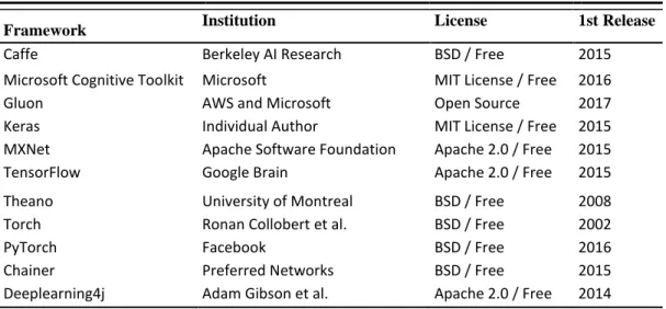
Along with different types of training, algorithms and architecture, we also have different machine learning frameworks (Table 1) and libraries that have made training models easier. These frameworks make complex mathematical functions, training algorithms and statistically modeling available without having to write them on your own. Some provide distributed and parallel processing capabilities, and convenient development and deployment features. Figure 3 shows a graph with various deep learning libraries along with their Github stars from 2015-2018. Github is the largest hosting service provider of source code in the world [25]. Github stars are indicative of how popular a project is on Github. TensorFlow is the most popular DL library.

(31)

31

Table 1. Popular Deep Learning Frameworks and Libraries

Framework Institution License 1st Release

Caffe Berkeley AI Research BSD / Free 2015

Microsoft Cognitive Toolkit Microsoft MIT License / Free 2016

Gluon AWS and Microsoft Open Source 2017

Keras Individual Author MIT License / Free 2015

MXNet Apache Software Foundation Apache 2.0 / Free 2015

TensorFlow Google Brain Apache 2.0 / Free 2015

Theano University of Montreal BSD / Free 2008

Torch Ronan Collobert et al. BSD / Free 2002

PyTorch Facebook BSD / Free 2016

Chainer Preferred Networks BSD / Free 2015

Deeplearning4j Adam Gibson et al. Apache 2.0 / Free 2014

2.2DNN Architectures

Deep neural network consists of several layers of nodes. Different architectures have been developed to solve problems in different domains or use-cases. E.g., CNN is used most of the time in computer vision and image recognition, and RNN is commonly used in time series problems/forecasting. On the other hand, there is no clear winner for general problems like classification as the choice of architecture could depend on multiple factors. Nonetheless [27] evaluated 179 classifiers and concluded that parallel random forest or parRF_t, which is essentially parallel implementation of variation of decision tree, performed the best. Below are three of the most common architectures of deep neural networks.

1. Convolution Neural Network (CNN) 2. Autoencoder

3. Restricted Boltzmann Machine (RBM) 4. Long Short-Term Memory (LSTM)

(32)

32

2.2.1 Convolution Neural Network

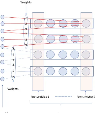
CNN is based on the human visual cortex and is the neural network of choice for computer vision (image recognition). It has been applied to areas such has cancer diagnosis, self-driving cars, etc. As shown in Figure 4a, a CNN consists of a series of convolution and sub-sampling layers followed by a fully connected layer and a normalizing (e.g., softmax function) layer. Figure 4a illustrates the well-known 7 layered LeNet-5 CNN architecture devised by LeCun et al. [28] for digit recognition. The series of multiple convolution layers perform progressively more refined feature extraction at every layer moving from input to output layers. Fully connected layers that perform classification follow the convolution layers. Sub-sampling or pooling layers are often inserted between each convolution layers.

Figure 4a. 7-layer Architecture of CNN for character recognition [28]

CNN’s takes a 2D 𝑛 𝑥 𝑛 pixelated image as an input. Each layer consists of groups of 2D neurons called filters or kernels. Unlike other neural networks, neurons in each feature extraction layers of CNN are not connected to all neurons in the adjacent layers. Instead, they are only connected to the spatially mapped fixed sized and partially overlapping neurons in the previous layer’s input image or feature map. This region in the input is called local receptive field. The lowered number of connections reduces

(33)

33

training time and chances of overfitting. As show in Figure 4b, all neurons in a filter are connected to the same number of neurons in the previous input layer (or feature map) and are constrained to have the same sequence of weights and biases. These factors speed up the learning and reduces the memory requirements for the network. Thus, each neuron in a specific filter looks for the same pattern but in different parts of the input image. Sub-sampling layers reduce the size of the network. In addition, along with local receptive fields and shared weights (within the same filter), it effectively reduces the network’s susceptibility of shifts, scale and distortions of images [29]. Max/mean pooling or local averaging filters are used often to achieve sub-sampling. The final layers of CNN are responsible for the actual classifications, where neurons between the layers are fully connected. Deep CNN can be implemented with multiple series of weight-sharing convolution layers and sub-sampling layers.

(34)

34

The deep nature of the CNN results in high quality representations while maintaining locality, reduced parameters and invariance to minor variations in the input image [30]. In most cases, backpropagation is used solely for training all parameters (weights and biases) in CNN. Here is a brief description of the algorithm. The cost function with respect to individual training example (𝑥, 𝑦) in hidden layers can be defined as [31]:

𝐽(𝑊, 𝑏; 𝑥, 𝑦) =1

2||ℎ𝑤,𝑏(𝑥) − 𝑦||

2₍₃₎

The equation for error term 𝛿 for layer 𝑙 is given by [31]:

𝛿(𝑙) =((𝑊(𝑙))𝑇𝛿(𝑙+1)) . 𝑓′(𝑧(𝑙)) (4)

Where 𝛿(𝑙+1) is the error for (𝑙 + 1)th layer of a network whose cost function is

𝐽(𝑊, 𝑏; 𝑥, 𝑦). 𝑓′_(𝑧(𝑙)₎_{represents the derivate of the activation function.}

𝛻_𝑤(𝑙)𝐽(𝑊, 𝑏; 𝑥, 𝑦) = 𝛿(𝑙+1) (𝑎(𝑙+1))𝑇 (5)

𝛻_𝑏(𝑙)𝐽(𝑊, 𝑏; 𝑥, 𝑦)= 𝛿(

𝑙+1)

(6)

Where 𝑎 is the input, such that 𝑎(1) is the input for 1st layer (i.e., the actual input image) and 𝑎(𝑙) is the input for 𝑙 − 𝑡ℎ layer.

Error for sub-sampling layer is calculated as [31]:

(35)

35

Where 𝑘 represent the filter number in the layer. In the sub-sampling layer, the error has to be cascaded in the opposite direction, e.g., where mean pooling is used, upsample evenly distributes the error to the previous input unit. And finally, here is the gradient w.r.t. feature maps [31]:

𝛻 𝑤_𝑘(𝑙)𝐽(𝑊, 𝑏; 𝑥, 𝑦) =∑(𝑎𝑖 (𝑙)₎ 𝑚 𝑖−1 ∗ 𝑟𝑜𝑡90 (𝛿_𝑘(𝑙+1), 2) (8) 𝛻 𝑏_𝑘(𝑙)𝐽(𝑊, 𝑏; 𝑥, 𝑦)=∑(𝛿𝑘 (𝑙+1) ) 𝑎,𝑏. 𝑎,𝑏 (9)

Where (𝑎_𝑖(𝑙)) ∗ 𝛿_𝑘(𝑙+1)represents the convolution between error and the 𝑖 − 𝑡ℎ

input in the 𝑙 − 𝑡ℎ layer with respect to the 𝑘 − 𝑡ℎ filter.

Algorithm 1 represents a high-level description and flow of the backpropagation algorithm as used in a CNN as it goes through multiple epochs until either the maximum iterations are reached, or the cost function target is met.

In addition to discriminative models such as image recognition, CNN can also be used for generative models such as deconvolving images to make blurry image sharper. [32] achieves this by leveraging Fourier transformation to regularize inversion of the blurred images and denoising. Different implementations of CNN has shown continuous improvement of accuracy in computer vision. The improvements are tested against the same benchmark (ImageNet) to ensure unbiased results.

(36)

36

Algorithm 1: CNN Backpropagation Algorithm Pseudo Code 1:𝐼𝑛𝑖𝑡𝑖𝑎𝑙𝑖𝑧𝑎𝑡𝑖𝑜𝑛𝑤𝑒𝑖𝑔ℎ𝑡𝑠𝑡𝑜𝑟𝑎𝑛𝑑𝑜𝑚𝑙𝑦𝑔𝑒𝑛𝑒𝑟𝑎𝑡𝑒𝑑𝑣𝑎𝑙𝑢𝑒(𝑠𝑚𝑎𝑙𝑙) 2:𝑆𝑒𝑡𝑙𝑒𝑎𝑟𝑛𝑖𝑛𝑔𝑟𝑎𝑡𝑒𝑡𝑜𝑎𝑠𝑚𝑎𝑙𝑙𝑣𝑎𝑙𝑢𝑒(𝑝𝑜𝑠𝑖𝑡𝑖𝑣𝑒) 3:𝐼𝑡𝑒𝑟𝑎𝑡𝑖𝑜𝑛𝑛 = 1; 𝑩𝒆𝒈𝒊𝒏 4: 𝒇𝒐𝒓𝑛 < 𝑚𝑎𝑥𝑖𝑡𝑒𝑟𝑎𝑡𝑖𝑜𝑛𝑂𝑅𝐶𝑜𝑠𝑡𝑓𝑢𝑛𝑐𝑡𝑖𝑜𝑛𝑐𝑟𝑖𝑡𝑒𝑟𝑖𝑎𝑚𝑒𝑡, 𝒅𝒐 5: 𝒇𝒐𝒓𝑖𝑚𝑎𝑔𝑒𝑥1𝑡𝑜𝑥𝑖, 𝒅𝒐 6: 𝑎. 𝐹𝑜𝑟𝑤𝑎𝑟𝑑𝑝𝑟𝑜𝑝𝑎𝑔𝑎𝑡𝑒𝑡ℎ𝑟𝑜𝑢𝑔ℎ 𝑐𝑜𝑛𝑣𝑜𝑙𝑢𝑡𝑖𝑜𝑛, 𝑝𝑜𝑜𝑙𝑖𝑛𝑔𝑎𝑛𝑑𝑡ℎ𝑒𝑛𝑓𝑢𝑙𝑙𝑦𝑐𝑜𝑛𝑛𝑒𝑐𝑡𝑒𝑑𝑙𝑎𝑦𝑒𝑟𝑠 7: 𝑏. 𝐷𝑒𝑟𝑖𝑣𝑒𝐶𝑜𝑠𝑡𝐹𝑢𝑐𝑡𝑖𝑜𝑛𝑣𝑎𝑙𝑢𝑒𝑓𝑜𝑟𝑡ℎ𝑒𝑖𝑚𝑎𝑔𝑒 8: 𝑐. 𝐶𝑎𝑙𝑐𝑢𝑙𝑎𝑡𝑒𝑒𝑟𝑟𝑜𝑟𝑡𝑒𝑟𝑚𝛿(𝑙)𝑤𝑖𝑡ℎ 𝑟𝑒𝑠𝑝𝑒𝑐𝑡𝑡𝑜𝑤𝑒𝑖𝑔ℎ𝑡𝑠𝑓𝑜𝑟𝑒𝑎𝑐ℎ 𝑡𝑦𝑝𝑒𝑜𝑓𝑙𝑎𝑦𝑒𝑟𝑠. 9: 𝑁𝑜𝑡𝑒𝑡ℎ𝑎𝑡𝑡ℎ𝑒𝑒𝑟𝑟𝑜𝑟𝑔𝑒𝑡𝑠𝑝𝑟𝑜𝑝𝑎𝑔𝑎𝑡𝑒𝑑𝑓𝑟𝑜𝑚𝑙𝑎𝑦𝑒𝑟𝑡𝑜𝑙𝑎𝑦𝑒𝑟𝑖𝑛𝑡ℎ𝑒𝑓𝑜𝑙𝑙𝑜𝑤𝑖𝑛𝑔𝑠𝑒𝑞𝑢𝑒𝑛𝑐𝑒 10: 𝑖. 𝑓𝑢𝑙𝑙𝑦𝑐𝑜𝑛𝑛𝑒𝑐𝑡𝑒𝑑𝑙𝑎𝑦𝑒𝑟 11: 𝑖𝑖. 𝑝𝑜𝑜𝑙𝑖𝑛𝑔𝑙𝑎𝑦𝑒𝑟 12: 𝑖𝑖𝑖. 𝑐𝑜𝑛𝑣𝑜𝑙𝑢𝑡𝑖𝑜𝑛𝑙𝑎𝑦𝑒𝑟 13: 𝑑. 𝐶𝑎𝑙𝑐𝑢𝑙𝑎𝑡𝑒𝑔𝑟𝑎𝑑𝑖𝑒𝑛𝑡𝛻_𝑤 𝑘 (𝑙)𝑎𝑛𝑑𝛻_𝑏 𝑘 (𝑙)𝑓𝑜𝑟𝑤𝑒𝑖𝑔ℎ𝑡𝑠𝛻_𝑤 𝑘 (𝑙)𝑎𝑛𝑑𝑏𝑖𝑎𝑠𝑟𝑒𝑠𝑝𝑒𝑐𝑡𝑖𝑣𝑒𝑙𝑦𝑓𝑜𝑟𝑒𝑎𝑐ℎ 𝑙𝑎𝑦𝑒𝑟 14: 𝐺𝑟𝑎𝑑𝑖𝑒𝑛𝑡𝑐𝑎𝑙𝑐𝑢𝑙𝑎𝑡𝑒𝑑𝑖𝑛𝑡ℎ𝑒𝑓𝑜𝑙𝑙𝑜𝑤𝑖𝑛𝑔𝑠𝑒𝑞𝑢𝑒𝑛𝑐𝑒 15: 𝑖. 𝑐𝑜𝑛𝑣𝑜𝑙𝑢𝑡𝑖𝑜𝑛𝑙𝑎𝑦𝑒𝑟 16: 𝑖𝑖. 𝑝𝑜𝑜𝑙𝑖𝑛𝑔𝑙𝑎𝑦𝑒𝑟 17: 𝑖𝑖𝑖. 𝑓𝑢𝑙𝑙𝑦𝑐𝑜𝑛𝑛𝑒𝑐𝑡𝑒𝑑𝑙𝑎𝑦𝑒𝑟 18: 𝑒. 𝑈𝑝𝑑𝑎𝑡𝑒𝑤𝑒𝑖𝑔ℎ𝑡𝑠 19: 𝑤_𝑗𝑖(𝑙) ← 𝑤_𝑗𝑖(𝑙) +∆𝑤_𝑗𝑖(𝑙) 20: 𝑓. 𝑈𝑝𝑑𝑎𝑡𝑒𝑏𝑖𝑎𝑠 21: 𝑏_𝑗(𝑙) ← 𝑏_𝑗(𝑙) +∆𝑏_𝑗(𝑙)

Here are the well-known variation and implementation of the CNN architecture.

1. AlexNet: CNN developed to run on Nvidia parallel computing platform to support GPUs

2. Inception: Deep CNN developed by Google

3. ResNet: Very deep Residual network developed by Microsoft. It won 1st_place

in the ILSVRC 2015 competition on ImageNet dataset.

4. VGG: Very deep CNN developed for large scale image recognition

5. DCGAN: Deep convolutional generative adversarial networks proposed by [33]. It is used in unsupervised learning of hierarchy of feature representations in input objects.

(37)

37

2.2.2 Autoencoder

Autoencoder is a neural network that uses unsupervised algorithm and learns the representation in the input data set for dimensionality reduction and to recreate the original data set. The learning algorithm is based on the implementation of the backpropagation.

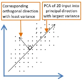
Figure 5. Linear representation of a 2D data input using PCA

Autoencoders extend the idea of principal component analysis (PCA). As shown in Figure 5, a PCA transforms multi-dimensional data into a linear representation. Figure 5 demonstrates how a 2D input data can be reduced to a linear vector using PCA. Autoencoders on the other hand can go further and produce nonlinear representation. PCA determines a set of linear variables in the directions with largest variance. The 𝑝

dimensional input data points are represented as 𝑚 orthogonal directions, such that 𝑚 ≤ 𝑝 and constitutes a lower (i.e., less than 𝑚) dimensional space. The original data points are projected into the principal directions thus omitting information in the corresponding

(38)

38

orthogonal directions. PCA focuses more on the variances rather than covariances and correlations and it looks for the linear function with the most variance [34]. The goal is to determine the direction with the least mean square error, which would then have the least reconstruction error.

Autoencoders use encoder and decoder blocks of non-linear hidden layers to generalize PCA to perform dimensionality reduction and eventual reconstruction of the original data. It uses greedy layer by layer unsupervised pre-training and fine-tuning with backpropagation [35]. Despite using backpropagation, which is mostly used in supervised training, autoencoders are considered unsupervised DNN because they regenerate the input 𝑥(𝑖) itself instead of a different set of target values 𝑦(𝑖), i.e., 𝑦(𝑖) = 𝑥(𝑖). Hinton et al. were able to achieve a near perfect reconstruction of 784-pixel images using autoencoder, proving that it is far better than PCA [36].

While performing dimensionality reduction, autoencoders come up with interesting representations of the input vector in the hidden layer. This is often attributed to the smaller number of nodes in the hidden layer or every second layer of the two-layer blocks. But even if there are higher number of nodes in the hidden layer, a sparsity constraint can be enforced on the hidden units to retain interesting lower dimension representations of the inputs. To achieve sparsity, some nodes are restricted from firing, i.e., the output is set to a value close to zero.

Figure 6 shows single layer feature detector blocks of RBMs used in pre-training, which is followed by unrolling [36]. Unrolling combines the stacks of RBMs to create

(39)

39

the encoder block and then reverses the encoder block to create the decoder section, and finally the network is fine-tuned with backpropagation [36].

Figure 6. Training stages in Autoencoder [36]

Figure 7 illustrates a simplified representation of how autoencoders can reduce the dimension of the input data and learn to recreate it in the output layer. Wang et al. [37] successfully implemented a deep autoencoder with stacks of RBM blocks similar to Figure 6 to achieve better modeling accuracy and efficiency than the proper orthogonal decomposition (POD) method for dimensionality reduction of distributed parameter

(40)

40

systems (DPSs). The equation below describes the average of activation function 𝑎_𝑗(2) of

𝑗𝑡ℎ unit of 2nd layer when the 𝑥𝑡ℎ input activates the neuron [38].

𝜌̂ 𝑗 = 1 𝑚∑ [𝑎𝑗 (2) 𝑚 𝑖=1 𝑥(𝑖) ] (10)

Figure 7. Autoencoder nodes

A sparsity parameter 𝜌is introduced such that 𝜌 is very close to zero, e.g., 0.03

and 𝜌̂ = 𝜌. To ensure that 𝜌̂ = 𝜌, a penalty term 𝐾𝐿(𝜌|| 𝜌̂ )_𝑗 is introduced such that the

Kullback–Leibler (KL) divergence term 𝐾𝐿(𝜌||𝜌̂ )_𝑗 = 0, if 𝜌̂ = 𝜌_𝑗 , else becomes large monotonically as the difference between the two values diverges [38]. Here is the updated cost function [38]:

𝐽𝑠𝑝𝑎𝑟𝑠𝑒(𝑊, 𝑏)= 𝐽(𝑊, 𝑏) + 𝛽 ∑ 𝐾𝐿(𝜌|| 𝜌̂ )𝑗

𝑠2

𝑗=1

(41)

41

Where s2 equals the number of units in 2nd layer and 𝛽 is the parameter than controls sparsity penalty term’s weight.

2.2.3 Restricted Boltzmann Machine (RBM)

Restricted Boltzmann Machine is an artificial neural network where we can apply unsupervised learning algorithm to build non-linear generative models from unlabeled data [39]. The goal is to train the network to increase a function (e.g., product or log) of the probability of vector in the visible units so it can probabilistically reconstruct the input. It learns the probability distribution over its inputs. As shown in Figure 8, RBM is made of two-layer network called the visible layer and the hidden layer. Each unit in the visible layer is connected to all units in the hidden layer and there are no connections between the units in the same layer.

The energy (E) function of the configuration of the visible and hidden units, (v, h) is expressed in the following way [40]:

E(v, h) = − ∑ 𝑎𝑖𝑣𝑖 𝑖 𝜀 𝑣𝑖𝑠𝑖𝑏𝑙𝑒 − ∑ 𝑏𝑗ℎ𝑗 𝑗 𝜀 ℎ𝑖𝑑𝑑𝑒𝑛 − ∑ 𝑣𝑖ℎ𝑗 𝑖,𝑗 𝑤𝑖𝑗 (12)

vi and hj are the vector states of the visible unit i and hidden unit j. ai and bj

represents the bias of visible and hidden units. Wij denotes the weight between the

respective visible and hidden units.

The partition function, Z is represented by the sum of all possible pairs of visible and hidden vectors [40].

(42)

42

Figure 8. Restricted Boltzmann Machine

𝑍 = ∑ 𝑒−𝐸 (𝑣,ℎ)

𝑣,ℎ (13)

The probability of every pair of visible and hidden vectors is given by the following [40].

𝑝(𝑣, ℎ) =1

𝑍𝑒

−𝐸 (𝑣,ℎ) ₍₁₄₎

The probability of a particular visible layer vector is provided by the following [40].

𝑝(𝑣) =1

𝑍∑ 𝑒 −𝐸 (𝑣,ℎ)

ℎ (15)

As you can see from the equations above, the partition function becomes higher with lower energy function value. Thus during the training process, the weights and biases of the network are adjusted to arrive at a lower energy and thus maximize the probability assigned to the training vector. It is mathematically convenient to compute the derivative of the log probability of a training vector.

𝜕 log 𝑝(𝑣) 𝜕𝑤𝑖𝑗

(43)

43

In the equation [40] above 〈vihj〉data and 〈vihj〉model represents the expectations

under the respective distributions.

Thus, the adjustments in the weights can be denoted as follows [40], where ϵ is the learning rate.

∆𝑤𝑖𝑗 = 𝜖(〈𝑣𝑖ℎ𝑗〉𝑑𝑎𝑡𝑎− 〈𝑣𝑖ℎ𝑗〉𝑚𝑜𝑑𝑒𝑙) (17)

2.2.4 Long Short-Term Memory (LSTM)

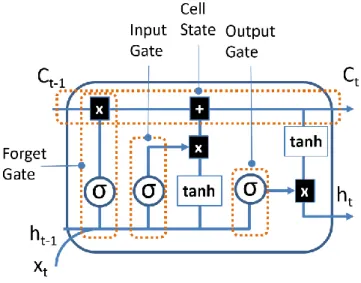
LSTM is an implementation of the Recurrent Neural Network and was first proposed by Hochreiter et al. in 1997 [41]. Unlike the earlier described feed forward network architectures, LSTM can retain knowledge of earlier states and can be trained for work that requires memory or state awareness. LSTM partly addresses a major limitation of RNN, i.e., the problem of vanishing gradients by letting gradients to pass unaltered. As shown in the illustration in Figure 9, LSTM consists of blocks of memory cell state through which signal flows while being regulated by input, forget and output gates. These gates control what is stored, read and written on the cell. LSTM is used by Google, Apple and Amazon in their voice recognition platforms [42].

In Figure 9, 𝐶, 𝑥, ℎ represent cell, input and output values. Subscript 𝑡 denotes time step value, i.e., 𝑡 − 1 is from previous LSTM block (or from time 𝑡 − 1) and

𝑡 denotes current block values. The symbol σ is the sigmoid function and 𝑡𝑎𝑛ℎ is the hyperbolic tangent function. Operator + is the element-wise summation and x is the element-wise multiplication.

(44)

44

Figure 9. LSTM Block with memory cell and gates

The computations of the gates are described in the equations below[41, 43].

𝑓_𝑡= 𝜎(𝑊_𝑓𝑥_𝑡+ 𝑤_𝑓ℎ_𝑡−1+ 𝑏_𝑓) (18)

𝑖_𝑡= 𝜎(𝑊_𝑖𝑥_𝑡+ 𝑤_𝑖ℎ_𝑡−1+ 𝑏_𝑖) (19)

𝑜_𝑡 = 𝜎(𝑊_𝑜𝑥_𝑡+ 𝑤_𝑜ℎ_𝑡−1+ 𝑏_𝑜) (20)

𝑐𝑡 = 𝑓𝑡 ⨂𝑐𝑡−1+ 𝑖𝑡⨂ 𝜎𝑐(𝑊𝑐𝑥𝑡+ 𝑤𝑐ℎ𝑡−1+ 𝑏𝑐) (21)

ℎ𝑡 = 𝑜𝑡 ⨂ 𝜎ℎ(𝑐𝑡) (22)

Where 𝑓, 𝑖, 𝑜 are the forget, input and output gate vectors respectively.

𝑊, 𝑤, 𝑏 𝑎𝑛𝑑 ⨂ represent weights of input, weights of recurrent output, bias and

(45)

45

There is a smaller variation of the LSTM known as gated recurrent units (GRU). GRUs are smaller in size than LSTM as they don’t include the output gate, and can perform better than LSTM on only some simpler datasets[44, 45].

LSTMs recurrent neural networks can keep track of long-term dependencies. Therefore, they are great for learning from sequence input data and building models that rely on context and earlier states. The cell block of LSTM retains pertinent information of previous states. The input, forget and output gates dictates new data going into the cell, what remains in the cell and the cell values used in the calculation of the output of the LSTM block respectively [41, 43]. Naul et al. demonstrated LSTM and GRU based autoencoders for automatic feature extractions [46].

2.2.5 Comparison of DNN Networks

Table 2 provides a compact summary and comparison of the different DNN architectures. The examples of implementations, applications, datasets and DL software frameworks presented in the table are not implied to be exhaustive. In addition, some of the categorization of the network architectures could be implemented in hybrid fashion. E.g., even though RBMs are generative models and their training is considered unsupervised, they can have elements of discriminative model when training is fine-tuned with supervised learning. The table also provides examples of common applications for using different architectures.

(46)

46

Table 2: DNN Network comparison table

Network Type Architecture Network Model Training Type Training Algorithm Implementation Sample Common Application Popular Dataset Sample DL Framework (sample) Fe edf o rwar d N eur al N et wo rk CNN Discrimina tive Supervised Gradient Descent based Backpropagat ion Siamese Network, Deep CNN Image recognition/classif ication MNIST TensorFlow, Caffe, Theano, Torch, Deeplearning4j, Microsoft Cognitive Toolkit, Keras, MXNet, PyTorch Residual Network Discrimina tive Supervised Gradient Descent based Backpropagat ion Deep ResNet; HighwayNet; DenseNet

Image recognition ImageNet TensorFlow,

PyTorch, Keras

Autoencoder Generative Unsupervi sed Backpropagat ion Sparse Autoencoders, Variational Autoencoders Dimensionality Reduction; Encoding MNIST TensorFlow, Deeplearning4j, Keras Adversarial Networks Generative & Discrimina tive Unsupervi sed Backpropagat ion Generative Adversarial Network Generate realistic fake data; Reconstruction of 3D models; Image improvement

CIFAR10 TensorFlow, Keras

RBM Generative with Discrimina tive finetuning Unsupervi sed Gradient Descent based Contrastive divergence Deep Belief Network; Deep Boltzmann Machine Dimensionality Reduction; Feature learning; Topic modeling MNIST TensorFlow, Deeplearning4j, Keras, MXNet, Theano, Torch Recurrent Neural Network LSTM Discrimina tive Supervised Gradient Descent & Backpropagat ion through Time Deep RNN, Gated Recurrent Unit (GRU), Neural Machine Translation (NMT) Natural Language Processing; Language Translation MNIST Stroke Sequence TensorFlow, Caffe, Theano, Torch, Deeplearning4j, Microsoft Cognitive Toolkit, Keras, MXNet, PyTorch Radial Basis Function NN RBF Network Discrimina tive Supervised and Unsupervi sed K-means Clustering; Least Square Function Radial Basis Function NN Function approximation; Time series prediction Fisher's Iris

data set TensorFlow

Kohonen Self Organizing NN Nodes arranged in hexagonal or rectangular grid Generative Unsupervi sed Competitive Learning Kohonen Self Organizing NN Dimensionality Reduction; Optimization problems; Clustering analysis SPAMbase TensorFlow

(47)

47

2.3 Dataset

Access to data is a critical factor for training robust ML models. The explosion of smart devices, sensors, cloud and edge computing have resulted in massive volume, variety and velocity of data. While this has been a tremendous boon to ML, normalizing and sanitizing this data before utilizing them for training is a challenge. The goal of dataset optimization is to reduce the dimensions or the size of the dataset with the intent of improving the accuracy and/or reducing training time, without compromising on the quality. There are several type of dataset optimization methods that are currently in practice.

Dataset optimization including importance sampling has been used to fine-tune the training process and achieve both training speed-up and accuracy improvement. Here are some of the earlier related work.

[47] enhanced variations of stochastic optimization (prox-SMD and prox-SDCA) with importance sampling to reduce the variance resulting in better convergence rate of the training. [48] optimized the training of CNN and RNN with importance sampling by computing an upper bound for the gradient and estimation for the variance reduction.

Dataset and training data in general come with lot of noise that do not contribute to the training process and in some cases hinder training. An effective sampling from the full dataset is a great way to address this concern. [49] showed that the sampling based of word frequency compression and speaker distribution can have a positive impact on training.

(48)

48

2.4 Training Algorithms

The learning algorithm constitutes the main part of Deep Learning. The number of layers differentiates the deep neural network from shallow ones. The higher the number of layers, the deeper it becomes. Each layer can be specialized to detect a specific aspect or feature.

As indicated by Maryam M Jajafabadi et al. [50], in case of image (face) recognitions, first layer can detect edges and the second can detect higher features such as various part of the face, e.g., ears, eyes, etc., and the third layer can go further up the complexity order by even learning facial shapes of various persons. Even though each layer might learn or detect a defined feature, the sequence is not always designed for it, especially in unsupervised learning. These feature extractors in each layer had to be manually programmed prior to the development of training algorithms such as gradient descent. These hand-crafted classifiers didn’t scale for lager dataset or adapt to variation in the dataset. This message was echoed in the 1998 paper [28] by Yann Lecun et al., where they demonstrate that systems with more automatic learning and reduced manually designed heuristics yields far better pattern recognition.

Backpropagation provides representation learning methodology, where raw data can be fed without the need to manually massage it for classifiers, and it will automatically find the representations needed for classification or recognition [15]. The goal of the learning algorithm is to find the optimal values for the weight vectors to solve a class of problem in a domain.

(49)

49

Some of the well-known training algorithms are:

1. Gradient Descent

2. Stochastic Gradient Descent 3. Momentum

4. Levenberg–Marquardt algorithm 5. Backpropagation through time

2.4.1 Gradient Descent

Gradient descent (GD) is the underlying idea in most of machine learning and deep learning algorithms. It is based on the concept of Newton’s Algorithm for finding the roots (or zero value) of a 2D function. To achieve this, we randomly pick a point in the curve and slide to the right or left along the x-axis based on negative or positive value of the derivative or slope of the function at the chosen point until the value of the y-axis, i.e., function or f(x) becomes zero. The same idea is used in gradient descent, where we traverse or descend along a certain path in a multi-dimensional weight space if the cost function keeps decreasing and stop once the error rate ceases to decrease. Newton’s method is prone to getting stuck in local minima if the derivative of the function at the current point is zero. Likewise, this risk is also present when using gradient descent on a non-convex function. In fact, the impact is amplified in the multi-dimensional (each dimension represents a weight variable) and multi-layer landscape of DNN and it result in a sub-optimal set of weights. Cost function is one half the square of the difference between the desired output minus the current output as shown below.

(50)

50

C =1

2(𝑦expected − 𝑦𝑎𝑐𝑡𝑢𝑎𝑙)

2

(23)

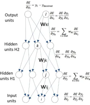
Backpropagation methodology uses gradient descent. In backpropagation, chain rule and partial derivatives are employed to determine error delta for any change in the value of each weight. The individual weights are then adjusted to reduce the cost function after every learning iteration of training data set, resulting in a final multi-dimensional (multi-weight) landscape of weight values [15]. We process through all the samples in the training dataset before applying the updates to the weights. This process is repeated until cost function doesn’t reduce any further.

Figure 10 shows the error derivatives in relation to outputs in each hidden layer, which is the weighted summation of the error derivates in relation to the inputs in the unit in the above layer. E.g., when 𝜕𝐸/𝜕𝑧_𝑘calculated, the partial error derivative with respect to 𝑤𝑗𝑘 to is equal to𝑦𝑗𝜕𝐸/𝜕𝑧𝑘.

(51)

51

2.4.2. Stochastic Gradient Descent

Stochastic Gradient Descent (SGD) is the most common variation and implementation of gradient descent. In gradient descent, we process through all the samples in the training dataset before applying the updates to the weights. While in SGD, updates are applied after running through a minibatch of n number of samples. Since we are updating the weights more frequently in SGD than in GD, we can converge towards global minimum much faster.

2.4.3. Momentum

In the standard SGD, learning rate is used as a fixed multiplier of the gradient to compute step size or update to the weight. This can cause the update to overshoot a potential minima, if the gradient is too steep, or delay the convergence if the gradient is noisy. Using the concept of momentum in physics, the momentum algorithm presents a velocity 𝑣 variable that configured as an exponentially decreasing average of the gradient [51]. This helps prevent costly descent in the wrong direction. In the equation below,

𝛼 ∈ [0,1) is the momentum parameter and 𝜖 is the learning rate.

𝑉𝑒𝑙𝑜𝑐𝑖𝑡𝑦 𝑈𝑝𝑑𝑎𝑡𝑒: 𝑣 ← 𝛼𝑣 − 𝜖𝑔 (24)

𝐴𝑐𝑡𝑢𝑎𝑙 𝑈𝑝𝑑𝑎𝑡𝑒: 𝜃 ← 𝜃 + 𝑣 (25)

2.4.4 Levenberg-Marquardt algorithm

Levenberg-Marquadt algorithm (LMA) is primarily used in solving non-linear least squares problems such as curve fitting. In least squares problems, we try to fit a

(52)

52

given data points with a function with the least amount of sum of the squares of the errors between the actual data points and points in the function. LMA uses a combination of gradient descent and Gauss-Newton method. Gradient descent is employed to reduce the sum of the squared errors by updating the parameters of the function in the direction of the steepest-descent, while the Gauss-Newton method minimizes the error by assuming the function to be locally quadratic and finds the minimum of the quadratic [52].

If the fitting function is denoted by ŷ(t;p) and m data points denoted by (ti,yi), then the squared

error can be written as [52]:

𝑥2(𝒑)=∑ [y(𝑡𝑖)− ŷ(𝑡𝑖;𝐩) 𝜎_𝑦𝑖 ] 2 𝑚 𝑖=1 (26) = (𝑦 − ŷ(𝑝))𝑇_{𝑊 (𝑦 − ŷ(𝑝)) (27)} = 𝑦𝑇_{𝑊𝑦 − 2𝑦}𝑇_{𝑊ŷ + ŷ}𝑇_{𝑊ŷ (28)}

where the measurement error for y (ti), i.e., σyi is the inverse of the weighting matrix Wii.

The gradient descent of the squared error function in relation to the n parameters can be denoted as [52]: ∂ ∂𝐩𝑥 2 _{= 2(𝑦 − ŷ}₍_𝑝₎₎𝑇_𝑊 ∂ ∂𝐩 (𝑦 − ŷ(𝑝)) (29) = 2(𝑦 − ŷ(𝑝))𝑇_{𝑊 [}∂ŷ(𝑝) ∂𝐩 ] (30) = 2(𝑦 ŷ)𝑇_{𝑊 𝐉 (31)}

(53)

53

h_gd = 𝛼 𝐉𝑇𝑊 (𝑦 − ŷ) (32)

where J is the Jacobian matrix of size m x n used in place of the [∂ŷ/ ∂p], and h_gd

is the update in the direction of the steepest gradient descent.

The equation for the Gauss-Newton method update (h_gn) is as follows [52]:

[J𝑇WJ]h_gn = J𝑇W(𝑦 − ŷ) (33)

The Levenberg- Marquardt update [h_lm] is generated by combining gradient descent and Gauss-Newton methods resulting in the equation below [52]:

[J𝑇WJ + λ diag (J𝑇WJ)] hlm= J𝑇W(𝑦 − ŷ) (34)

2.4.5 Backpropagation Through Time

Backpropagation through time (BPTT) is the standard method to train the recurrent neural network. As shown in Figure 2b, the unrolling of RNN in time makes it appears like a feedforward network. But unlike the feedforward network, the unrolled RNN has the same exact set of weight values for each layer and represents the training process in time domain. The backward pass through this time domain network calculates the gradients with respect to specific weights at each layer. It then averages the updates for the same weight at different time increments (or layers) and changes them to ensure the value of weights at each layer continues to stay uniform.