Graph Deep Learning: Methods and Applications

(1)

Washington University in St. Louis Washington University in St. Louis

Washington University Open Scholarship

Engineering and Applied Science Theses &

Dissertations McKelvey School of Engineering

Winter 12-15-2019

Graph Deep Learning: Methods and Applications

Muhan Zhang

Washington University in St. Louis

Follow this and additional works at: https://openscholarship.wustl.edu/eng_etds Part of the Artificial Intelligence and Robotics Commons

Recommended Citation Recommended Citation

Zhang, Muhan, "Graph Deep Learning: Methods and Applications" (2019). Engineering and Applied Science Theses & Dissertations. 504.

https://openscholarship.wustl.edu/eng_etds/504

This Dissertation is brought to you for free and open access by the McKelvey School of Engineering at Washington University Open Scholarship. It has been accepted for inclusion in Engineering and Applied Science Theses &

(2)

WASHINGTON UNIVERSITY IN ST.LOUIS School of Engineering & Applied Science Department of Computer Science and Engineering

Dissertation Examination Committee: Yixin Chen, Chair

Michael Avidan Sanmay Das Roman Garnett

Brendan Juba Yinjie Tang

Graph Deep Learning: Methods and Applications by

Muhan Zhang

A dissertation presented to The Graduate School of Washington University in

partial fulfillment of the requirements for the degree

(3)

(4)

List of Figures

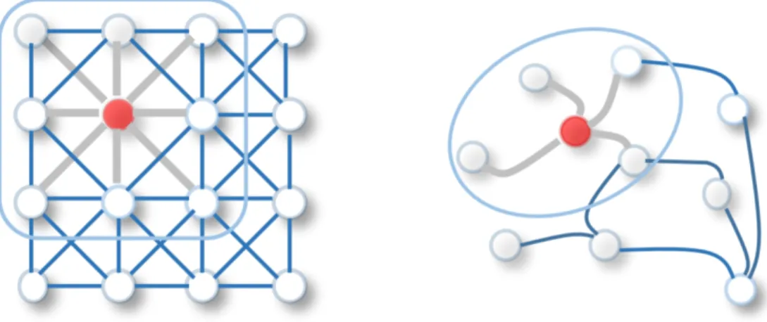
Figure 1.1: 2D convolution (left) vs. graph convolution (right). Graph convolu-tion can be seen as generalizing 2D convoluconvolu-tion on grids to arbitrary structures, where a node’s local receptive field is no longer a fixed-size subgrid, but is defined to be its one-hop neighboring nodes. Figure is from [166]. ... 6 Figure 2.1: A consistent input ordering is crucial for CNNs’ successes on graph

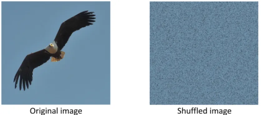
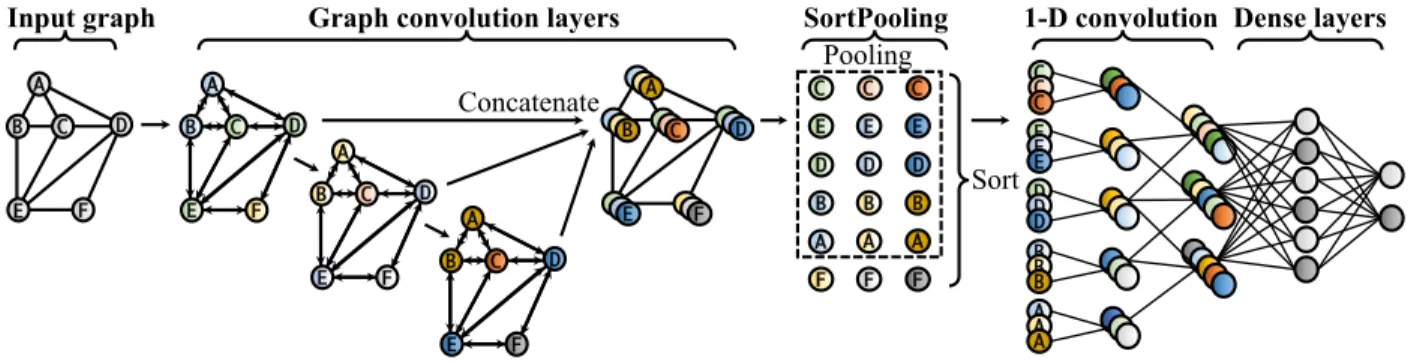
classification. If we randomly shuffle the pixels of the left image, then state-of-the-art convolutional neural networks (CNNs) will fail to recognize it as an eagle. ... 27 Figure 2.2: The overall structure of DGCNN. An input graph is first passed through

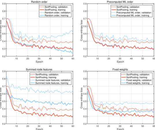
multiple message passing layers where node information is propagated between neighbors. Then the vertex features are sorted and pooled with a SortPooling layer, and passed to 1-D convolutional layers to learn a predictive model... 29 Figure 2.3: Training curves of SortPooling compared with 1) random order, 2)

precomputed WL order, 3) summed node features, and 4) fixed weights. 40 Figure 2.4: Comparison between Gram and HAP. Gram only considers a node’s

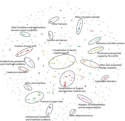
unordered ancestor set to compute its embedding. HAP hierarchically propagate information across the graph. In the bottom-up round, each parent aggregates information from its children. In the top-down round, each child aggregates information from its parents. The final embedding of each node effectively absorbs information from not only its ancestors, but the entire graph (ancestors, descendants, siblings and others). ... 43 Figure 2.5: t-SNE scatterplots of diagnosis code embeddings learned by HAP... 59 Figure 2.6: t-SNE scatterplots of diagnosis code embeddings learned by Gram

(8)

Figure 3.1: The SEAL framework. For each target link, SEAL extracts a local enclosing subgraph around it, and uses a GNN to learn general graph structure features for link prediction. Note that the heuristics listed inside the box are just for illustration – the learned features may be completely different from existing heuristics. ... 68 Figure 3.2: An illustration of our IGMC framework. We extract a local enclosing

subgraph around each training rating, and use a GNN to learn graph patterns that are useful for rating prediction. Note that the features listed inside the box are only for illustration – the learned features can be much more complex. We use the trained GNN to complete other missing entries of the matrix... 86 Figure 4.1: Computations can be represented by DAGs. Note that the left and

right DAGs represent the same computation. ... 105 Figure 4.2: An illustration of the encoding procedure for a neural architecture.

Following a topological ordering, we iteratively compute the hidden state for each node (red) by feeding in its predecessors’ hidden states (blue). This simulates how an input signal goes through the DAG,

with h_v simulating the output signal at node v. ... 108 Figure 4.3: An illustration of the steps for generating a new node. ... 113 Figure 4.4: An example Bayesian network and its encoding. ... 117 Figure 4.5: Top 5 neural architectures found by each model and their true test

accuracies. ... 124 Figure 4.6: Top 5 Bayesian networks found by each model and their BIC scores

(higher the better). ... 125 Figure 4.7: Comparing BO with random search on neural architectures. Left:

average weight-sharing accuracy of the selected points in each iteration. Right: highest weight-sharing accuracy of the selected points over time. 126 Figure 4.8: Comparing BO with random search on Bayesian networks. Left:

aver-age BIC score of the selected points in each iteration. Right: highest BIC score of the selected points over time. ... 127 Figure 4.9: Great circle interpolation starting from a point and returning to itself.

Upper: D-VAE. Lower: S-VAE. ... 127 Figure 4.10: Visualizing a principal 2-D subspace of the latent space. ... 128 Figure A.1: Two bits of change in the string representations can completely change the

(9)

Figure A.2: 2-D visualization of decoded neural architectures. Left: D-VAE. Right: S-VAE... [160] Figure A.3: 2-D visualization of decoded Bayesian networks. Left: D-VAE. Right: S-VAE.[161]

(10)

List of Tables

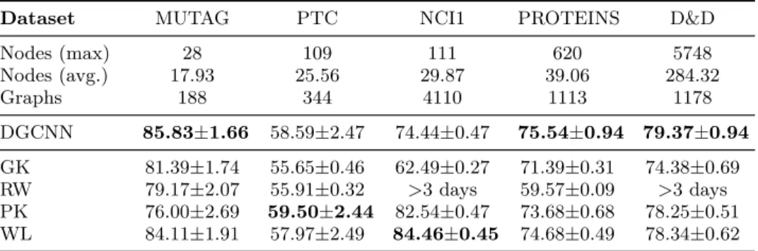
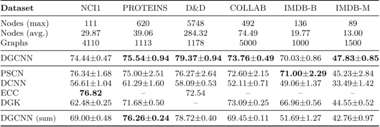
Table 2.1: DGCNN’s comparison with graph kernels. ... 36

Table 2.2: Comparison with other deep learning approaches. ... 38

Table 2.3: Accuracy results on MUTAG for the supplementary experiments... 41

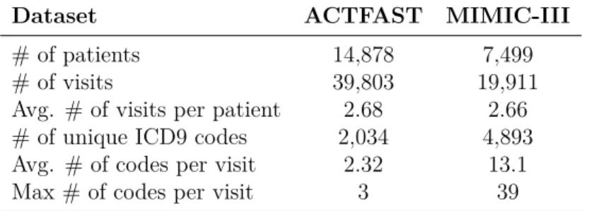
Table 2.4: Statistics of ACTFAST and MIMIC-III datasets. ... 55

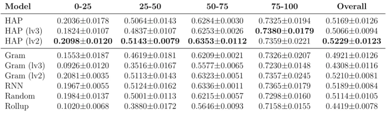
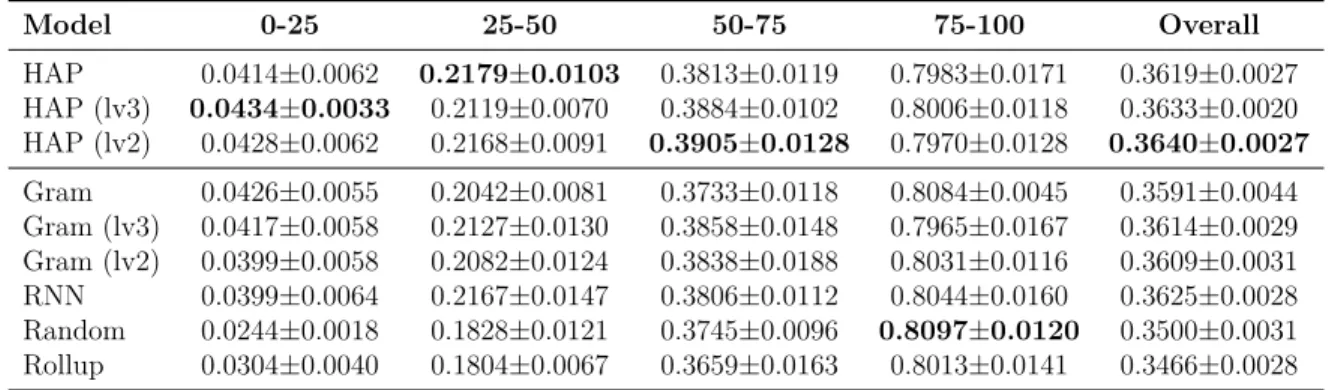
Table 2.5: Grouped and overall Accuracy@5 of sequential procedure prediction on ACTFAST data. ... 57

Table 2.6: Grouped and overall Accuracy@20 of sequential diagnosis prediction on MIMIC-III data. ... 58

Table 3.1: Popular heuristics for link prediction, see [96] for details... 65

Table 3.2: Comparing SEAL with heuristic methods (AUC). ... 80

Table 3.3: Comparing SEAL with latent feature methods (AUC)... 80

Table 3.4: Inference time of SEAL. ... 81

Table 3.5: Comparing SEAL with network embedding methods (AUC) on larger networks, OOM: out of memory). ... 82

Table 3.6: Statistics of each dataset... 94

Table 3.7: RMSE test results on Flixster, Douban and YahooMusic. ... 95

Table 3.8: RMSE test results on MovieLens-100K. ... 96

Table 3.9: RMSE test results on MovieLens-1M. ... 97

Table 3.10: RMSE of transferring models trained on ML-100K to Flixster, Douban and YahooMusic. ... 97

Table 4.1: Reconstruction accuracy, prior validity, uniqueness and novelty (%). .. 122

(11)

(12)

Acknowledgments

First and foremost, I would like to express my deepest gratitude to my advisor, Prof. Yixin Chen, for his guidance, advice and support throughout my PhD study. Thanks to his broad research interest, I got in touch with various interesting problems including link prediction, recommender systems, graph classification, graph neural networks, metabolic networks, time series prediction and so on. From these topics I gradually built up my research interest on graphs, and finally decided to give this dissertation on graph deep learning. I am grateful for all the collaboration opportunities with other departments that he gave to me too. Through interdisciplinary research, I got to know many fascinating real-world applications of machine learning and data mining, which greatly broadened my interest and horizon. I also enjoy talking with him a lot for his wisdom and sense of humor, and always get valuable inspirations and innovative ideas from him. The research skills I learned from him will be invaluable to me in my future career.

I would also like to thank the rest of my committee, Professors Michael Avidan, Sanmay Das, Roman Garnett, Brendan Juba, and Yinjie Tang, for their helpful suggestions to the dissertation. Furthermore, I would like to thank Prof. Avidan for hosting our ACTFAST meetings and pushing the project forward with his great enthusiasm for AI and healthcare. I would like to thank Prof. Das, Prof. Garnett and Prof. Juba for teaching those wonderful

(13)

enjoyed. I am also grateful for the discussions, help and encouragement they provided for my research. I would like to thank Prof. Yinjie Tang for his continuous trust on me, including inviting me to give talks to his class and collaborating on metabolic networks etc.

I would like to thank Anand Bhaskar, Wenlin Chen, Aude Hofleitner, Cheng Ju, Joy Zhang and Zhe Feng for their help during my internship at Facebook. I really enjoyed the time being together with them. Working with them lets me know what excellent researchers do in industry. I would like to thank my collaborators: Zhicheng Cui, Shali Jiang, Christopher R. King, Marion Neumann, Tolutola Oyetunde, for the inspiring discussions, fantastic collaborations, and great teamwork. I would like to thank my friends at WashU: Haipeng Dai, Zehao Dong, Yujie He, Zhiyang Huang, Zhuoshu Li, Haoran Li, Xiaoxin Liu, Chen Liu, Junjie Liu, Yehan Ma, Gustavo Malkomes, Wei Tang, Zhihao Xia, Hao Yan, Hang Yan, Yajie Yan, Jinghan Yang, Mingquan Yuan, Zhen Zhang, Kai Zhou, Liang Zhou, Maede Zolanvari and all others who are not listed here for all the great time and fun we had together.

I would like to thank my father Hongliang Zhang and mother Yanling Sun for their eternal love. They cultivated my interest in computer since I was a child. I still remember how I was attracted by the first computer bought by my father when I was three.

Finally, I would like to thank my beloved wife, Liran Wang, who, regardless of successes or failures, has always accompanied and trusted me. With you, I am not afraid of even the deepest dark, because you are my light.

Muhan Zhang

Washington University in Saint Louis December 2019

(14)

(15)

ABSTRACT OF THE DISSERTATION Graph Deep Learning: Methods and Applications

by Muhan Zhang

Doctor of Philosophy in Computer Science Washington University in St. Louis, 2019

Professor Yixin Chen, Chair

The past few years have seen the growing prevalence of deep neural networks on various application domains including image processing, computer vision, speech recognition, machine translation, self-driving cars, game playing, social networks, bioinformatics, and healthcare etc. Due to the broad applications and strong performance, deep learning, a subfield of machine learning and artificial intelligence, is changing everyone’s life.

Graph learning has been another hot field among the machine learning and data mining communities, which learns knowledge from graph-structured data. Examples of graph learning range from social network analysis such as community detection and link prediction, to relational machine learning such as knowledge graph completion and recommender systems, to mutli-graph tasks such as graph classification and graph generation etc.

An emerging new field, graph deep learning, aims at applying deep learning to graphs. To deal with graph-structured data, graph neural networks (GNNs) are invented in recent years which directly take graphs as input and output graph/node representations. Although GNNs have shown superior performance than traditional methods in tasks such as semi-supervised node classification, there still exist a wide range of other important graph learning problems

(16)

where either GNNs’ applicabilities have not been explored or GNNs only have less satisfying performance.

In this dissertation, we dive deeper into the field of graph deep learning. By developing new algorithms, architectures and theories, we push graph neural networks’ boundaries to a much wider range of graph learning problems. The problems we have explored include: 1) graph classification; 2) medical ontology embedding; 3) link prediction; 4) recommender systems; 5) graph generation; and 6) graph structure optimization.

We first focus on two graph representation learning problems: graph classification and medical ontology embedding. For graph classification, we develop a novel deep GNN architecture which aggregates node features through a novel SortPooling layer that replaces the simple summing used in previous works. We demonstrate its state-of-the-art graph classification performance on benchmark datasets. For medical ontology embedding, we propose a novel hierarchical attention propagation model, which uses attention mechanism to learn embeddings of medical concepts from hierarchically-structured medical ontologies such as ICD-9 and CCS. We validate the learned embeddings on sequential procedure/diagnosis prediction tasks with real patient data.

Then we investigate GNNs’ potential for predicting relations, specifically link prediction and recommender systems. For link prediction, we first develop a theory unifying various traditional link prediction heuristics, and then design a framework to automatically learn suitable heuristics from a given network based on GNNs. Our model shows unprecedented strong link prediction performance, significantly outperforming all traditional methods. For recommender systems, we propose a novel graph-based matrix completion model, which uses a GNN to learn graph structure features from the bipartite graph formed by user and item interactions. Our model not only outperforms various matrix completion baselines, but

(17)

also demonstrates excellent transfer learning ability – a model trained on MovieLens can be directly used to predict Douban movie ratings with high performance.

Finally, we explore GNNs’ applicability to graph generation and graph structure optimization. We focus on a specific type of graphs which usually carry computations on them, namely directed acyclic graphs (DAGs). We develop a variational autoencoder (VAE) for DAGs and prove that it can injectively map computations into a latent space. This injectivity allows us to perform optimization in the continuous latent space instead of the original discrete structure space. We then apply our VAE to two types of DAGs, neural network architectures and Bayesian networks. Experiments show that our model not only generates novel and valid DAGs, but also finds high-quality neural architectures and Bayesian networks through performing Bayesian optimization in its latent space.

(18)

Chapter 1 Introduction

1.1 Graph Deep Learning

Deep learning is changing everyone’s life. One important reason for the superior performance of deep learning over traditional algorithms is that deep learning integrates feature extraction into the model learning itself, i.e., raw input signals (such as image pixels or audio waveforms) are directly fed into the model without performing feature engineering beforehand. Such an end-to-end procedure greatly improves the quality of the extracted features.

Conventional neural network architectures, such as feed-forward neural networks (FFNN), convolutional neural networks (CNNs) and recurrent neural networks (RNNs), require input signals to be represented in fixed-size tensor forms, where each element of a tensor corresponds to a fixed raw input dimension. This way, neural network layers are able to hierarchically extract features and learn patterns from the data. Although achieving great successes on various data types, these conventional neural networks cannot directly be applied to graphs.

(19)

Unlike images, graph-structured data do not have a tensor representation that can be readily read by conventional neural networks, which has limited deep learning’s use cases for graphs. Graph-structured data are abundant in the real world, e.g., social networks, citation networks, biological networks, molecular structures, power grids, knowledge graphs, etc. Furthermore, graph is also an important subject in machine learning, since many machine learning models, such as neural networks and Bayesian networks, are realized as computations on graphs. There exist a wide range of learning problems related to graphs, such as semi-supervised node classification, graph classification, link prediction, community detection, graph clustering, graph generation, network embedding, etc. Due to the abundance of graph data and graph learning problems, it is very important to study how to learn from graphs.

Graph learning is a challenging problem. Firstly, the number of nodes in a graph can be variable, which poses a great challenge for traditional machine learning models that can only take fixed-size input. Secondly, graphs have the isomorphism problem, meaning that the same graph can have factorially many different expressions by simply permuting the nodes, which brings additional challenges to distinguishing graphs. Thirdly, the graph topology contains rich information important for the learning tasks, yet is extremely hard to extract and learn. All these difficulties make graph learning special and different from traditional learning tasks in regular domains.

Because of the special characteristics of graphs, traditional graph learning methods typically rely on predefined structural features such as node degrees, paths, walks, subtrees, frequent subgraphs, etc., and then apply standard machine learning algorithms on the extracted features. Such a two-step procedure separates feature extraction from model learning, which is against deep learning’s end-to-end training principle, thus often having less expressive power. Another way is to use graph kernels [15, 59, 85, 116, 142, 159], which compute

(20)

some positive semidefinite graph similarity measures so that kernel machines such as SVM become feasible for some graph learning tasks. However, graph kernels introduce several new problems. Firstly, computing and storing the kernel matrices require at least quadratic time and space complexity w.r.t. the number of graphs, which is often infeasible for large-scale problems in practice. Secondly, the design of graph kernels is often by heuristics. There is no principled way to measure graph similarities, introducing the need to carefully design different graph kernels for different datasets. Thirdly, graph kernels usually lack the ability to learn representations of graphs, which limits their use cases to only a small range of problems such as graph classification.

To better learn from graphs, graph deep learning aims at leveraging the superior feature learning ability of deep learning for graphs. Since conventional neural networks such as CNNs and RNNs do not work,graph neural networks (GNNs), a new type of neural networks designed particularly for graphs, have recently been proposed [7, 18, 39, 43, 77, 94, 121, 136]. GNNs iteratively pass messages between each node and its neighbors in order to extract local substructure features around nodes. Then, an aggregation operation such as summing is applied to all nodes to get a graph-level feature vector. GNNs are parametric models, thus avoiding the need to compute and store kernel matrices. The learnable parameters in the message passing and aggregation layers equip GNNs with excellent graph representation learning abilities and great flexibility for different graphs. GNNs also enable end-to-end training. Because of these advantages, GNNs gain great popularity in a short time, achieving state-of-the-art performance on semi-supervised node classification [77], network embedding [57], etc.

Despite the success of GNNs in certain problems, as a new tool, GNNs still either do not have satisfying performance or do not find applicabilities in many other important graph learning problems, mainly due to the immature architectures and the shallow understandings people

(21)

have for GNNs. In this dissertation, with a series of innovations in algorithms, architectures and theories, we explore GNNs’ potential and limits in three general fields, namely graph representation learning, relation prediction, and graph structure optimization. We first focus on graph representation learning (Chapter 2), the goal of which is to learn representations for graphs or nodes within a graph. Leveraging innovative GNN architectures and designs, we achieve state-of-the-art results for two graph representation learning tasks, namely graph classification and medical ontology embedding. The second field we explore is using GNNs to predict relations (Chapter 3), e.g., predicting links in social networks and recommending items to users. We show that by extracting local enclosing subgraphs around relations, we are able to automatically learn general graph structure features useful for relation prediction based on GNNs instead of using predefined heuristics. The last field we explore is using GNNs to generate and optimize graph structures (Chapter 4). For this problem, we train a GNN-based variational autoencoder (VAE) for directed acyclic graphs (DAGs), and optimize their structures in the VAE’s latent space based on Bayesian optimization. Our model not only generates valid and novel DAG structures, but also provides promising directions to two important DAG structure optimization problems: neural architecture search (NAS) and Bayesian network structure learning (BNSL).

In the remaining part of this chapter, we review the development history of GNNs and introduce the basics of GNNs, which serve as preliminaries for the following chapters of the dissertation.

1.2 A Brief History of Graph Neural Networks

The earliest graph neural networks can date back to Gori et al. (2005) [55] and Scarselli et al. (2009) [136]. These early attempts use recurrent architectures to learn a target node’s

(22)

representation by iteratively propagating neighbor information until reaching a stable fixed point, which is computationally very expensive. Recently, encouraged by the success of CNNs in computer vision, a great number of approaches have been developed in parallel that generalize the notion of convolution from images to graph data, namely graph convolutions. Based on which domain the convolution operation is performed in, these graph convolution approaches can be categorized into spectral-based approaches and spatial-based approaches. The first remarkable spectral-based method was developed by Bruna et al. (2013) [18], which developed a graph convolution operation based on the spectral graph theory, where learnable filters are applied to a graph’s frequency modes computed by graph Fourier transform [135]. From then on, many approximations of spectral-based graph convolution are proposed [39, 60, 77], which either greatly reduce the computation complexity or make the convolution filters localized. For example, Defferrard et al. [39] parameterize the spectral filters as Chebyshev polynomials of eigenvalues, which achieves both efficient and localized filters. One limitation of the above spectral formulations is that they rely on the fixed spectrum of the graph Laplacian, thus are suitable only for graphs with a single structure (but varying signals on vertices).

Spatial-based graph convolutions, on the contrary, are not restricted to a fixed graph structure. To extract local features, several works independently propose to propagate messages between neighboring vertices, inheriting the ideas from early GNNs [136]. Duvenaud et al. [43] propose differentiable Neural Graph Fingerprints, which propagate features between 1-hop neighbors to simulate the traditional circular fingerprint for molecules. Atwood et al. [7] propose Diffusion-CNN, which propagates neighbors with different hops to the center using different weights. Later, Kipf and Welling (2016) [77] develop a first-order approximation for the spectral convolution of [39] which also simplifies to propagation between neighboring vertices. Niepert et al. [121] propose another way of spatial graph convolution by extracting

(23)

Figure 1.1: 2D convolution (left) vs. graph convolution (right). Graph convolution can be seen as generalizing 2D convolution on grids to arbitrary structures, where a node’s local receptive field is no longer a fixed-size subgrid, but is defined to be its one-hop neighboring nodes. Figure is from [166].

fixed-sized local patches from nodes’ neighborhoods and linearizing these patches with graph labeling methods and graph canonization tools. Figure 1.1 illustrates the similarity and difference between 2D image convolution and spatial graph convolution. Compared to spectral approaches, spatial graph convolutions are more flexible, easier to implement, and largely reduce the computation complexity. Therefore, they have become the mainstream graph convolution approaches used in graph neural networks. In the remaining part of the dissertation, without special notations, graph neural networks all refer to those using spatial approaches.

1.3 Graph Neural Networks Basics

Graph neural networks (GNNs) have many independently developed formulations [18, 35, 39, 43, 94, 136], most of which can be unified into a message passing framework [53]. Given an undirected graphGwith node features x_v (a row vector), the forward pass of a GNN typically contains two phases: a message passing phase (a.k.a. graph convolution) used to extract

(24)

local substructure features around nodes, and an aggregation phase (a.k.a. readout, graph pooling, etc.) used to summarize individual node features into a graph-level feature vector. We will consistently use this message passing form to describe our graph neural networks, but will discuss graph neural networks’ other formulations in the next section. We give a brief introduction to the basics of message passing graph neural networks here for readers who want to skip the next section.

The message passing (graph convolution) phase runs for T iterations and involves message functions Mt and vertex update functionsUt. At each message passing step, vertex hidden

states zt

v are updated based on messages mtv according to: mt+1_v = X u∈Γ(v) Mt(ztv,ztu), (1.1) zt+1_v =Ut(ztv,m t+1 v ), (1.2)

where Γ(v) denotes the set of neighbors ofv in graph G, Mt and Ut are both differentiable

functions with learnable parameters. We omit edge features for simplicity, as edge features are often unavailable. For z0

v, we can let them be the initial node features xv.

The message passing form above has many explanations such as first-order approximation of graph Fourier Transform [39, 77], differentiable approximation of neural graph fingerprints [43], CNN’s generalization from regular grids to graphs [121], etc. However, it also has a straightforward explanation as follows: each step of message passing propagates each node’s 1-hop neighbors’ information to itself, thus summarizing the local substructure patterns around individual nodes; multiple steps of such propagations summarize multi-hop neighborhood information around nodes.

(25)

The message passing can be seen as a convolutional operator applied on nodes to extract local features, similar to what a convolutional layer in traditional CNNs does for each pixel. Most existing graph neural networks can be incorporated into this message passing framework. The differences lie in the unique designs of MtandUtin different works. For example, Mtcan

be as simple as a sum/mean [43] or concatenation [121], or use advanced neural architectures such as the attention mechanism [158] and RNNs [57]. The update functionUt can also range

from a single linear layer to multi-layer perceptrons (MLPs) [179] and GRUs [94, 185], etc. With the extracted hidden states of nodes, we can use them for node-level tasks such as semi-supervised node classification and node embedding. However, we still need to get a graph feature vector for doing graph-level tasks such as graph classification and graph generation. The aggregation phase does this job by:

zG =R({zvT |v ∈G}), (1.3)

where R is a readout (pooling) function that is invariant to permutations of nodes in order for GNNs to be invariant to graph isomorphism. Most previous GNN formulations use a simple summing/averaging over the final node states [7, 35, 43, 94]. We will discuss the disadvantages of using such an averaging operation in the second chapter.

1.4 A Categorization of Graph Neural Networks

In this section, we give a categorization of graph neural networks with respect to the problems they are addressing, and put our own work into the literature. In each categorization, we introduce the most representative works, including their motivations, formulations, and advantages/disadvantages, etc.

(26)

There are mainly three types of problems that all graph neural networks are addressing: node-level tasks, graph-node-level tasks, and edge-node-level tasks. Node-node-level tasks include all node-related graph learning problems, such as semi-supervised node classification [77], network embedding [57], node clustering [162], etc. In graph-level tasks, representations of the entire graphs are learned to allow graph classification [173, 184], graph regression, graph generation [185], etc. In edge-level tasks, representations of edges are learned to enable link prediction [78, 181] or learning recommender systems [berg2017graph, 113, 180], etc., where the task is to predict existence of edges or values of edges.

1.4.1 GNNs for node-level tasks

In node-level tasks, there is typically only one large graph (network) given, and the task is to learn representations for individual nodes of the graph so that downstream node-level tasks can be performed. The node representations can be either learned in a semi-supervised way (i.e., train on some given node labels in an end-to-end way), or in an unsupervised way (i.e., node labels are unknown, and the training is performed by minimizing some auxiliary loss such as reconstructing the graph). Currently, node-level tasks are still the most popular tasks for graph neural networks due to their wide applicabilities in network analysis.

The first graph neural network for learning node states of general graphs is the Graph Neural Network1 _{model, which uses a contractive mapping to recurrently find steady states of nodes}

[136]. However, to ensure convergence, the parameters of the recurrent function has to be constrained via a penalty term on the Jacobian matrix. The repeated use of contractive mapping to find the steady states also poses efficiency problems to practical applications.

1_{It is also where the name GNN comes from. Note that, however, people now use GNN to refer to any}

(27)

Gated Graph Neural Network (GGNN) [94] uses a Gated Recurrent Unit (GRU) [26] as the recurrent function and also no longer requires finding steady states of nodes. Instead, the recurrence is reduced to a fixed number of steps. A node hidden state is updated with

zt+1_v = GRU(zt_v, X

u∈Γ(v)

Wzt_u). (1.4)

GGNN uses the same GRU parameters across different steps (layers), which is different from most GNNs that use different weight parameters across different layers. The advantage is that the recurrent unit, GRU, has the ability to learn to forget and keep information from previous steps, which could benefit long-range node propagations in graphs with large diameters. GGNN is designed for undirected graphs, where the message passing is performed simulateneously for all nodes for multiple rounds. In Chapter 4, we will introduce our work on training a variational autoencoder for directed acyclic graphs (DAGs), where we also leverage a GRU as the node update function yet only need to propagate once for each node following a topological order of nodes.

Instead of using the same recurrent unit for different layers, the majority of graph neural networks use convolutional operators with different parameters for different layers, which is inspired by convolutional neural networks (CNNs) for images. The earliest convolutional neural networks for graphs define convolutions in the spectral domain. Based on the theories on graph signal processing [135, 144], the spectrum of a graph is given by the eigenvalues of the normalized Laplacian matrix of the graph:

(28)

where Λ is the diagonal matrix of the eigenvalues, U is the matrix of the corresponding eigenvectors, andL=I−D−12AD−

1

2 is the normalized Laplacian matrix withA∈ {0,1}n×n

denoting the adjacency matrix and D denoting the diagonal degree matrix of the graph. The graph Fourier transform to a signal on nodes x∈_Rn _{is defined as:}

F(x) =U>x, (1.6) and the inverse graph Fourier transform is defined as:

F−1(ˆx) =Uxˆ, (1.7) where ˆx is the spectral-domain signal resulted from the graph Fourier transform. The graph Fourier transform projects the graph signal xinto an orthogonal space formed by the eigenvectors of the normalized graph Laplacian matrix. In this spectral domain, we can define graph convolution as the element-wise (Hadamard) product of a filter F(g) and the transformed signal F(x), after which we can inversely transform the result signal back to the spatial domain:

x∗Gg:=F−1(F(x)F(g))

=U(U>xU>g). (1.8) If we define g_θ = diag(U>g), then the spectral graph convolution is equivalent to:

x∗Ggθ =UgθU

(29)

All spectral-based graph convolutional neural networks follow this definition and adopt different filters g_θ. The earliest work Spectral Convolutional Neural Network (Spectral-CNN) [18] lets g_θ be a diagonal matrix of learnable parameters, and considers multiple channels of graph signals. Let Θt_i,j be the filter between the ith _{channel of layer} _t_{+ 1 and the} _jth _channel

of layert, the graph convolution layer t is defined as:

Zt+1_:,j =f(

ct

X

i=1

UΘt_i,jU>Zt_:,i), (1.10) where Zt_:,i ∈_Rn×1 _{denotes the} _ith _{channel of the graph signal} _Zt_∈

Rn×ct in the tth layer, and ct is the number of channels in the tth layer. One great limitation of Spectral-CNN is its

O(n3) computation complexity with respect to the number of nodes n, due to the expensive eigen-decomposition.

Later, two follow-up works, ChebNet [39] and GCN [77] reduce the complexity from O(n3₎

to O(m) (m denotes the number of edges) by making simplifications and approximations to (1.10).

Chebyshev Spectral CNN (ChebNet) [39] makes an approximation to g_θ by using Chebyshev polynomials of the diagonal matrix of eigenvalues:

g_θ =

K−1

X

k=0

θiTk( ˆΛ), where ˆΛ= 2Λ/λmax−I. (1.11)

The Chebyshev polynomials can be recursively computed by:

(30)

with T0(x) = 1 andT1(x) =x. Then, the original spectral graph convolution (1.9) can be written as: x∗Ggθ =U( K−1 X k=0 θiTk( ˆΛ))U>x (1.13) = K−1 X k=0 θiTk( ˆL)x, (1.14)

where ˆL = 2L/λmax−I. It is proved that (Lk)i,j = 0 for nodes i and j with dG(i, j) > K,

where dG(i, j) denotes the shortest path length between i, j. Consequently, one advantage

of ChebNet compared to Spectral-CNN is its localized convolution filters by restricting the order of the Chebyshev polynomials K. In contrast, the filters in (1.10) are global, meaning that even signals from distant nodes will contribute to the convolution result of a center node. This contradicts with the principle of traditional CNNs for images which leverage localized filters to learn translation invariant features. Thus, ChebNet is more like CNNs than Spectral-CNN.

However, both ChebNet and Spectral-CNN have another limitation – they only work on a single graph structure. This is because the graph Laplacian matrix they rely on is dependent on the global graph structure – any perturbation to the graph structure can result in a change of the eigenbasis and eigenvalues. This has no influence on node-level and edge-level tasks with a single large graph structure given. However, it will pose problems for graph-level tasks, since the learned structure-dependent filters cannot be applied to graphs with different structures.

Instead of defining graph convolutions in the spectral domain,spatial methodsdefine graph convolutions in the spatial domain (nodes’ spatial relations with other nodes). Spatial-based graph convolutions are motivated directly by traditional CNNs on images where a center

(31)

around it. Spatial-based GNNs similarly convolve a center node state with its neighbors’ states to get an the updated representation of the center node.

Spatial methods are not restricted to a single graph structure, since all convolutions are done locally within a node’s neighborhood without using the global graph structure. Thus, spatial methods can not only be applied to node-level and edge-level tasks, but also graph-level tasks.

The most popular spatial-based graph neural network is the Graph Convolutional Network (GCN) model [77]. Its convolution form is derived by making a first-order approximation of the ChebNet (1.13). In particular, by using order K = 1 and assuming λmax= 2, GCN

simplifies (1.13) to x∗Ggθ =θ0x−θ1D− 1 2AD− 1 2x. (1.15)

Then, GCN makes a further simplification by assuming θ0 = −θ1 := θ, which effectively

reduces the number of parameters to only 1 between every input and output channel. The single-channel graph convolution then becomes:

x∗Ggθ =θ(I+D

−1₂_AD−1₂₎_x_. _(1.16)

And the multi-channel form of GCN can be written into a matrix multiplication form as follows:

Zt+1 =f( ˆAZtΘ), (1.17) where ˆA:=I+D−12AD−

1

2 andfis an activation function. However, using ˆA=I+D− 1 2AD−

1 2

(32)

might cause numerical instabilities. In this regard, GCN uses a renormalization trick which replaces ˆA with ˜D−

1 2_A˜_D˜−

1

2 _{where ˜}_A _:= _A₊_I _{and ˜}_D _{is a diagonal degree matrix of ˜}_A

( ˜Dii =PjA˜ij).

If we look at individual rows zi of Z, we can rewrite (1.17) into: z0_i =f( 1 ˜ Dii y_i+ X j∈Γ(i) 1 q ˜ DiiD˜jj y_j), (1.18)

where Γ(i) denotes the neighbor set of node i, and y_j := Θ>zj. As we can see, the GCN

graph convolution reduces to a weighted sum of the transformed center node state y_i and neighbor node states y_j, j ∈Γ(i), which is in a spatial-based graph convolution form. GCN establishes a relationship between spectral methods and spatial methods.

Diffusion Convolutional Neural Network (DCNN) [7] is another early spatial-based GNN. It treats graph convolutions as a diffusion process. It uses a probability transition matrix

P=D−1A to propagate neighbor states from different hops:

Z(k) =f(W(k)PkX), (1.19) where the final node representations are given by the concatenation of Z(1)_,_Z(2)_{, . . . ,}_Z(K)

. Using a diffusion matrix P automatically decreases the contribution of faraway nodes to the center node. In contrast to GCN [77], nodes more than one hop away from the center node directly propagate their states to the center instead of propagating to the center through multiple layers of graph convolution.

In the previous section, we have briefly introduced message passing neural networks (MPNN) [53], which is a uniform framework for spatial-based GNNs. The complete form of a message

(33)

passing function is given by mt+1_v = X u∈Γ(v) Mt(ztv,z t u,x e vu), (1.20) zt+1_v =Ut(ztv,m t+1 v ), (1.21) wherexe

vuis the edge feature between nodesv,u,Mtis the message function used to aggregate

neighboring node states into a message mv, and Ut is the update function used to update

center node v’s state zv based on the message mv. Edge features are not always available

in graph datasets, thus are often ignored in other works, and are more usually handled in different formulations when edge features are discrete and countable which will be discussed in more details in Section 3.2.

Graph Isomorphism Network (GIN) [168] studies the representative power of message passing networks and finds that message passing networks can be at most as powerful as the Weisfeiler-Lehman algorithm [165] by adding an irrational weight t+1 _{in the update function. It uses a}

graph convolution form as follows:

zt+1_v =f((1 +t+1)zt_v+ X

u∈Γ(v)

Wtzt_u), (1.22)

where the irrational number t+1 _{distinguishes the center node from its neighbors when they}

are assembled together, thus is able to injectively encode the rooted depth-1 subtree of the center node, the same as how the Weisfeiler-Lehman algorithm color nodes (it also uses a perfect hashing function to give unique colors to unique rooted subtree patterns). The Weisfeiler-Lehman algorithm is a powerful tool for distinguishing different graphs, and a promising direction towards efficiently solving the hard graph isomorphism (GI) problem. GIN theoretically shows the graph neural networks can be as powerful as Weisfeiler-Lehman

(34)

algorithm which demonstrates the representative power of GNNs. In practice, GIN lets (t+1)

be a learnable parameter that is trained together with other parameters.

Graph Attention Network (GAT) [158] does not assume identical contributions of neighboring nodes like previous works such as GCN [77] and GIN [168]. Instead, it leverages an attention mechanism to learn the contribution of each neighboring node to the center node. GAT’s graph convolution form is defined as:

zt+1_v =f( X

u∈Γ(v)∪v

αvuWtztu), (1.23)

where the attention weight αvu is given by:

αvu = softmax[g(a>concat(Wtztv,W t_zt

u))], (1.24)

where g is a LeakyReLU activation function and a is a vector of parameters that transforms concatenated node states into a scalar raw weight. And the softmax operation calculates normalized weights so that P

u∈Γ(v)∪vαvu= 1. Multi-head attention can be further used to

increase the model capacity. GAT shows improvements over GCN in node classification tasks. Right now, we have discussed many representative graph neural networks for node-level tasks, mainly in the categories of spectral-based approaches and spatial-based approaches. In Section 2.2, we will discuss our contribution on medical ontology embedding which falls into node-level tasks. We propose a Hierarchical Attention Propagation (HAP) method to learn embeddings of node concepts in a medical ontology such as ICD-9. Our HAP adopts an attention mechanism like GAT, but uses a different propagation order to deal with the special structure of hierarchical medical ontologies. In Section 2.1, we will discuss our contribution to a graph-level task, graph classification, where the node representation learning parts use a

(35)

1.4.2 GNNs for graph-level tasks

GNNs for graph-level tasks are generally less studied than GNNs for node-level tasks. However, node-level GNNs are essential preliminary steps for a successful graph-level GNN. Concretely speaking, a graph-level GNN is typically composed of a node-level GNN used to extract individual node feature states and a pooling layer used to summarize node states into a graph representation. Our main contribution for graph classification is an advanced pooling layer that takes into account the global topology of a graph.

Neural Graph Fingerprint [43] is an early attempt of graph neural networks on graph-level tasks. It aims at learning differentiable fingerprints (sparse feature vectors) for molecules using neural networks through end-to-end training instead of the previous approaches that use hash functions to map certain local structures to bits. Neural Graph Fingerprint uses a spatial graph convolution to sum node (atom) features around each center atom followed by a linear transformation and nonlinear activation. Then, a softmax function is applied to the further linearly transformed atom feature vector to learn a sparsified feature vector. All the final sparse atom feature vectors are directly summed to construct the final fingerprint for the molecule. Neural Graph Fingerprint uses a sum-based pooling module to aggregate individual node states into a graph representation.

Using a symmetric sum/mean/max is perhaps the simplest way to pool node states. Given final node statesh1,h2, . . . ,hn, a graph representation zG is given by:

(36)

Many early graph neural networks adopt such symmetric pooling layers for graph-level tasks [7, 35, 43]. Some other works use attention mechanisms to improve sum/mean pooling [53, 94].

However, these existing methods do not consider the ordering of nodes and treat all nodes symmetrically. This can be problematic for nodes with a natural order, such as directed acyclic graphs (DAGs) with a natural topological ordering of nodes. In Section 4, we will discuss our work on graph neural networks for DAGs, which performs message passing following a topological ordering of nodes in a DAG and uses the final node state as the graph state. We prove that our D-VAE model [185] can injectively encode computations represented by DAGs and thus superior than existing symmetric GNNs when modeling DAGs.

Existing sum/mean/max based pooling layers also directly pool node states into a graph feature vector in one step, which is too large and too rough, and can lose a lot of individual node information as well as the global graph topology. In Section 2.1, we will introduce our work on a novel SortPooling layer for graph classification [184]. SortPooling first sorts nodes according to their structural roles and then keep the top K node states as the graph representation. After SortPooling, traditional 1D convolutions are applied on the node sequences to learn from both individual node states and global graph topology within the node ordering. The proposed SortPooling also inspired many follow-up works studying advanced graph pooling layers, such as DiffPool [173] and SAGPooling [91].

1.4.3 GNNs for edge-level tasks

Edge-level tasks are least studied using GNNs. However, recent GNN-based link prediction algorithms [181] and recommender systems [berg2017graph, 172] have shown GNNs’ great potentials for this type of problems.

(37)

Edge-level tasks have been studied using both node-level GNNs and graph-level GNNs. Node-based methods combine the two end nodes’ states learned by a node-level GNN as an edge’s feature vector, which is then used for edge-level tasks such as link prediction. For example, Varitional Graph Autoencoder (VGAE) [78] first applies GCN [77] to extract node states, and use the inner product of two node states to reconstruct the existing edge between them. After training, a feature vector is learned for each node, which can be used to predict unseen links. It is similar to matrix factorization techniques [82] with the difference that the latent factors are learned through GNNs.

Later, VGAE-typed GNNs are generalized to recommender systems. For example, [113] uses multi-graph CNN model to extract user and item latent features from their respective networks and use the latent features to predict the ratings. [berg2017graph] proposes graph convolutional matrix completion (GC-MC) to directly operate on user-item bipartite graphs to extract user and item latent features using a GNN equipped with relational graph convolution operators [138] that assign different weight matrices to different edge types. Pinsage [172] also uses GNNs to learn node features from the rich content features provided by each pin, and is successfully used in recommending related pins in Pinterest.

Our work is different from existing node-based approaches that use two node states to represent an edge. Instead, we propose to use graph-level GNNs to learn edge features from local enclosing subgraphs around edges. The advantages are: 1) We are able to learn from the rich topological features within the neighborhood of each edge, rather than learning two nodes’ local substructure features independently and combining them later. In link prediction, such pure topological features are very important link predictors, and are extensively studied in previous works known as link prediction heuristics [96]. However, previous works mainly use manually defined heuristics. In Section 3.1, we will discuss our work SEAL [181] that automatically learns link prediction heuristics from networks themselves. 2) Another

(38)

advantage is that the learned topological features are inductive, in contrast to node-based approaches that often learn transductive latent features of nodes. The inductive features are not only generalizable to nodes unseen during training, but also transferrable to new tasks. In Section 3.2, we will discuss our work on inductive graph-based matrix completion (IGMC) [180], which uses a graph-level GNN to perform inductive matrix completion without

(39)

Chapter 2 Graph Neural Networks for Graph

Representation Learning

In this section, we introduce our work on GNN-based graph representation learning. Learning a good graph representation is the first-step for many graph learning problems. There are two levels of representations to learn, one is node representations (or node embeddings) within a given graph or network; the other is representation for the entire graph.

Learning representations for entire graphs enables graph-level learning tasks, such as graph classification. Our first contribution in the dissertation is to propose a novel graph neural network architecture specifically designed for graph classification. The significance is that we for the first time study advanced pooling layers rather than the simple summing/averaging used in previous GNNs. The pooling layer we propose is called SortPooling, which sorts vertex features in a meaningful order before feeding to the later layers. This enables learning from the global graph topology and alleviates the great information loss occurs in summing/averaging.

(40)

Our proposed Deep Graph Convolutional Neural Network (DGCNN) [184] achieves state-of-the-art graph classification results.

Learning representations for nodes are equally important as learning graph representations. Like word embedding’s importance to natural language processing, learning node represen-tations can facilitate many network analysis problems. In this dissertation, we focus on a particular kind of networks, medical code networks, or medical ontologies. There are many well developed medical ontologies such as the ICD-9 and ICD-10, which hierarchically orga-nize medical concepts into categories/subcategories, providing a valuable source of domain knowledge that can potentially improve healthcare systems’ performance. To learn medical ontology embeddings, we propose a Hierarchical Attention Propagation (HAP) model, which hierarchically propagate attention across the medical ontology. We prove that HAP learns most expressive medical concept embeddings – from any medical concept embedding we are able to fully recover the entire ontology structure. Experimental results on sequential procedure/diagnosis prediction tasks using real patient data demonstrate HAP’s superior predictive performance.

2.1 Graph Neural Networks for Graph Classification

2.1.1 Traditional graph classification methods: graph kernels

Given a dataset containing graphs in the form of (G, y) where G is a graph and y is its class, graph classification is to learn a function mapping G to its class y. For example, in bioinformatics, we may need to classify molecules into enzymes or not. In material science, we may need to classify whether a material has a given property. Traditional machine learning

(41)

algorithms such as SVMs and neural networks cannot directly classify graphs, since graphs often do not have fixed-size tensor representations as input to the algorithms.

Graph kernels make kernel machines such as kernel SVMs feasible for graph classification by computing some positive semidefinite graph similarity measures, which have achieved state-of-the-art classification results on many graph datasets [142, 159]. A pioneering work was introduced as the convolution kernel in [59], which decomposes graphs into small substructures and computes kernel functions by adding up the pair-wise similarities between these components. Common types of substructures include walks [159], subgraphs [85], paths [15], and subtrees [116, 142]. [123] reformulated many well-known substructure-based kernels in a general way called graph invariant kernels. [171] proposed deep graph kernels which learn latent representations of substructures to leverage their dependency information. Convolution kernels compare two graphs based on all pairs of their substructures. Assignment kernels, on the other hand, tend to find a correspondence between parts of two graphs. [8] proposed aligned subtree kernels incorporating explicit subtree correspondences. [84] proposed the optimal assignment kernels for a type of hierarchy-induced kernels. Most existing graph kernels focus on comparing small local patterns. Recent studies show comparing graphs more globally can improve the performance [81, 114]. [35] represented each graph using a latent variable model and then explicitly embedded them into feature spaces in a way similar to graphical model inference. The results compared favorably with standard graph kernels in both accuracy and efficiency.

However, graph kernels require at least quadratic time and space complexity to compute and store the kernel matrices, which is unsuitable for modern large-scale practical problems. In addition, existing graph kernels are often designed heuristically – no principled way exists to measure graph similarities. This motivates people to study GNNs for graph classification.

(42)

GNNs are actually closely related to a type of graph kernels based on structure propagation, especially the Weisfeiler-Lehman (WL) subtree kernel [142] and the propagation kernel (PK) [116]. To encode the structural information of graphs, WL and PK iteratively update a node’s feature based on its neighbors’ features. WL operates on hard vertex labels, while PK operates on soft label distributions. As this operation can be efficiently implemented as a random walk, these kernels are efficient on large graphs. Compared to WL and PK, GNNs has additional parameters W between propagations which are trained through end-to-end optimization. This allows supervised end-to-end feature learning from the label information, making it different from the two-stage framework of graph kernels.

2.1.2 Limitations of existing GNNs for graph classification

To use GNNs for graph classification, a pooling (readout) operation needs to be performed to aggregate node features extracted by message passing layers into a graph representation. Existing GNNs simply use summing or averaging. Two great limitations of using sum-ming/averaging to aggregate node states are that 1) it loses much information of individual nodes, and 2) it does not allow learning from the global graph topology. A graph may have over hundreds or thousands of nodes, yet after summing/averaging, all the node states are reduced to one single vector, which is a too large and too rough step for learning the graph-level feature vector. In addition, the summing-based aggregation loses the graph topology entirely. Specifically, although the final node states summarize the local topology patterns around nodes, the global topology such as how nodes are positioned relatively to each other within the graph and which nodes share symmetric structural roles within the graph, etc., are all lost. Therefore, the summing-based aggregation can only classify graphs based on local patterns, but loses the ability to learn from the more global graph topology.

(43)

2.1.3 Deep Graph Convolutional Neural Network (DGCNN)

To address the problems of summing-based aggregation, we propose Deep Graph Convolutional Neural Network (DGCNN). DGCNN uses a simplified message passing form, and a novel sorting-based aggregation namedSortPooling, which sorts vertex states according to vertices’ structural roles such that individual node information and the global topology are preserved. Then, it applies 1-D convolutions to the node sequences to learn from the global graph topology.

Message passing layers. We first introduce the message passing (graph convolution) layers of DGCNN. For node v, the message passing takes the following form:

mt+1_v = 1 |Γ(v)|+ 1 z t v + X u∈Γ(v) zt_u ! , (2.1) zt+1_v =f(Wtmt+1_v ), (2.2) wheref is an element-wise nonlinear transformation such as tanh,Wtis a learnable parameter matrix. The above formulation first calculates the message mt+1

v by averaging the vertex

states of v and v’s neighbors. Then, a one-layer feedforward neural network is applied to

mt+1

v to output v’s state at next time step. It is a particular realization of (1.1) and (1.2),

working pretty well in practice.

If we vertically (row-wise) stack the node stateszt

v into a matrixZ

t_{, where the node order is}

the same as in the adjacency matrixA of the graph, then we can have a matrix formulation of the above message passing:

(44)

Original image Shuffled image

Figure 2.1: A consistent input ordering is crucial for CNNs’ successes on graph classification. If we randomly shuffle the pixels of the left image, then state-of-the-art convolutional neural networks (CNNs) will fail to recognize it as an eagle.

where ˜A= A+I, ˜D is a diagonal degree matrix with ˜Dii=PjA˜ij. It reduces to the vector

forms (2.1) and (2.2) if we split the above calculations into rows.

After multiple message passing layers, we concatenate the outputsZt, t= 1, . . . , T horizontally, written as Z1:T := [Z1, . . . ,ZT]. In the concatenated output Z1:T ∈ _Rn×c _where _n _{is the}

number of nodes andc is the total number of feature channels, each row can be regarded as a “feature descriptor” of a vertex, encoding its multi-hop local substructure information.

The SortPooling layer. Next, we introduce the SortPooling layer, which is used to replace the plain summing layer in previous work. We notice that images and many other types of data are naturally presented with some order. For example, image pixels are arranged in a spatial order, and document words are presented in a sequential order. Figure 2.1 gives an example. Graphs, on the other hand, usually lack a tensor representation with fixed ordering. Thus, can we sort graph nodes ourselves to attach an order to graphs?

The main function of the SortPooling layer is to sort the feature descriptors, each of which represents a vertex, in a consistent order before feeding them into 1-D convolutional layers. The question is by what order should we sort the vertices? In image classification, pixels are naturally arranged with some spatial order. In text classification, we can use dictionary order

(45)

to sort words. In graphs, we can sort vertices according to their structural roles within the graph. The structural roles of nodes can be given by the Weisfeiler-Lehman (WL) algorithm [165], which iteratively encodes nodes’ neighborhoods into integer colors, so that the same neighborhoods are encoded into the same color and different neighborhoods are encoded into different colors. After convergence, the WL colors can mark the relative structural positions of the nodes within the graph.

We notice that our message passing scheme shares the same idea as WL – it also iteratively encodes neighborhoods into vertex states, except for using continuous hidden states instead of integer colors and using a learnable encoding function. We thus can regard the hidden states Zt, t= 1, . . . , T as thecontinuous WL colors, and use these continuous WL colors to sort the vertices.

Given the n×cinput Z1:T, where each row is a vertex’s feature descriptor and each column is a feature channel, the output of SortPooling is a k×ctensor, where k is a user-defined integer. In the SortPooling layer, the input Z1:T is first sorted row-wise according to ZT. We can regard these final hidden states as the vertices’ most refined continuous WL colors, and sort all the vertices using these final colors. This way, a consistent ordering is imposed for graph vertices, making it possible to train traditional neural networks on the sorted graph representations. Ideally, we need the graph convolution layers to be deep enough (meaning

T is large), so that ZT is able to partition vertices into different colors/groups as finely as possible.

The vertex order based on ZT is calculated by first sorting vertices using the last channel of

ZT in a descending order. If two vertices have the same value in the last channel, the tie is broken by comparing their values in the second to last channel, and so on. If ties still exist, we continue comparing their values in ZT_i−1, ZT_i−2, and so on until ties are broken. Such an

(46)

B C E A F D B C E A F D C C C D D D E E E B B B A A A F F F Sort SortPooling C D E B A

1-D convolution Dense layers Graph convolution layers

Input graph B C E A F D B C E A F D B C E A F D Concatenate Pooling C E D B A E D B A C

Figure 2.2: The overall structure of DGCNN. An input graph is first passed through multiple message passing layers where node information is propagated between neighbors. Then the vertex features are sorted and pooled with a SortPooling layer, and passed to 1-D convolutional layers to learn a predictive model.

order is similar to the lexicographical order, except for comparing sequences from right to left. We can prove that such a sorting scheme ensures permutation invariance which is important for graph isomorphism.

In addition to sorting vertex features in a consistent order, the next function of SortPooling is to unify the sizes of the output tensors. After sorting, we truncate/extend the output tensor in the first dimension from n to k. The intention is to unify graph sizes, making graphs with different numbers of vertices unify their sizes to k. The unifying is done by deleting the last

n−k rows if n > k, or adding k−n zero rows if n < k.

As a bridge between graph convolution layers and traditional layers, SortPooling has another great benefit in that it can pass loss gradients back to previous layers by remembering the sorted order of its input, making the training of previous layers’ parameters feasible.

After SortPooling, traditional 1-D convolutions are applied to the sorted node representations, similar to how convolutional filters move on image pixels. Figure 2.2 illustrates the overall architecture of DGCNN.

(47)

2.1.4 Training through backpropagation

The whole network can be trained efficiently through backpropagation. Let L denote the loss of a graph sample. It is standard to compute the gradients ofL w.r.t. the traditional layers’ parameters and inputs. Here we show how to do it for graph convolution and SortPooling layers.

Let P∈ {0,1}k×n _and_Zsp_∈

Rk×

Ph

1ct be the permutation matrix and output, respectively in

the forward propagation of SortPooling, where Pij = 1 if thejth row of Z1:h is ranked ith in Zsp and 0 otherwise. We have

Zsp =PZ1:h, and ∂L

∂Z1:h =P

> ∂L

∂Zsp. (2.4)

For the first graph convolution layer, we let V:= ˜D−1AXW˜ . Thus, Z= f( ˜D−1AXW˜ ) =

f(V). We have ∂L ∂X = ˜D −1_˜ A∂L ∂VW > , ∂L ∂W =X >_˜ D−1A˜ ∂L ∂V, and ∂L ∂V = ∂L ∂Z f 0 (V). (2.5)

For the stacked graph convolution layers, we also let Vt := ˜D−1AZ˜ tWt. Thus Zt+1 =

f( ˜D−1AZ˜ tWt) = f(Vt). Here we need to further consider the gradients from the direct connection between Zt and Z1:h. The complete loss gradient w.r.t. Zt is