(will be inserted by the editor)
An Empirical Evaluation of Hierarchical
Feature Selection Methods for Classification in
Bioinformatics Datasets with Gene Ontology-based
Features
Cen Wan · Alex A. Freitas
Received: date / Accepted: date
Abstract Hierarchical feature selection is a new research area in machine learning/data mining, which consists of performing feature selection by ex-ploiting dependency relationships among hierarchically structured features. This paper evaluates four hierarchical feature selection methods, i.e., HIP, MR, SHSEL and GTD, used together with four types of lazy learning-based classi-fiers, i.e., Na¨ıve Bayes (NB), Tree Augmented Na¨ıve Bayes (TAN), Bayesian
Network Augmented Na¨ıve Bayes (BAN) and k-Nearest Neighbors (KNN)
classifiers. These four hierarchical feature selection methods are compared with each other and with a well-known “flat” feature selection method, i.e., Correlation-based Feature Selection (CFS). The adopted bioinformatics datasets consist of aging-related genes used as instances and Gene Ontology terms used as hierarchical features. The experimental results reveal that the HIP (Select Hierarchical Information Preserving Features) method performs best overall, in terms of predictive accuracy and robustness when coping with data where the instances’ classes have a substantially imbalanced distribution. This paper also reports a list of the Gene Ontology terms that were most often selected by the HIP method.
Keywords Hierarchical Feature Selection ·Classification· Machine
Learn-ing· Data Mining· Bayesian Classifiers· K-Nearest Neighbors · Biology of
Aging Cen Wan
Department of Computer Science, University College London, London, United Kingdom School of Computing, University of Kent, Canterbury, United Kingdom
Fax: +44 (0)20 7387 1397
E-mail: C.Wan@ucl.ac.uk; andywan0125@gmail.com Alex A. Freitas
School of Computing, University of Kent, Canterbury, United Kingdom Tel.: +44 (0)1227 827220
Fax: +44 (0)1227 762811 E-mail: A.A.Freitas@kent.ac.uk
1 Introduction
In the context of the classification task of machine learning (or data min-ing), feature selection methods aim at improving the predictive performance of classifiers by removing redundant or irrelevant features (Liu and Motoda 1998). Feature selection is a challenging problem because the number of can-didate feature subsets grows exponentially with the number of features. More
precisely, the number of candidate feature subsets is 2m−1, where m is the
number of features. Feature selection methods can be divided into two cat-egories (Guyon and Elisseeff 2003): embedded and pre-processing methods. Embedded methods select features during the construction of the classifica-tion model. Pre-processing methods are categorized into two groups: filter and wrapper. Filter methods select features by measuring the relevance of features regardless of the classifier, whereas wrapper methods measure the relevance of features based on the performance of a classifier. In general, filter methods are faster and more scalable than wrapper methods, so we focus on filter methods in this work.
This paper addresses a specific type of feature selection problem where the features are organized into a hierarchical structure, with more generic features representing ancestors of more specific features in the feature hierarchy. In this work the feature hierarchy is the Directed Acyclic Graph (DAG) of the Gene Ontology (GO), which, broadly speaking, contains terms specifying the hier-archical functions of genes. More precisely, in our datasets, each instance is an aging-related gene (i.e., a gene which is believed to affect the process of aging in model organisms), each feature represents a GO term (broadly speaking, a gene function) that may be present or absent for each instance (gene), and the class variable specifies whether the gene is associated with increasing or decreasing the longevity of a model organism.
Note that, although we focus on feature DAGs, the methods evaluated here are also applicable to feature trees, and in general to any hierarchical feature structure where there is an “is-a” or “generalization-specialization” relation-ship among features, so that the presence of a feature in an instance implies the presence of all ancestors of that feature in the instance.
It is worth mentioning that the Gene Ontology is a very popular bioin-formatics resource to specify gene functions, and analyzing data about aging-related genes is important because old age is the greatest risk factor for a large
number of diseases (Tyner et al 2002; de Magalh˜aes 2013). In addition, in the
context of machine learning, there are a limited number of papers reporting GO terms as a type of features used for classification. In particular, in the context of aging-related gene classification, when using GO terms and other types of features, Freitas et al. (2011) classified DNA repair genes into two categories, i.e., aging-related or non-aging related; and Fang et al. (2013) clas-sified aging-related genes into DNA repair or non-DNA repair genes. However, such methods treated GO terms as “flat” features, ignoring their hierarchical generalization-specialization relationships.
methods – i.e., on feature selection methods that exploit the generalization-specialization relationships in the feature hierarchy to decide which features should be selected – for the classification task. Such hierarchical feature se-lection methods have been proposed in (Ristoski and Paulheim 2014; Lu et al 2013; Wang et al 2003; Jeong and Myaeng 2013). Most of these methods worked with tree-structured feature hierarchies (where a feature has at most one parent in the hierarchy) and text mining applications where instances rep-resent documents/news and features reprep-resent words/concepts. An exception is (Lu et al 2013), where instances represent patients and features represent a tree-structured drug ontology. By contrast, in this work we address the more complex DAG-structured feature hierarchies of the GO, where a feature node can have multiple parents. Hierarchical feature selection methods have also been proposed for the task of selecting “enriched” Gene Ontology terms (terms that occur significantly more often than expected by chance) (Alexa et al 2006), which is quite different from the classification task addressed in this paper.
As far as we know, our previous work reported in (Wan and Freitas 2013; Wan et al 2015; Wan 2015; Fernandes et al 2016) seems to be the first work that proposed hierarchical feature selection methods to cope with the DAG-structured hierarchies of GO terms in the classification task. In that work we proposed three hierarchical feature selection methods, which were used as pre-processing methods for selecting features for the Na¨ıve Bayes classification algorithm. In this paper we further evaluate the two best performing out of those three feature selection methods (reviewed in Section 3) on experiments with more types of GO terms, as well as comparing those two methods with three other feature selection methods. More precisely, this current paper ex-tends our previous work in several directions, as follows.
First, we compare two hierarchical feature selection methods proposed in (Wan and Freitas 2013; Wan et al 2015) against two other hierarchical fea-ture selection methods, i.e., SHSEL (Ristoski and Paulheim 2014) and GTD (Lu et al 2013). In addition, we compare those four hierarchical feature selec-tion methods against a well-known “flat” (non-hierarchical) feature selecselec-tion method, i.e., the Correlation-based Feature Selection algorithm (Hall 1998), used as a baseline method. Second, we further evaluate the hierarchical fea-ture selection methods following the pre-processing approach with 4 classifiers, namely 3 Bayesian network classifiers – Na¨ıve Bayes, TAN (Tree Augmented Na¨ıve Bayes) and BAN (Bayesian Network Augmented Na¨ıve Bayes)
classi-fiers – and theK-Nearest Neighbors (KNN) classifier. By contrast, in (Wan
and Freitas 2013; Wan et al 2015) we used only Na¨ıve Bayes and KNN, and in (Wan and Freitas 2015) we used only BAN. Third, we evaluate all the above feature selection methods on 28 datasets of aging-related genes: 4 model or-ganisms times 7 different sets of hierarchical features. The hierarchical features used in this work involve combinations of three types of Gene Ontology terms describing gene properties (biological process, molecular function and cellular component terms); whilst the hierarchical features used in (Wan and Freitas 2013; Wan et al 2015) involve only biological process terms.
In summary, to the best of our knowledge this paper is the first work to report the results of such an extensive evaluation of hierarchical feature selec-tion methods for the classificaselec-tion task.
This paper is organized as follows. Section 2 briefly reviews the background about Na¨ıve Bayes, TAN, BAN, KNN, lazy learning, Gene Ontology and hi-erarchical redundancy. Section 3 describes two hihi-erarchical feature selection methods, viz., HIP and MR. Section 4 presents the experimental methodology and computational results, which are discussed in detail in Section 5. Section 6 reports the GO terms most frequently selected by the best feature selection method (HIP – Select Hierarchical Information Preserving Features). Finally, Section 7 presents conclusions and future research directions.
2 Background
2.1 The Na¨ıve Bayes (NB) Classifier
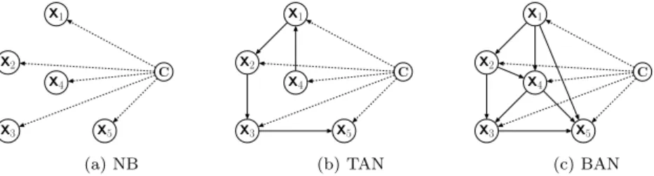
Na¨ıve Bayes (NB) is a well-known Bayesian classifier which is very computa-tionally efficient and has in general good predictive performance. NB is based on the assumption that features are independent from each other, given the class variable. An example network topology is shown in Figure 1(a), where the edges indicate that each feature depends only on the class (their only par-ent node). To classify a testing instance, NB computes the probability of each
class labelc given all the feature values (x1,x2,...,xm) of the instance using
Equation (1) – where the symbol∝means “proportional to” – and assigns the
instance to the class label with the greatest probability.
P
(
c
|
x
1, x
2, ..., x
m)
∝
P
(
c
)
mQ
i=1P
(
x
i|
c
)
(1)In Equation (1),mis the number of features, and the probability of a class
label c given all feature values of an instance is estimated by calculating the
product of the prior probability ofctimes the probability of each feature value
xigiven c, using the above mentioned independence assumption.
2.2 The Tree Augmented Na¨ıve Bayes (TAN) Classifier
TAN is a type of semi-Na¨ıve Bayes classifier that relaxes Na¨ıve Bayes’ feature independence assumption, by allowing each feature to depend on at most one other feature – in addition to depending on the class, which is a parent node of all features. An example network topology is shown in Figure 1(b), where
all nodes except X4 have one non-class variable parent node. This increases
the ability to represent feature dependencies (which may lead to improved predictive accuracy) and still leads to reasonably efficient algorithms. TAN algorithms are not as efficient (fast) as NB, but TAN algorithms are in general much more efficient and scalable than other Bayesian classification algorithms that allow a feature to depend on several features. Among the several types of TAN algorithms, e.g., in (Friedman et al 1997; Keogh and Pazzani 1999; Jiang
et al 2005; Zhang and Ling 2001), in this work we focus on one of the most computationally efficient ones, which is based on the principle of maximizing the conditional mutual information (CMI) for each pair of features given the class attribute (Friedman et al 1997). Then, the Maximum Weight Spanning Tree (MST) is built, where the weight of an edge is given by its CMI. Finally, one vertex of the MST is randomly selected as the root, and the edge directions are propagated accordingly.
2.3 The Bayesian Network Augmented Na¨ıve Bayes (BAN) Classifier
Compared with Na¨ıve Bayes and TAN classifiers, a Bayesian Network Aug-mented Na¨ıve Bayes (BAN) classifier is a type of more sophisticated semi-Na¨ıve Bayes classifier that allows each feature to have more than one parents. An
example network topology is shown in Figure 1(c), where node X4 has two
parent nodes, i.e., X1and X2. The conventional algorithm to construct a BAN
is analogous to the one for learning the TAN classifier (Friedman et al 1997). In this work, instead of learning the feature dependencies by conventional methods, we use the GO–hierarchy–aware BAN (GO–BAN) classifier proposed in (Wan and Freitas 2013, 2015), hereafter denoted simply BAN, where the net-work edges representing feature dependencies are simply the pre-defined edges in the feature hierarchy. More precisely, this BAN classifier uses the edges of the Gene Ontology (GO)’s DAG (Directed Acyclic Graph) (The Gene Ontol-ogy Consortium 2000) – see Section 2.6 – as the topolOntol-ogy of the BAN network. This has the advantages of saving computational time and exploiting the back-ground knowledge associated with the Gene Ontology, which incorporates the expertise of a large number of biologists.
X1 X2 X3 X5 X4 C (a) NB X1 X2 X3 X5 X4 C (b) TAN X1 X2 X3 X5 X4 C (c) BAN
Fig. 1: Topology of different Bayesian network classifiers
2.4 TheK-Nearest Neighbors Classifier (KNN)
K-Nearest Neighbors is a “lazy learning”-based classifier (see Section 2.5). It
classifies an individual testing instance by assigning to it the class label of
the majority of itsk nearest training instances (Hastie et al 2001; Aha 1997;
Cover and Hart 1967). In this work, the3 nearest training instances were used
for classification. We adopt the Jaccard similarity coefficient (Jain and Dubes 1988; Jain and Zongker 1997) as the distance measure, due to the fact that in the datasets used in this work the features take binary values. As shown in
Equation (2), the Jaccard similarity coefficient measures the ratio of the size of the intersection over the size of the union of two feature sets,
Jaccard(i, k)= m11
m11+m10+m01 (2)
wherem11denotes the number of features with value “1” in both theith
(test-ing) andkth(nearest training) instances;m10 denotes the number of features
with value “1” in theith instance and value “0” in thekthinstance; m01
de-notes the number of features with value “0” in theithinstance and value “1”
in thekthinstance. A greater value of the Jaccard coefficient means a smaller
distance (higher similarity) between the two instances.
2.5 Lazy Learning
A “lazy” learning method performs the learning process in the testing phase, building a specific classification model for each new testing instance to be classified (Aha 1997; Pereira et al 2011). This is in contrast to the usual “eager” learning approach, where a classification model is learnt from the training instances before any testing instance is observed. In the context of feature selection, lazy learning selects a specific set of features for each individual testing instance, whilst eager learning selects a single set of features for all testing instances. Some hierarchical feature selection methods evaluated in this work are lazy methods, because they exploit hierarchical information which is specific to each instance, in order to select the best set of features for each instance – as described later. Hence, we use lazy versions of NB, TAN and BAN, as well as KNN (which is naturally lazy), in our experiments.
2.6 The Gene Ontology and Hierarchical Feature Redundancy
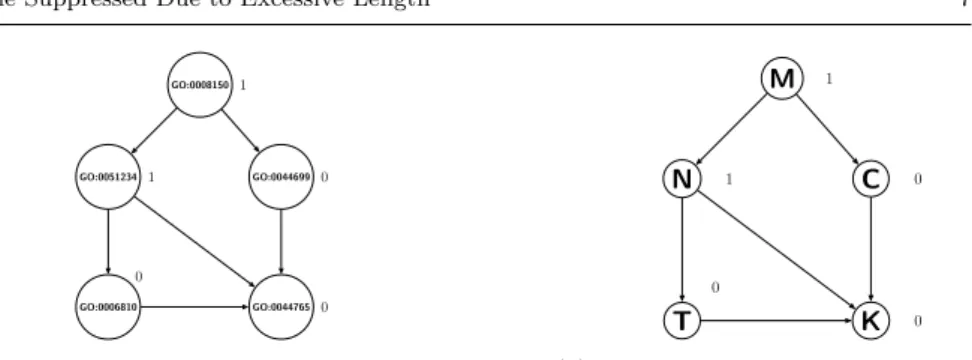
The Gene Ontology (GO) uses unified and structured controlled vocabularies to describe gene functions (The Gene Ontology Consortium 2000). There are three types of GO terms: biological process, molecular function and cellular component. Most GO terms are hierarchically structured by an “is-a” rela-tionship, where each GO term is a specialization of its ancestor (more generic) terms. Therefore, there are three DAGs representing the three types of GO terms. For example, as shown in Figure 2(a), GO:0008150 (biological process) is the root of the DAG for biological process terms, and it is also the parent of GO:0051234 (establishment of localization), which is in turn the parent of GO:0006810 (transport).
Consider a hierarchy of features, where each feature represents a GO term which is a node in a GO DAG. Each feature takes a binary value, “1” or “0”, indicating whether or not an instance (a gene) is annotated with the corre-sponding GO term. The “is-a” hierarchy of the GO is associated with two hierarchical constraints. First, if a feature takes the value “1” for a given in-stance, this implies its ancestors in the DAG also take the value “1” for that instance. For example, in Figure 2(a), if the term GO:0051234 has value “1”
GO:0008150 GO:0051234 GO:0006810 GO:0044699 GO:0044765 1 1 0 0 0
(a) A small part of the Gene Ontology’s topology
M N T C K 1 1 0 0 0
(b) Example of hierarchical redundancy
Fig. 2: Example of hierarchically structured features
for a given gene, then the value of term GO:0008150 should be “1” as well. Conversely, if the feature takes the value “0” for a given instance, this implies that its descendants in the DAG also take the value “0” for that instance. For example, if the term GO:0006810 has value “0”, then term GO:0044765 should also have value “0”.
Hierarchical feature redundancy is defined in this work as the case where there are two or more nodes which have the same value (“1” or “0”) in an in-dividual instance and are located in the same path from a root to a leaf node in the DAG. For instance, in Figure 2(b), where the number “1” or “0” beside a node is the value of that feature in a given instance, nodes N and M are redundant, since both have value “1” and are located in the same path, i.e., M–N–T–K or M–N–K. Analogously, nodes T and K are redundant, since both have value “0” and are in the same path M–N–T–K. Nodes C and K are also redundant, since both have value “0” and are in the path M–C–K. Removing this type of hierarchical feature redundancy is the core task performed by the hierarchical feature selection methods used in this work.
The problem of hierarchical feature selection as addressed in this paper is
defined as follows:Given a set of m features organized into a feature hierarchy
(a tree or a DAG) encoding “is-a” relationships, the goal is to select a subset of s features (1 ≤s≤m) which has reduced hierarchical redundancy, by com-parison with the full set of m features, while still preserving features which are useful for discriminating among the classes.
3 Hierarchical Feature Selection Methods – Select Hierarchical Information-Preserving (HIP) Features and Select Most Relevant (MR) Features
In our previous works (Wan and Freitas 2013; Wan et al 2015; Wan and Freitas 2015; Wan 2015), we proposed three lazy learning-based hierarchical feature selection methods to cope with the hierarchical feature redundancy issue discussed in Section 2.6. These methods are called Select Hierarchical Information-Preserving (HIP) features, Select Most Relevant (MR) features, and the hybrid HIP–MR method. In general, both HIP and MR select a set of
features without hierarchical redundancy, whereas HIP–MR usually generates a set of features where the redundancy issue is only alleviated, but not elimi-nated (Wan et al 2015). Hence, both HIP and MR select much fewer features, and they obtained substantially greater predictive accuracy than the hybrid HIP–MR in the experiments reported in (Wan et al 2015). Hence, we use only HIP and MR in this work.
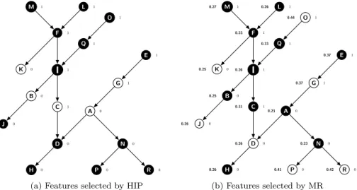
HIP and MR perform “lazy” feature selection, i.e., they select a specific set of features for each testing instance, based on the feature values observed in that instance. The HIP method selects only features whose values are not implied by the value of any other feature in the current testing instance, due to the hierarchical constraints (see Section 2.6). For instance, in Figure 3(a), the value of node (feature) C is not implied by any other feature’s value, but its value “1” implies that the values of its ancestors I, F, M, L, Q and O are also “1”; the value of node A is also not implied by any other feature’s value, but its value “0” implies that the values of nodes D, H, N, P and R are also “0”. HIP will select nodes K, B, C, A and G for the example DAG of Figure 3(a), since this feature subset preserves all the hierarchical information – i.e., for any given instance, the values of the features in this subset imply the values of all the other features.
F I C D K L B J H A G E M Q O N P R 1 1 0 1 0 0 1 0 0 0 1 1 1 1 1 0 0 0
(a) Features selected by HIP
F I C D K L B J H A G E M Q O N P R 0.23 0.26 0.31 0.26 0.25 0.26 0.25 0.26 0.26 0.23 0.37 0.37 0.27 0.23 0.41 0.42 0.33 0.44 1 1 0 1 0 0 1 0 0 0 1 1 1 1 1 0 0 0 (b) Features selected by MR
Fig. 3: Example of hierarchical feature selection by HIP and MR
The MR method selects the feature with maximal relevance value in the set of features whose values equal to “1” or “0” in each path of the feature DAG. If there exist more than one features having the maximal relevance value, only the deepest (most specific) one (if the feature value is “1”) or the shallowest (most generic) one (if the feature value is “0”) in that path will be selected. There are many different functions that can be used to evaluate the quality of a feature, such as information gain, chi-squared, etc. In the MR algorithm,
as proposed in (Wan and Freitas 2013; Wan et al 2015), Equation (3) is used to
measure the relevance (R) (predictive power) of a binary feature X, which can
take value x1 or x2. In this equation,n denotes the number of classes and ci
denotes thei-th class label. Equation (3) measures the relevance of a feature as
a function of the difference in the conditional probabilities of each class given different values (“1” or “0”) of the feature. This equation, which was adapted from a similar equation for measuring feature relevance proposed in (Stanfill and Waltz 1986), was chosen because it is simple to interpret in probabilistic terms as a direct measure of a feature’s relevance for class discrimination, and so it is naturally compatible with the use of Bayesian classification network algorithms in our experiments. Future work could experiment with different feature evaluation functions.
R(X) =
n
X
i=1
[P(ci|x1)−P(ci|x2)]2 (3)
In the example DAG in Figure 3(b), where the numbers on the left side of nodes denote the corresponding relevance values and the numbers on the right side of nodes denote the binary feature values, the MR method selects 7 nodes, namely K, J, D, P, R, G and O. In detail, MR selects node O rather than node Q, since the former has higher relevance value and both nodes have the value “1” in the same path; and it selects node G rather than node E, since the former is deeper than the latter and both nodes have value “1” in the same path. Analogously, MR selects node J rather than node B, since the former has higher relevance value and both nodes have the value “0” in the same path; and it selects node D rather than node H, since the former is shallower and both nodes have value “0” in the same path. Note that, in this case, the features selected by MR will lead to some hierarchical information loss. For example, the value “1” of selected node O does not imply that the value of non-selected node Q is also “1”, and the Q’s value is not implied by the value of any selected node (so the information that Q has value “1” was lost). Similarly, the value “0” of selected node J does not imply that non-selected node B has value “0”, and B’s value is not implied by the value of any selected node.
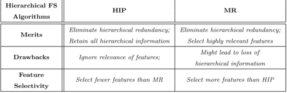
Table 1: Summary of characteristics of the HIP and MR methods
Hierarchical FS
HIP MR
Algorithms
Merits Eliminate hierarchical redundancy; Eliminate hierarchical redundancy;
Retain all hierarchical information Select highly relevant features
Drawbacks Ignore relevance of features; Might lead to loss of hierarchical information
Feature
Select fewer features than MR Select more features than HIP
As summarized in Table 1, both HIP and MR have the merit of elimi-nating hierarchical feature redundancy. However, they differ in other aspects, with their own merits and drawbacks, i.e., HIP selects features retaining all hierarchical information whilst ignoring the relevance of features with the class attribute; whereas MR selects features having higher relevance to the class at-tribute, but the selected features might not retain the complete hierarchical information (i.e., leading to loss of hierarchical information).
The program codes of HIP and MR (in Java) are freely available from
https://github.com/andywan0125/AIRE-Journal.
4 Experimental Methodology and Computational Results
4.1 Dataset Creation
We constructed 28 datasets with data about the effect of genes on an organ-ism’s longevity, by integrating data from the Human Ageing Genomic
Re-sources (HAGR) GenAge database (Build 17) (de Magalh˜aes et al 2009) and
the Gene Ontology (GO) database (version: 2014-06-13) (The Gene Ontol-ogy Consortium 2000). HAGR provides longevity-related gene data for four
model organisms, i.e.,C. elegans (worm),D. melanogaster (fly),M. musculus
(mouse) and S. cerevisiae (yeast). For details of the dataset creation
proce-dure, see (Wan and Freitas 2013; Wan et al 2015). However, in (Wan and Freitas 2013; Wan et al 2015) we created datasets using only Biological Pro-cess GO terms; whilst in this current work we created datasets with all three types of GO terms, each type associated with a hierarchy (see Section 2.6) in the form of a DAG: Biological Process (BP), Molecular Function (MF) and Cellular Component (CC) GO terms. Note that the different types of GO terms are contained in DAGs whose sets of nodes do not intersect with each other. This means that the hierarchical feature selection methods conduct the feature selection process based on each individual DAG separately.
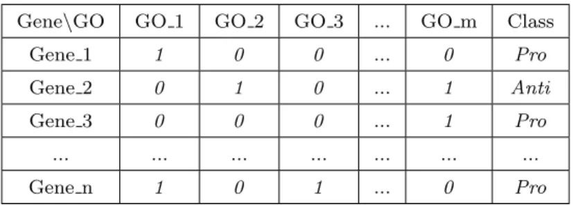
Gene\GO GO 1 GO 2 GO 3 ... GO m Class Gene 1 1 0 0 ... 0 Pro Gene 2 0 1 0 ... 1 Anti Gene 3 0 0 0 ... 1 Pro ... ... ... ... ... ... ... Gene n 1 0 1 ... 0 Pro
In the created datasets, the instances represent aging-related genes, the fea-tures represent hierarchical GO terms, and the class variable indicates whether the gene contributes to increasing or decreasing the longevity of an organism. For each model organism, we created 7 datasets, with all possible subsets of the three GO term types, i.e., one dataset for each GO term type (BP, MF, CC), one dataset for each pair of GO term types (BP and MF, BP and CC, MF and CC), and one dataset with all 3 GO term types (BP, MF and CC). The struc-ture of each created dataset is shown in Figure 4, where the feastruc-ture value “1” or “0” indicates whether or not (respectively) a GO term is annotated for each gene. In the class variable, the values “Pro” and “Anti” mean “pro-longevity” and “anti-longevity”. Pro-longevity genes are those whose decreased expression (due to knock–out, mutations or RNA interference) reduces lifespan and/or whose overexpression extends lifespan. Anti-longevity genes are those whose decreased expression extends lifespan and/or whose overexpression decreases lifespan (Tacutu et al 2013).
Note that GO terms with only one associated gene would be useless for building a classification model because they are extremely specific to an indi-vidual gene, and a model that includes these GO terms would be over-fitting the data. However, GO terms associated with only a few genes might be valu-able for discovering biological knowledge, since they might represent specific biological information. In our previous work (Wan et al 2015), we did experi-ments with different values of a threshold defining the minimum frequency of occurrence of a GO term which is required in order to include that term (as a feature) in a dataset, in order to perform effective classification. Based on that work, the threshold value of at least 3 occurrences is used here, which retains more biological information than higher thresholds while still leading to high predictive accuracy. In addition, the root GO terms – i.e., GO:0008150, GO:0003674 and GO:0005575, respectively for the DAG of biological process, molecular function and cellular component terms – are not included in the corresponding datasets, since the root GO terms have no predictive power (all genes are trivially annotated with each root GO term).
The main characteristics of the created datasets are shown in Table 2, which reports the number of features and edges in the GO DAG, the total number of instances, the number (and percentage) of instances in each class, and the degree of class imbalance. The degree of class imbalance is calculated
by Equation (4), where the degree (D) equals to the complement of the ratio
of the number of instances belonging to the minority class (No(M inor)) over
the number of instances belonging to the majority class (No(M ajor)).
D= 1−N
o(M inor)
No(M ajor) (4)
All datasets used in our experiments are freely available from https://
Table 2: Main characteristics of the created datasets Caenorhabditis elegans (worm)
Feature (GO term) type BP MF CC BP+MF BP+CC MF+CC BP+MF+CC
Noof Features 830 218 143 1048 973 361 1191 Noof Edges 1437 259 217 1696 1654 476 1913 Noof Instances 528 279 254 553 557 432 572 No(%) of Pro- 209 121 98 213 213 170 215 Longevity Instances 39.6% 43.4% 38.6% 38.5% 38.2% 39.4% 37.6% No(%) of Anti- 319 158 156 340 344 262 357 Longevity Instances 60.4% 56.6% 61.4% 61.5% 61.8% 60.6% 62.4%
Degree of Class Imbalance 0.345 0.234 0.372 0.374 0.381 0.351 0.398
Drosophila melanogaster (fly)
Feature (GO term) type BP MF CC BP+MF BP+CC MF+CC BP+MF+CC
Noof Features 698 130 75 828 773 205 903 Noof Edges 1190 151 101 1341 1291 252 1442 Noof Instances 127 102 90 130 128 123 130 No(%) of Pro- 91 68 62 92 91 85 92 Longevity Instances 71.7% 66.7% 68.9% 70.8% 71.1% 69.1% 70.8% No(%) of Anti- 36 34 28 38 37 38 38 Longevity Instances 28.3% 33.3% 31.1% 29.2% 28.9% 30.9% 29.2%
Degree of Class Imbalance 0.604 0.500 0.548 0.587 0.593 0.553 0.587
Mus musculus (mouse)
Feature (GO term) type BP MF CC BP+MF BP+CC MF+CC BP+MF+CC
Noof Features 1039 182 117 1221 1156 299 1338 Noof Edges 1836 205 160 2041 1996 365 2201 Noof Instances 102 98 100 102 102 102 102 No(%) of Pro- 68 65 66 68 68 68 68 Longevity Instances 66.7% 66.3% 66.0% 66.7% 66.7% 66.7% 66.7% No(%) of Anti- 34 33 34 34 34 34 34 Longevity Instances 33.3% 33.7% 34.0% 33.3% 33.3% 33.3% 33.3%
Degree of Class Imbalance 0.500 0.492 0.485 0.500 0.500 0.500 0.500
Saccharomyces cerevisiae (yeast)
Feature (GO term) type BP MF CC BP+MF BP+CC MF+CC BP+MF+CC
Noof Features 679 175 107 854 786 282 961 Noof Edges 1223 209 168 1432 1391 377 1600 Noof Instances 215 157 147 222 234 226 238 No(%) of Pro- 30 26 24 30 30 29 30 Longevity Instances 14.0% 16.6% 16.3% 13.5% 12.8% 12.8% 12.6% No(%) of Anti- 185 131 123 192 204 197 208 Longevity Instances 86.0% 83.4% 83.7% 86.5% 87.2% 87.2% 87.4%
4.2 Experimental Methodology and Predictive Accuracy Measure
We evaluate the two previously described hierarchical feature selection meth-ods (HIP and MR) by comparing them with two other hierarchical feature selection methods (SHSEL and GTD) and one “flat” feature selection method (CFS). In essence, the SHSEL method selects the features having more rel-evance and less redundancy with respect to other features in the same path
in the feature hierarchy. It consists of two stages (we used thepruneSHSEL
version, see (Ristoski and Paulheim 2014)). Firstly, it starts from each leaf node of the feature hierarchy, removing the features having a relevance value similar to their parent nodes’ relevance values – in this work, we adopt 0.99 as the threshold value for considering two features as similar, as suggested by (Ristoski and Paulheim 2014). Then, in the second stage, SHSEL continues to remove the features whose relevance values are less than the average relevance value for all remaining features in the corresponding path.
The GTD method is based on the greedy top-down search strategy (Lu et al 2013). It sorts features in each individual path according to their rele-vance values and selects the feature having the highest relerele-vance value in each path, and then removes all other features in the path. In this work, the measure used for evaluating a feature’s relevance value is the well-known Information Gain for both the SHSEL and GTD methods.
CFS is a well-known feature selection method that tries to select a feature subset where each feature has a high correlation with the class variable and the features have a low correlation with each other (to avoid selecting redun-dant features). Hence, CFS is an interesting baseline method because it tries to remove redundant features in a “flat” sense, without exploiting the notion of hierarchically redundant features that is at the core of HIP and MR.
Note that SHSEL, GTD and CFS follow the conventional eager learning ap-proach, i.e., they select the same feature subset to classify all testing instances. By contrast, HIP and MR follow the lazy learning approach (see Section 2.5), performing feature selection separately for each testing instance. This gives HIP and MR the flexibility to cope with a finer-grained concept of hierarchi-cal redundancy, which depends on each instance’s specific feature values, as discussed in Section 2.6.
We perform four sets of experiments, using NB, TAN, BAN and KNN as classifiers. The well-known 10-fold cross validation procedure was adopted to evaluate the predictive performance of these classifiers with different feature selection methods. The Geometric Mean (GMean) of the Sensitivity (Sen.) and Specificity (Spe.) is used to measure predictive accuracy, since the distri-butions of classes in the datasets are imbalanced. As shown in Equation (5),
GMean is defined as the square root of the product of Sen. and Spe.; Sen.
denotes the percentage of positive (“pro-longevity”) instances that are
cor-rectly classified as positive, whereas Spe. denotes the percentage of negative
(“anti-longevity”) instances that are correctly classified as negative.
4.3 Experimental Results
4.3.1 Feature selection results separately for each Bayesian classifier and the K-Nearest Neighbors classifier
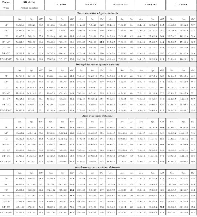
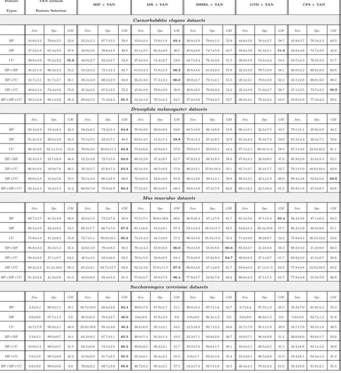
Tables 3, 4, 5 and 6 report the feature selection results separately for each type of classifier, namely Na¨ıve Bayes, TAN, BAN and KNN, respectively. These tables have the same structure, reporting the results for 5 different fea-ture selection methods in a pre-processing phase, namely 4 hierarchical feafea-ture selection methods (HIP, MR, SHSEL, GTD) and the “flat” feature selection method CFS; and also reporting results for not using any feature selection method – so, 6 approaches are compared in total. Each table contains the results for 28 datasets – 7 combinations of feature (GO term) types for each of 4 model organisms. In each table, the best GMean value for each dataset is shown in boldface. For each of the 28 datasets in each table, we compute a ranking of the feature selection methods, where ranks 1 and 6 represent the best and worst GMean values, respectively, in that dataset.
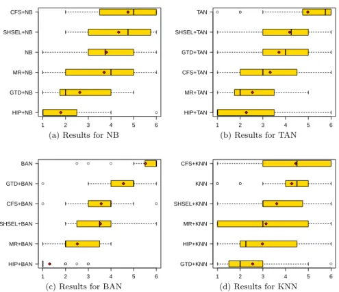
The distributions of rank values (across the 28 datasets) for different fea-ture selection methods with different classifiers are shown in the boxplots in Figures 5(a)-5(d), which summarize the results of Tables 3–6 for NB, TAN, BAN and KNN, respectively. Each boxplot consists of a box whose left and right boundaries denote the lower and upper quartile (respectively) of a dis-tribution of rank values. The vertical line between these quartiles denotes the median rank value, the red diamond denotes the average (mean) rank value, and the horizontal lines extending from the left and the right boundaries of the box end with vertical lines that denote the smallest and highest (respec-tively) non-outlier rank values. Outliers are shown as separate points in the plot. The difference between the upper and lower quartiles is the inter-quartile range, and 50% of the rank values fall into this range. Note that in each of Figures 5(a)-5(d) the boxplots of different feature selection methods are sorted across the vertical axis according to their average rank – i.e., the boxplot of the method with the lowest (best) average rank is at the bottom of the figure. Table 3 reports the predictive accuracies obtained by Na¨ıve Bayes. As shown in Figure 5(a), HIP obtained the lowest (best) median rank (1.0) and average rank (1.8), as well as the lowest lower and upper quartiles. The in-terquartile range of HIP’s ranks is the narrowest among all methods, indicating the small variability of its rank values across datasets. GTD+NB obtained the second best median rank (2.0) and average rank (2.6). The other methods obtained substantially worse results, with the following average and median ranks, respectively: 3.7 and 4.0 for MR, 3.8 and 3.8 for NB without feature selection, 4.3 and 4.8 for SHSEL, 4.8 and 5.0 for CFS.
Table 4 reports the predictive accuracies obtained by TAN. As shown in Figure 5(b), HIP obtained again the best median rank (1.0) and average rank (2.3); followed by MR, with median rank 2.0 and average rank 2.5. The other methods obtained substantially worse results, with the following average and median ranks, respectively: 3.3 and 3.0 for CFS, 3.7 and 4.0 for GTD, 4.2 and
● HIP+NB GTD+NB MR+NB NB SHSEL+NB CFS+NB 1 2 3 4 5 6
(a) Results for NB
● ● ● HIP+TAN MR+TAN CFS+TAN GTD+TAN SHSEL+TAN TAN 1 2 3 4 5 6
(b) Results for TAN
● ● ● ●● ● ● ● ● ● ● ● HIP+BAN MR+BAN SHSEL+BAN CFS+BAN GTD+BAN BAN 1 2 3 4 5 6
(c) Results for BAN
● ● ● ● ● GTD+KNN HIP+KNN MR+KNN SHSEL+KNN KNN CFS+KNN 1 2 3 4 5 6 (d) Results for KNN
Fig. 5: Boxplots showing the distributions of ranks obtained by different feature selection methods with each of 4 classifiers
4.3 for SHSEL, 5.0 and 5.8 for TAN without feature selection.
Table 5 reports the predictive accuracies obtained by BAN. As shown in Figure 5(c), HIP obtained again the best median rank (1.0) and average rank (1.3); and it has an extremely small inter-quartile range, so even the upper quartile of its ranks is substantially lower (better) than the lower quartile of all other methods. Hence, HIP clearly outperformed all other methods, whose average and median ranks are, respectively: 2.5 and 2.0 for MR, 3.5 and 3.5 for SHSEL, 3.6 and 4.0 for CFS, 4.6 and 5.0 for GTD, 5.5 and 6.0 for BAN without feature selection.
Table 6 reports the predictive accuracies obtained by KNN. As shown in Figure 5(d), GTD obtained the best median rank (2.0) and average rank (2.6); followed by HIP, with median rank 2.3 and average rank 3.0. The other meth-ods obtained the following average and median ranks, respectively: 3.1 and 3.0 for MR, 3.6 and 3.0 for SHSEL, 4.3 and 4.5 for KNN without feature selection, 4.5 and 4.5 for CFS.
Table 3: Predictive accuracy (%) for Na¨ıve Bayes with hierarchical feature selection methods HIP, MR, SHSEL, GTD and “flat” feature selection method CFS
Feature NB without
HIP + NB MR + NB SHSEL + NB GTD + NB CFS + NB
Types Feature Selection
Caenorhabditis elegans datasets
Sen. Spe. GM Sen. Spe. GM Sen. Spe. GM Sen. Spe. GM Sen. Spe. GM Sen. Spe. GM BP 50.2±3.6 69.0±2.6 58.9 54.1±3.4 75.5±2.8 63.9 51.2±3.5 75.5±2.6 62.2 50.2±4.1 74.3±2.5 61.1 63.2±4.1 65.8±2.9 64.5 41.1±3.3 83.7±2.6 58.7 MF 57.9±4.1 46.2±5.5 51.7 45.5±4.7 51.9±5.1 48.6 38.8±2.9 63.3±3.8 49.6 36.4±5.7 70.9±5.6 50.8 52.9±3.1 55.1±5.4 54.0 58.7±6.8 46.8±5.5 52.4 CC 43.9±5.7 70.5±3.4 55.6 58.2±4.9 60.9±4.0 59.5 42.9±4.0 71.2±3.0 55.3 34.7±3.4 76.3±3.7 51.5 46.9±5.0 67.9±3.6 56.4 35.7±4.3 74.4±3.9 51.5 BP+MF 54.0±1.8 70.3±3.0 61.6 53.5±3.6 76.2±1.9 63.8 62.9±3.5 73.2±1.8 67.9 51.2±3.5 75.6±1.8 62.2 61.5±3.2 67.4±2.7 64.4 50.2±3.5 77.1±2.4 62.2 BP+CC 52.6±3.9 68.3±2.6 59.9 57.7±3.7 73.0±2.6 64.9 55.4±2.8 73.8±2.2 63.9 49.3±2.6 73.5±2.4 60.2 57.3±3.7 70.1±2.1 63.4 44.6±3.7 77.0±2.2 58.6 MF+CC 51.2±2.8 64.1±4.3 57.3 54.7±3.3 66.0±4.1 60.1 47.6±3.6 68.3±4.2 57.0 42.4±3.4 73.7±3.5 55.9 52.4±2.7 66.4±4.7 59.0 47.1±3.9 72.1±3.8 58.3 BP+MF+CC 52.1±4.4 70.0±2.3 60.4 55.3±3.6 71.7±2.7 63.0 55.8±3.6 70.6±2.4 62.8 49.8±4.4 70.9±2.3 59.4 54.4±3.5 69.2±2.3 61.4 51.6±4.4 74.8±2.1 62.1
Drosophila melanogaster datasets
Sen. Spe. GM Sen. Spe. GM Sen. Spe. GM Sen. Spe. GM Sen. Spe. GM Sen. Spe. GM BP 74.7±3.5 36.1±9.5 51.9 73.6±4.1 44.4±9.0 57.2 79.1±4.1 38.9±11.0 55.5 74.7±5.2 41.7±9.6 55.8 75.8±3.8 41.7±7.9 56.2 76.9±4.7 27.8±7.4 46.2 MF 82.4±4.6 35.3±8.6 53.9 69.1±6.1 52.9±7.3 60.5 80.9±4.2 44.1±7.6 59.7 77.9±5.5 41.2±8.3 56.7 83.8±5.4 35.3±6.4 54.4 86.8±4.0 35.3±7.2 55.4 CC 87.1±4.1 50.0±10.2 66.0 80.6±6.5 46.4±11.4 61.2 83.9±5.6 53.6±8.7 67.1 85.5±3.9 25.0±5.1 46.2 88.7±4.3 53.6±11.2 69.0 87.1±3.3 39.3±10.0 58.5 BP+MF 77.2±3.9 50.0±10.2 62.1 72.8±5.6 57.9±9.3 64.9 79.3±4.3 44.7±8.2 59.5 81.5±3.8 44.7±9.2 60.4 77.2±3.6 42.1±6.5 57.0 85.9±3.7 31.6±7.5 52.1 BP+CC 76.9±5.1 48.6±9.8 61.1 73.6±4.9 64.9±8.3 69.1 80.2±4.3 56.8±11.2 67.5 79.1±3.4 45.9±8.7 60.3 76.9±4.6 48.6±9.8 61.1 82.4±3.7 43.2±10.9 59.7 MF+CC 89.4±3.2 57.9±5.3 71.9 82.4±6.1 63.2±6.7 72.2 83.5±4.4 57.9±7.5 69.5 88.2±3.5 50.0±5.3 66.4 91.8±3.5 57.9±5.3 72.9 91.8±3.4 42.1±8.4 62.2 BP+MF+CC 81.5±5.3 55.3±8.2 67.1 76.1±4.9 68.4±5.3 72.1 77.2±4.5 63.2±7.7 69.9 84.8±3.4 57.9±8.4 70.1 78.3±4.7 57.9±6.5 67.3 90.2±3.1 47.4±8.7 65.4
Mus musculus datasets
Sen. Spe. GM Sen. Spe. GM Sen. Spe. GM Sen. Spe. GM Sen. Spe. GM Sen. Spe. GM BP 82.4±4.7 44.1±5.9 60.3 72.1±4.8 70.6±5.1 71.3 80.9±5.2 50.0±7.9 63.6 85.3±4.3 47.1±7.0 63.4 83.8±5.0 44.1±5.9 60.8 83.8±4.0 38.2±5.6 56.6 MF 69.2±7.4 48.5±11.2 57.9 78.5±4.4 45.5±12.2 59.8 83.1±4.1 39.4±10.7 57.2 83.1±4.5 30.3±11.8 50.2 81.5±5.5 42.4±11.1 58.8 80.0±5.2 36.4±10.5 54.0 CC 75.8±2.3 52.9±10.0 63.3 80.3±3.0 47.1±11.2 61.5 81.8±3.6 41.2±11.9 58.1 77.3±3.3 50.0±10.1 62.2 75.8±2.3 52.9±10.0 63.3 71.2±3.0 35.3±11.2 50.1 BP+MF 83.8±3.4 44.1±7.0 60.8 70.6±4.8 70.6±8.1 70.6 82.4±4.2 50.0±10.2 64.2 86.8±4.0 47.1±7.7 63.9 83.8±4.5 44.1±7.0 60.8 88.2±4.2 41.2±8.0 60.3 BP+CC 79.4±6.1 50.0±8.4 63.0 66.2±5.0 73.5±9.3 69.8 73.5±5.1 52.9±9.6 62.4 82.4±5.1 55.9±10.5 67.9 77.9±5.7 52.9±9.6 64.2 83.8±5.0 50.0±11.3 64.7 MF+CC 75.0±5.0 64.7±12.5 69.7 79.4±4.2 58.8±11.8 68.3 83.8±5.0 55.9±13.3 68.4 86.8±4.6 50.0±11.7 65.9 76.5±5.1 58.8±13.0 67.1 77.9±4.8 47.1±10.9 60.6 BP+MF+CC 82.4±4.2 47.1±9.3 62.3 73.5±5.1 73.5±9.8 73.5 85.3±4.3 50.0±6.9 65.3 86.8±4.5 55.9±7.0 69.7 83.8±4.0 47.1±9.3 62.8 83.8±3.3 52.9±6.8 66.6
Saccharomyces cerevisiae datasets
Sen. Spe. GM Sen. Spe. GM Sen. Spe. GM Sen. Spe. GM Sen. Spe. GM Sen. Spe. GM BP 40.0±8.3 84.9±3.5 58.3 63.3±6.0 78.4±3.1 70.4 33.3±8.6 85.9±2.9 53.5 20.0±5.4 93.0±2.1 43.1 43.4±7.1 86.5±2.9 61.3 20.0±5.4 91.4±2.6 42.8 MF 11.5±6.1 81.7±4.8 30.7 5.0±5.0 83.2±3.4 20.4 0.0±0.0 93.9±2.4 0.0 0.0±0.0 96.9±1.3 0.0 11.5±6.1 86.3±2.9 31.5 5.0±5.0 92.4±1.8 21.5 CC 25.0±7.1 86.2±3.0 46.4 29.2±10.2 82.9±4.2 49.2 20.8±6.9 91.9±2.7 43.7 20.8±7.5 89.4±2.6 43.1 25.0±7.1 87.0±3.2 46.6 20.8±7.5 94.3±1.7 44.3 BP+MF 33.3±11.1 85.4±1.7 53.3 76.7±7.1 74.0±3.3 75.3 23.3±5.1 89.1±2.5 45.6 30.0±9.2 92.2±2.1 52.6 46.7±10.2 88.0±1.6 64.1 33.3±9.9 90.6±1.5 54.9 BP+CC 53.3±8.9 85.8±3.0 67.6 70.0±7.8 79.4±3.2 74.6 40.0±8.3 84.8±2.7 58.2 30.0±6.0 92.6±2.0 52.7 53.3±5.4 89.2±2.6 69.0 40.0±8.3 91.2±1.8 60.4 MF+CC 34.5±10.5 87.3±2.1 54.9 31.0±8.0 82.2±3.5 50.5 17.2±6.3 89.8±2.3 39.3 13.8±6.3 91.4±1.7 35.5 34.5±9.2 89.8±1.3 55.7 13.8±6.3 91.9±1.9 35.6 BP+MF+CC 36.7±9.2 85.6±2.7 56.0 70.0±10.5 75.0±2.6 72.5 30.0±9.2 86.5±2.6 50.9 49.8±4.4 70.9±2.3 59.4 54.4±3.5 69.2±2.3 61.4 36.7±10.5 92.8±1.9 58.4
Table 4: Predictive accuracy (%) for TAN with hierarchical feature selection methods HIP, MR, SHSEL, GTD and “flat” feature selection method CFS Feature TAN without
HIP + TAN MR + TAN SHSEL + TAN GTD + TAN CFS + TAN
Types Feature Selection
Caenorhabditis elegans datasets
Sen. Spe. GM Sen. Spe. GM Sen. Spe. GM Sen. Spe. GM Sen. Spe. GM Sen. Spe. GM BP 34.0±3.2 79.6±2.3 52.0 52.2±2.3 67.7±3.5 59.4 55.0±2.4 73.0±1.8 63.4 36.8±3.9 79.0±1.5 53.9 44.0±3.6 78.4±2.7 58.7 45.9±3.7 79.3±2.2 60.3 MF 37.2±5.8 61.4±5.0 47.8 43.0±5.6 50.6±4.5 46.6 33.1±3.5 65.2±4.0 46.5 25.6±4.6 74.7±5.9 43.7 43.8±3.8 61.4±5.1 51.9 24.8±4.8 74.7±4.0 43.0 CC 39.8±3.0 78.2±2.2 55.8 44.9±2.7 62.2±4.7 52.8 37.8±3.4 74.4±2.7 53.0 34.7±3.4 76.3±3.6 51.5 39.8±3.0 74.4±2.4 54.4 34.7±4.3 76.9±3.2 51.7 BP+MF 35.2±1.9 80.3±2.2 53.2 54.5±3.2 72.1±2.4 62.7 61.0±4.3 71.8±2.3 66.2 40.8±3.6 81.8±2.0 57.8 42.3±3.9 79.7±0.9 58.1 46.0±3.2 80.6±2.0 60.9 BP+CC 42.7±3.1 81.7±2.7 59.1 59.2±3.9 69.2±2.9 64.0 56.3±3.0 77.3±2.2 66.0 39.0±2.7 79.1±2.1 55.5 48.4±3.1 79.9±2.8 62.2 45.1±2.8 80.8±2.0 60.4 MF+CC 40.6±3.4 74.4±3.6 55.0 45.3±2.2 67.2±3.5 55.2 45.9±3.8 70.6±3.0 56.9 38.8±2.5 76.0±3.2 54.3 45.3±3.8 71.0±2.7 56.7 47.1±3.5 73.7±3.5 58.9 BP+MF+CC 39.5±2.8 80.1±2.6 56.2 60.0±5.5 71.4±2.2 65.5 54.4±4.2 76.5±2.3 64.5 37.2±3.6 77.6±2.5 53.7 48.4±4.1 78.4±2.4 61.6 45.6±5.0 77.3±2.2 59.4
Drosophila melanogaster datasets
Sen. Spe. GM Sen. Spe. GM Sen. Spe. GM Sen. Spe. GM Sen. Spe. GM Sen. Spe. GM BP 92.3±2.9 19.4±8.4 42.3 58.2±6.5 72.2±5.4 64.8 76.9±3.6 50.0±9.6 62.0 83.5±2.9 36.1±8.8 54.9 90.1±3.1 22.2±7.5 44.7 79.1±5.1 25.0±5.9 44.5 MF 91.2±3.3 20.6±5.0 43.3 73.5±5.5 32.4±7.1 48.8 83.8±4.5 41.2±7.4 58.8 79.4±4.3 35.3±9.5 52.9 85.3±4.3 35.3±7.9 54.9 85.3±4.3 32.4±7.1 52.6 CC 90.3±3.6 32.1±11.6 53.8 79.0±3.6 50.0±11.3 62.8 75.8±6.6 42.9±8.3 57.0 79.0±5.5 25.0±5.1 44.4 87.1±4.1 39.3±11.6 58.5 87.1±3.8 42.9±10.2 61.1 BP+MF 92.4±3.3 23.7±6.9 46.8 52.2±4.0 73.7±5.8 62.0 80.4±2.8 47.4±9.5 61.7 87.0±3.2 39.5±9.3 58.6 87.0±3.1 26.3±6.5 47.8 85.9±2.9 31.6±5.3 52.1 BP+CC 86.8±4.0 18.9±7.6 40.5 59.3±5.7 67.6±7.2 63.3 82.4±3.8 40.5±8.0 57.8 80.2±3.1 37.8±10.3 55.1 85.7±3.7 32.4±7.7 52.7 79.1±5.0 48.6±10.4 62.0 MF+CC 90.6±3.3 31.6±5.0 53.5 76.5±4.9 60.5±9.3 68.0 72.9±6.4 52.6±6.9 61.9 88.2±3.6 39.5±4.1 59.0 88.2±3.5 42.1±5.3 60.9 89.4±3.8 52.6±5.8 68.6 BP+MF+CC 92.4±2.4 18.4±5.3 41.2 60.9±7.6 78.9±6.9 69.3 77.2±4.5 60.5±8.5 68.3 82.6±3.8 47.4±7.9 62.6 89.1±2.4 42.1±8.4 61.2 85.9±1.8 47.4±8.7 63.8
Mus musculus datasets
Sen. Spe. GM Sen. Spe. GM Sen. Spe. GM Sen. Spe. GM Sen. Spe. GM Sen. Spe. GM BP 89.7±3.7 41.2±4.9 60.8 42.6±5.3 73.5±7.2 56.0 73.5±7.1 50.0±10.0 60.6 80.9±6.4 47.1±7.9 61.7 85.3±5.6 47.1±5.3 63.4 82.4±3.6 47.1±6.2 62.3 MF 89.2±4.0 33.3±9.4 54.5 69.2±7.7 66.7±7.6 67.9 83.1±6.6 54.5±9.1 67.3 83.1±3.3 48.5±11.7 63.5 84.6±5.3 39.4±13.0 57.7 86.2±4.0 30.3±9.6 51.1 CC 75.8±4.4 41.2±8.3 55.9 72.7±5.1 50.0±10.1 60.3 74.2±4.3 44.1±9.8 57.2 86.4±5.0 35.3±11.6 55.2 71.2±3.0 38.2±9.7 52.2 75.8±3.2 38.2±12.6 53.8 BP+MF 86.8±3.4 35.3±5.4 55.4 42.6±4.9 79.4±9.3 58.2 79.4±4.3 55.9±8.6 66.6 79.4±3.8 55.9±8.6 66.6 85.3±3.7 41.2±6.6 59.3 88.2±4.2 41.2±8.0 60.3 BP+CC 88.2±3.6 47.1±9.7 64.5 48.5±4.4 82.4±6.8 63.2 70.6±5.9 58.8±8.9 64.4 75.0±6.0 55.9±9.3 64.7 80.9±6.0 47.1±9.7 61.7 83.8±5.0 41.2±8.7 58.8 MF+CC 88.2±4.2 41.2±10.0 60.3 63.2±3.1 64.7±12.7 63.9 82.4±3.6 55.9±11.5 67.9 80.9±3.6 47.1±9.9 61.7 83.8±6.9 47.1±11.3 62.8 77.9±3.8 52.9±10.8 64.2 BP+MF+CC 91.2±3.2 41.2±8.6 61.3 45.6±8.0 82.4±5.2 61.3 75.0±5.7 58.8±7.9 66.4 77.9±5.7 52.9±7.8 64.2 80.9±4.3 47.1±7.5 61.7 77.9±4.9 55.9±7.0 66.0
Saccharomyces cerevisiae datasets
Sen. Spe. GM Sen. Spe. GM Sen. Spe. GM Sen. Spe. GM Sen. Spe. GM Sen. Spe. GM BP 3.3±3.3 98.9±1.1 18.1 56.7±10.0 68.6±2.0 62.4 30.0±7.8 87.0±2.7 51.1 20.0±5.4 95.7±1.6 43.7 6.7±4.4 97.3±1.2 25.5 33.3±7.0 91.9±2.4 55.3 MF 0.0±0.0 97.7±1.2 0.0 26.9±6.2 78.6±2.7 46.0 0.0±0.0 87.8±2.9 0.0 0.0±0.0 96.2±1.3 0.0 0.0±0.0 96.9±1.3 0.0 5.0±5.0 94.7±1.2 21.8 CC 16.7±7.0 95.9±2.1 40.0 25.0±10.6 85.4±4.0 46.2 20.8±6.9 95.1±2.1 44.5 12.5±6.9 92.7±2.2 34.0 16.7±7.0 95.1±1.8 39.9 16.7±7.0 93.5±1.6 39.5 BP+MF 3.3±3.3 99.0±0.7 18.1 63.3±9.2 67.7±3.1 65.5 20.0±7.4 93.2±1.4 43.2 23.3±7.1 93.8±2.0 46.7 10.0±7.1 98.4±0.8 31.4 30.0±6.0 93.8±1.7 53.0 BP+CC 10.0±5.1 99.0±0.7 31.5 63.3±6.0 73.5±3.8 68.2 30.0±9.2 89.2±2.1 51.7 33.3±7.0 94.6±1.7 56.1 10.0±5.1 99.5±0.5 31.5 33.3±8.6 94.1±1.6 56.0 MF+CC 5.0±5.0 98.5±0.8 22.2 31.0±9.9 81.7±2.5 50.3 10.3±6.1 93.4±2.5 31.0 6.9±5.7 93.4±1.6 25.4 10.3±6.1 98.5±0.8 31.9 10.3±6.1 94.4±1.4 31.2 BP+MF+CC 0.0±0.0 99.0±0.6 0.0 70.0±9.2 69.7±3.0 69.8 36.7±9.2 89.4±2.1 57.3 13.3±7.4 94.7±1.8 35.5 48.4±4.1 78.4±2.4 61.6 33.3±9.9 91.8±2.1 55.3
Table 5: Predictive accuracy (%) for BAN with hierarchical feature selection methods HIP, MR, SHSEL, GTD and “flat” feature selection method CFS Feature BAN without
HIP + BAN MR + BAN SHSEL + BAN GTD + BAN CFS + BAN
Types Feature Selection
Caenorhabditis elegans datasets
Sen. Spe. GM Sen. Spe. GM Sen. Spe. GM Sen. Spe. GM Sen. Spe. GM Sen. Spe. GM BP 28.7±2.2 86.5±1.8 49.8 54.5±3.2 73.4±2.7 63.2 52.2±3.1 74.0±2.2 62.2 50.2±4.4 73.7±2.8 60.8 31.6±2.2 85.3±1.9 51.9 45.0±2.6 80.9±2.5 60.3 MF 34.7±4.5 66.5±4.5 48.0 43.8±4.5 52.5±5.2 48.0 35.5±3.0 63.3±3.4 47.4 26.4±4.0 82.3±3.8 46.6 46.3±5.4 64.6±5.3 54.7 31.4±6.6 70.9±6.0 47.2 CC 33.7±4.5 81.4±2.2 52.4 55.1±5.0 63.5±4.0 59.2 40.8±4.3 73.1±2.6 54.6 35.7±4.0 76.3±3.7 52.2 32.7±4.0 77.6±2.1 50.4 35.7±4.3 74.4±3.9 51.5 BP+MF 30.0±2.7 84.7±1.7 50.4 55.9±3.2 74.1±2.5 64.4 63.8±2.2 73.2±2.1 68.3 49.8±3.6 75.6±1.9 61.4 37.6±2.8 80.9±1.3 55.2 52.1±3.7 77.6±2.2 63.6 BP+CC 29.1±2.1 86.6±1.7 50.2 58.7±3.6 72.7±2.5 65.3 54.0±2.8 74.7±2.3 63.5 50.2±2.7 72.4±2.4 60.3 37.1±3.0 84.3±2.2 55.9 47.4±2.7 79.1±1.5 61.2 MF+CC 35.3±2.9 80.2±3.2 53.2 55.9±3.1 64.5±3.6 60.0 47.1±3.4 70.2±3.9 57.5 37.6±4.1 78.2±2.5 54.2 41.8±4.9 77.9±3.4 57.1 46.5±4.1 72.1±4.0 57.9 BP+MF+CC 31.2±2.9 85.2±1.5 51.6 58.1±3.8 73.4±2.6 65.3 55.3±4.0 72.0±2.6 63.1 48.4±4.2 72.3±2.4 59.2 37.2±3.3 82.6±1.9 55.4 50.7±4.1 75.4±2.1 61.8
Drosophila melanogaster datasets
Sen. Spe. GM Sen. Spe. GM Sen. Spe. GM Sen. Spe. GM Sen. Spe. GM Sen. Spe. GM BP 100.0±0.0 0.0±0.0 0.0 75.8±4.4 52.8±8.6 63.3 80.2±3.5 44.4±10.2 59.7 74.7±5.2 41.7±9.6 55.8 97.8±2.2 8.3±5.7 28.5 78.0±4.1 25.0±7.8 44.2 MF 91.2±3.3 26.5±3.4 49.2 64.7±7.2 50.0±10.0 56.9 80.9±5.2 47.1±9.1 61.7 83.8±4.5 38.2±7.9 56.6 91.2±3.3 20.6±4.8 43.3 85.3±4.3 32.4±7.1 52.6 CC 93.5±2.6 28.6±11.1 51.7 79.0±6.6 46.4±11.4 60.5 85.5±4.6 42.9±10.2 60.6 87.1±3.3 25.0±5.1 46.7 93.5±2.6 32.1±11.6 54.8 88.7±3.5 46.4±11.4 64.2 BP+MF 97.8±1.5 0.0±0.0 0.0 72.8±3.9 63.2±9.3 67.8 80.4±3.7 44.7±8.2 59.9 82.6±4.2 42.1±8.5 59.0 97.8±1.5 5.3±3.3 22.8 83.7±3.5 28.9±6.2 49.2 BP+CC 98.9±1.1 0.0±0.0 0.0 73.6±4.7 62.2±8.4 67.7 80.2±4.1 51.4±10.9 64.2 79.1±3.4 45.9±8.7 60.3 95.6±2.5 8.1±3.8 27.8 82.4±4.4 40.5±10.2 57.8 MF+CC 95.3±1.9 31.6±5.3 54.9 80.0±6.2 60.5±7.6 69.6 83.5±4.9 55.3±8.2 68.0 89.4±3.2 47.4±5.8 65.1 91.8±3.7 47.4±5.8 66.0 90.6±3.0 52.6±4.5 69.0 BP+MF+CC 98.9±1.1 2.6±2.5 16.0 73.9±4.7 68.4±5.3 71.1 81.5±3.7 63.2±7.7 71.8 84.8±3.4 60.5±8.5 71.6 97.8±1.5 7.9±5.5 27.8 88.0±2.6 44.7±8.2 62.7
Mus musculus datasets
Sen. Spe. GM Sen. Spe. GM Sen. Spe. GM Sen. Spe. GM Sen. Spe. GM Sen. Spe. GM BP 98.5±1.4 26.5±5.0 51.1 75.0±5.1 70.6±5.1 72.8 88.2±4.7 44.1±7.7 62.4 85.3±4.3 47.1±7.0 63.4 98.5±1.4 38.2±4.7 61.3 85.3±4.3 44.1±5.9 61.3 MF 90.8±3.3 27.3±10.0 49.8 84.6±3.0 45.5±12.2 62.0 87.7±3.0 39.4±10.6 58.8 83.1±4.5 30.3±11.8 50.2 87.7±3.0 33.3±12.5 54.0 87.7±2.9 30.3±9.6 51.5 CC 86.4±3.3 35.3±11.2 55.2 80.3±3.0 50.0±10.1 63.4 78.8±3.8 44.1±11.1 58.9 77.3±3.3 50.0±10.1 62.2 81.8±3.9 44.1±11.1 60.1 78.8±3.3 38.2±12.6 54.9 BP+MF 98.5±1.4 29.4±6.4 53.8 69.1±5.8 70.6±8.1 69.8 86.8±4.0 41.2±9.6 59.8 86.8±4.0 47.1±7.7 63.9 97.1±1.9 35.3±7.0 58.5 89.7±2.2 41.2±8.0 60.8 BP+CC 98.5±1.4 29.4±6.4 53.8 66.2±6.0 76.5±8.0 71.2 77.9±5.3 52.9±9.6 64.2 82.4±5.1 55.9±10.5 67.9 98.5±1.4 41.2±7.9 63.7 82.4±5.6 47.1±11.7 62.3 MF+CC 91.2±3.2 26.5±8.8 49.2 79.4±4.2 61.8±12.5 70.0 83.8±5.0 58.8±13.1 70.2 86.8±4.6 41.2±10.2 59.8 89.7±3.2 41.2±11.0 60.8 79.4±4.8 44.1±9.6 59.2 BP+MF+CC 98.5±1.4 26.5±10.5 51.1 70.6±6.0 76.5±8.8 73.5 86.8±4.0 50.0±6.9 65.9 86.8±4.5 55.9±7.0 69.7 97.1±1.9 35.3±10.2 58.5 83.8±3.3 52.9±8.4 66.6
Saccharomyces cerevisiae datasets
Sen. Spe. GM Sen. Spe. GM Sen. Spe. GM Sen. Spe. GM Sen. Spe. GM Sen. Spe. GM BP 0.0±0.0 100.0±0.0 0.0 63.3±6.0 76.8±3.1 69.7 33.3±8.6 89.7±2.5 54.7 20.0±5.4 93.0±2.1 43.1 0.0±0.0 100.0±0.0 0.0 20.0±5.4 94.6±1.9 43.5 MF 0.0±0.0 99.2±0.8 0.0 23.1±6.7 80.2±3.9 43.0 0.0±0.0 90.8±3.0 0.0 0.0±0.0 97.7±1.2 0.0 0.0±0.0 98.5±1.0 0.0 0.0±0.0 94.7±1.6 0.0 CC 12.5±6.1 99.2±0.8 35.2 29.2±10.2 83.7±4.1 49.4 20.8±6.9 93.5±2.7 44.1 16.7±7.6 90.2±2.5 38.8 16.7±7.0 96.7±1.3 40.2 20.8±7.5 93.5±1.6 44.1 BP+MF 0.0±0.0 100.0±0.0 0.0 73.3±6.7 71.9±3.0 72.6 23.3±7.1 89.6±2.6 45.7 30.0±9.2 92.7±2.2 52.7 0.0±0.0 100.0±0.0 0.0 26.7±8.3 96.4±1.1 50.7 BP+CC 0.0±0.0 100.0±0.0 0.0 63.3±10.5 78.4±2.9 70.4 40.0±8.3 87.3±2.5 59.1 33.3±7.0 92.6±2.3 55.5 0.0±0.0 100.0±0.0 0.0 26.7±6.7 96.6±1.1 50.8 MF+CC 0.0±0.0 100.0±0.0 0.0 41.4±8.3 80.7±3.0 57.8 13.8±6.3 88.8±2.3 35.0 13.8±6.3 91.4±1.7 35.5 3.4±0.0 99.0±0.7 18.3 13.8±6.3 93.4±1.5 35.9 BP+MF+CC 0.0±0.0 100.0±0.0 0.0 76.7±7.1 73.6±2.8 75.1 33.3±5.0 87.0±2.5 53.8 20.0±7.4 90.4±2.3 42.5 0.0±0.0 100.0±0.0 0.0 23.3±8.7 94.2±1.6 46.8
Table 6: Predictive accuracy (%) for KNN (k=3) with hierarchical feature selection methods HIP, MR, SHSEL, GTD and “flat” feature selection method CFS
Feature KNN without
HIP + KNN MR + KNN SHSEL + KNN GTD + KNN CFS + KNN
Types Feature Selection
Caenorhabditis elegans datasets
Sen. Spe. GM Sen. Spe. GM Sen. Spe. GM Sen. Spe. GM Sen. Spe. GM Sen. Spe. GM BP 48.3±4.8 74.0±3.0 59.8 51.7±2.8 77.4±3.5 63.3 47.4±2.9 73.4±2.2 59.0 54.1±3.3 65.2±3.2 59.4 48.8±5.2 73.7±3.0 60.0 63.6±3.5 49.5±4.3 56.1 MF 41.3±3.3 54.4±4.4 47.4 36.4±4.4 53.2±4.5 44.0 40.5±4.0 62.0±5.9 50.1 32.2±7.4 69.0±7.2 47.1 37.2±4.1 58.2±3.7 46.5 16.5±3.1 75.9±2.9 35.4 CC 39.8±6.5 67.9±3.3 52.0 40.8±4.0 68.6±2.9 52.9 34.7±7.5 64.1±1.9 47.2 32.7±5.2 69.2±6.1 47.6 45.9±6.2 67.3±2.7 55.6 35.7±4.6 65.4±4.7 48.3 BP+MF 49.3±3.5 72.9±1.2 59.9 52.6±3.4 74.1±1.7 62.4 49.3±3.1 74.7±1.9 60.7 56.3±3.5 64.1±3.8 60.1 50.2±4.9 76.8±1.9 62.1 65.3±4.1 50.6±4.3 57.5 BP+CC 42.7±3.4 72.7±2.7 55.7 45.1±3.2 77.0±1.9 58.9 43.7±4.3 74.1±2.2 56.9 51.2±3.5 67.7±2.8 58.9 45.5±3.4 74.1±3.1 58.1 67.1±2.6 53.2±5.9 59.7 MF+CC 44.7±2.7 68.3±2.6 55.3 47.1±2.5 71.4±2.9 58.0 44.7±2.0 67.9±3.1 55.1 48.8±4.4 66.8±4.1 57.1 47.6±2.2 71.0±2.6 58.1 40.6±4.2 75.2±2.7 55.3 BP+MF+CC 47.9±3.6 72.0±2.4 58.7 47.4±3.9 75.1±1.7 59.7 48.8±4.3 74.5±1.5 60.3 47.4±2.5 65.8±3.2 55.8 46.5±2.3 74.8±2.5 59.0 59.1±4.2 51.3±3.9 55.1
Drosophila melanogaster datasets
Sen. Spe. GM Sen. Spe. GM Sen. Spe. GM Sen. Spe. GM Sen. Spe. GM Sen. Spe. GM BP 80.2±4.9 38.9±7.5 55.9 84.6±3.8 50.0±10.0 65.0 68.1±5.4 63.9±8.3 66.0 62.6±7.3 58.3±9.0 60.4 78.0±4.4 52.8±7.5 64.2 49.5±4.6 69.4±7.9 58.6 MF 77.9±5.6 32.4±5.2 50.2 69.1±5.7 44.1±7.0 55.2 61.8±5.2 41.2±5.5 50.5 55.9±5.0 58.8±7.0 57.3 76.5±5.6 35.3±3.7 52.0 27.9±4.8 70.6±7.6 44.4 CC 83.9±5.6 46.4±10.0 62.4 82.3±4.7 46.4±12.2 61.8 79.0±6.2 53.6±12.4 65.1 64.5±5.2 60.7±11.2 62.6 83.9±6.1 50.0±12.4 64.8 50.0±5.0 53.6±7.5 51.8 BP+MF 79.3±5.1 42.1±9.9 57.8 78.3±4.7 52.6±9.7 64.2 71.7±4.4 57.9±7.5 64.4 67.4±5.1 50.0±8.7 58.1 78.3±6.6 44.7±9.0 59.2 51.1±3.6 68.4±7.5 59.1 BP+CC 78.0±5.4 37.8±8.9 54.3 83.5±3.0 51.4±6.0 65.5 78.0±3.2 56.8±7.3 66.6 65.9±4.1 48.6±7.9 56.6 78.0±5.0 51.4±7.4 63.3 56.0±4.8 64.9±8.1 60.3 MF+CC 91.8±3.1 42.1±6.7 62.2 82.4±5.2 57.9±5.3 69.1 76.5±6.8 44.7±8.4 58.5 74.1±4.1 52.6±4.5 62.4 89.4±4.0 47.4±7.3 65.1 43.5±4.7 71.1±7.3 55.6 BP+MF+CC 81.5±3.8 52.6±6.9 65.5 84.8±3.0 63.2±7.7 73.2 80.4±4.6 63.2±9.3 71.3 72.8±3.4 52.6±4.5 61.9 81.5±4.4 52.6±8.7 65.5 60.9±4.3 73.7±6.5 67.0
Mus musculus datasets
Sen. Spe. GM Sen. Spe. GM Sen. Spe. GM Sen. Spe. GM Sen. Spe. GM Sen. Spe. GM BP 86.8±3.4 41.2±4.7 59.8 82.4±5.9 64.7±8.8 73.0 86.8±4.0 47.1±8.9 63.9 85.3±4.8 50.0±13.4 65.3 88.2±4.2 47.1±7.2 64.5 86.8±3.4 35.3±8.8 55.4 MF 78.5±4.5 39.4±10.4 55.6 89.2±5.1 39.4±8.1 59.3 84.6±3.3 45.5±10.0 62.0 84.6±3.9 42.4±13.5 59.9 83.1±5.7 45.5±8.7 61.5 89.2±3.1 30.3±9.4 52.0 CC 74.2±7.7 41.2±9.4 55.3 75.8±4.4 38.2±10.2 53.8 65.2±6.4 50.0±9.0 57.1 80.3±5.7 35.3±9.3 53.2 71.2±6.4 32.4±9.9 48.0 74.2±4.3 38.2±10.2 53.2 BP+MF 83.8±4.0 47.1±7.3 62.8 83.8±4.0 52.9±11.7 66.6 86.8±4.0 55.9±8.2 69.7 85.3±2.1 52.9±6.7 67.2 85.3±3.7 55.9±7.3 69.1 85.3±4.3 44.1±8.1 61.3 BP+CC 86.8±5.8 47.1±10.1 63.9 77.9±5.3 50.0±9.1 62.4 86.8±4.0 58.8±6.8 71.4 82.4±3.6 50.0±6.0 64.2 88.2±5.6 55.9±8.8 70.2 85.3±3.0 41.2±8.6 59.3 MF+CC 77.9±4.3 61.8±6.9 69.4 80.9±4.8 50.0±8.9 63.6 73.5±4.7 50.0±11.6 60.6 86.8±5.0 41.2±7.6 59.8 79.4±5.7 55.9±9.2 66.6 75.0±4.7 52.9±11.9 63.0 BP+MF+CC 83.8±4.5 50.0±10.8 64.7 85.3±6.4 55.9±8.5 69.1 80.9±3.7 58.8±10.8 69.0 86.8±5.0 58.8±8.8 71.4 83.8±4.5 47.1±9.7 62.8 86.8±3.3 41.2±9.6 59.8
Saccharomyces cerevisiae datasets
Sen. Spe. GM Sen. Spe. GM Sen. Spe. GM Sen. Spe. GM Sen. Spe. GM Sen. Spe. GM BP 10.0±5.1 95.7±1.9 30.9 10.0±5.1 91.4±1.8 30.2 26.7±8.3 92.4±2.3 49.7 16.7±5.6 93.0±1.8 39.4 30.0±9.2 94.1±1.7 53.1 23.3±5.1 94.1±2.2 46.8 MF 11.5±6.9 90.1±3.0 32.2 3.8±0.0 96.2±1.3 19.1 7.7±4.4 91.6±1.8 26.6 11.5±6.1 93.9±2.5 32.9 15.4±7.0 90.1±1.7 37.2 19.2±6.9 91.6±1.4 41.9 CC 12.5±6.9 93.5±2.1 34.2 12.5±6.9 93.5±2.1 34.2 12.5±6.9 93.5±2.0 34.2 12.5±6.1 96.7±1.3 34.8 20.8±11.7 87.8±3.1 42.7 16.7±7.0 93.5±2.4 39.5 BP+MF 13.3±5.4 94.8±1.8 35.5 16.7±7.5 93.8±1.5 39.6 26.7±6.7 95.8±1.3 50.6 23.3±8.7 93.8±1.7 46.7 30.0±6.0 94.3±1.8 53.2 23.3±8.7 94.8±1.1 47.0 BP+CC 20.0±5.4 96.6±1.1 44.0 26.7±6.7 97.1±0.8 50.9 16.7±5.6 92.6±1.8 39.3 33.3±7.0 93.6±1.7 55.8 33.3±7.0 95.6±1.4 56.4 30.0±7.8 97.1±0.8 54.0 MF+CC 17.2±8.0 94.9±1.3 40.4 13.8±11.4 95.9±1.7 36.4 13.8±6.3 94.9±1.7 36.2 10.3±6.1 92.4±1.8 30.8 10.3±6.1 95.9±1.3 31.4 17.2±8.0 91.4±1.7 39.6 BP+MF+CC 20.0±7.4 95.7±1.1 43.7 30.0±9.2 97.1±1.5 54.0 13.3±7.4 94.7±1.5 35.5 23.3±7.1 95.2±1.7 47.1 33.3±9.9 94.7±1.3 56.2 20.0±7.4 95.7±1.7 43.7
4.3.2 Global comparison of all 24 pairs of a feature selection method and a classifier
This section considers each pair of a feature selection approach combined with a type of classifier as a whole “classification approach”, and compares the predictive performance of the 24 classification approaches used in our exper-iments, rather than evaluating the results of each feature selection approach separately for each type of classifier like in the previous section. Note that we have 24 classification approaches because there are 6 feature selection ap-proaches (5 feature selection methods and the no feature selection approach) and 4 classifiers. Figure 6 shows the boxplots displaying the distribution of ranks (based on Gmean values) for each classification approach, across the 28 datasets. Table 7 shows the number of wins (where the highest GMean value was obtained) by each classification approach.
HIP+BAN achieved the best results among all classification approaches, with median rank 2.0, average rank 3.3, and 22 wins. HIP+NB achieved the second best results, with median rank 2.0, average rank 3.9 and 19 wins. Clearly both HIP+BAN and HIP+NB obtained substantially better results than all other 22 classification approaches, as shown in Figure 6 and Table 7. The third best approach in Figure 6 was GTD+NB, with median rank 6.0 and average rank 7.3. The third best approach in Table 7 was HIP+TAN, with 15 wins. In addition, looking at the last row of Table 7, with the total number of wins for each feature selection method across all four classifiers, HIP was clearly the best method with 61 wins, followed by MR with 22 wins and GTD with 17 wins.
Table 7: Number of wins (best Gmean values) obtained by each combination of a feature selection approach and a classifier
# Wins HIP MR SHSEL GTD CFS NoFS
NB 19 1 0 7 0 2
TAN 15 7 2 2 2 1
BAN 22 4 0 1 1 0
KNN 5 10 2 7 2 2
● ● ● ● ● ● ● ● ● HIP+BAN HIP+NB GTD+NB MR+NB MR+BAN HIP+TAN NB MR+TAN GTD+KNN HIP+KNN SHSEL+NB MR+KNN CFS+NB SHSEL+BAN SHSEL+KNN CFS+TAN CFS+BAN KNN GTD+TAN CFS+KNN SHSEL+TAN GTD+BAN TAN BAN 5 10 15 20
Fig. 6: Boxplots showing the distributions of ranks obtained by 24 classification approaches across all 28 datasets
5 Discussion
5.1 Results of Statistical Significance Tests on Predictive Accuracy
We adopted the Friedman test, followed by the Holm post-hoc test, to
con-duct statistical significance tests on the differences between the GMean values of the feature selection methods, when using NB, TAN, BAN and KNN as classifiers. The Friedman test is a non-parametric statistical test based on the ranks of each classifier’s GMean value on each dataset (Japkowicz and Shah 2011; Derrac et al 2011). The Friedman test determines whether or not the differences between the results of the methods being compared as a whole are
significant. If they are, then the Holmpost-hoc test is adopted to cope with the
adjust-Table 8: Holmpost-hoc test results for the methods’ GMean values
NB TAN
FS Method Ave. Rank P-value Adjustedα FS Method Ave. Rank P-value Adjustedα
HIP+NB (ctrl.) 1.79 N/A N/A HIP+TAN (ctrl.) 2.27 N/A N/A GTD+NB 2.63 9.30E-02 5.00E-02 MR+TAN 2.54 5.89E-01 5.00E-02
MR+NB 3.70 1.33E-04 2.50E-02 CFS+TAN 3.32 3.57E-02 2.50E-02 NB 3.80 5.82E-05 1.67E-02 GTD+TAN 3.71 3.98E-03 1.67E-02 SHSEL+NB 4.34 3.40E-07 1.25E-02 SHSEL+TAN 4.18 1.33E-04 1.25E-02 CFS+NB 4.75 3.22E-09 1.00E-02 TAN 4.98 5.96E-08 1.00E-02
BAN KNN
FS Method Ave. Rank P-value Adjustedα FS Method Ave. Rank P-value Adjustedα
HIP+BAN (ctrl.) 1.30 N/A N/A GTD+KNN (ctrl.) 2.55 N/A N/A MR+BAN 2.52 1.47E-02 5.00E-02 HIP+KNN 2.98 3.90E-01 5.00E-02 SHSEL+BAN 3.54 7.46E-06 2.50E-02 MR+KNN 3.14 2.38E-01 2.50E-02 CFS+BAN 3.57 5.63E-06 1.67E-02 SHSEL+KNN 3.61 3.40E-02 1.67E-02 GTD+BAN 4.55 8.03E-011 1.25E-02 KNN 4.27 5.82E-04 1.25E-02 BAN 5.52 3.17E-017 1.00E-02 CFS+KNN 4.45 1.45E-04 1.00E-02
ing the significance level (α) for pairwise method comparisons (Demsˇar 2006).
The Holm test compares a control feature selection method (the best method) against each of the other methods. All uses of the Friedman test in our analy-ses indicated a significant difference between the methods being compared as a whole (in all cases the p-value was smaller than 0.001), so we report next
the detailed results of the uses of the Holmpost-hoc test.
We firstly applied significance tests on the results for different feature se-lection approaches working with each of the four classifiers (results for exper-iments in Section 4.3.1). The Holm tests results are shown in Table 8. The difference between average GMean ranks between the best (control) method and another method is considered significant if, in the row for that latter
method, theP-value is smaller than theAdjusted α. The few non-significant
results are highlighted in boldface in Table 8.
As shown in the top-left 4 columns in Table 8, when working with NB, HIP obtained the best predictive accuracy and significantly outperformed 4 of the other 5 methods, the exception being GTD.
The top-right 4 columns show that when working with TAN, HIP obtained again the best predictive accuracy, which is not significantly different from the accuracy of MR and CFS, but is significantly better than the accuracy of the other 3 methods.
The bottom-left 4 columns show that when working with BAN, HIP ob-tained the best predictive accuracy and significantly outperformed all other 5 methods.
The bottom-right 4 columns show that when working with KNN, GTD obtained the best predictive accuracy, but it significantly outperformed only the worst two methods (CFS and KNN without feature selection), i.e., there was no significant difference between the accuracies of GTD, HIP, MR and SHSEL.
Table 9: Holmpost-hoc test results comparing 24 classification approaches
Classification
Average rank P-value Adjustedα
approach
HIP+BAN (ctrl.) 3.29 N/A N/A HIP+NB 3.91 7.43E-01 5.00E-02 GTD+NB 7.25 3.62E-02 2.50E-02 MR+NB 9.07 2.22E-03 1.67E-02 MR+BAN 9.20 1.77E-03 1.25E-02 HIP+TAN 9.41 1.20E-03 1.00E-02 NB 9.48 1.06E-03 8.33E-03 MR+TAN 10.46 1.48E-04 7.14E-03 GTD+KNN 10.64 1.01E-04 6.25E-03 HIP+KNN 10.88 5.92E-05 5.56E-03 SHSEL+NB 11.59 1.12E-05 5.00E-03 MR+KNN 11.70 8.59E-06 4.55E-03 CFS+NB 13.13 1.92E-07 4.17E-03 SHSEL+BAN 13.45 7.62E-08 3.85E-03 SHSEL+KNN 13.71 3.51E-08 3.57E-03 CFS+TAN 13.84 2.36E-08 3.33E-03 CFS+BAN 14.13 9.69E-09 3.13E-03 KNN 15.23 2.65E-10 2.94E-03 GTD+TAN 15.95 2.10E-11 2.78E-03 CFS+KNN 16.71 1.24E-12 2.63E-03 SHSEL+TAN 16.95 4.90E-13 2.50E-03 GTD+BAN 18.95 1.16E-16 2.38E-03 TAN 19.00 9.33E-17 2.27E-03 BAN 22.09 2.57E-23 2.17E-03
We then applied significance tests to the results of all 24 classification ap-proaches – all pairs of a feature selection approach and a classifier. The results for the Holm test are shown in Table 9, where the only two non-significant results are highlighted in boldface. As shown in this Table, the Holm test re-sults indicate that the predictive accuracy of the best classification approach, namely HIP+BAN (with average rank 3.29), is significantly better than the accuracies of 21 of the other 23 approaches. The only two exceptions are the accuracies of the second best approach, HIP+NB (with average rank 3.91), and the third best approach, GTD+NB (with average rank 7.25). The rea-son why the large difference between the average rank of HIP+BAN (3.29) and GTD+NB (7.25) was not significant according to the Holm test seems to be the multiple hypothesis testing problem associated with executing this test 23 times. Interestingly, in Table 9 the two worst classification approaches are BAN and TAN without feature selection; but when these classifiers are combined HIP, the resulting classification approaches become the best and the sixth best approaches (respectively), out of all the 24 approaches. This is
further evidence of the effectiveness of the HIP feature selection method. In summary, HIP was clearly the best feature selection method overall. As shown in Table 7, it obtained the best predictive performance in 61 cases, fol-lowed by 22 wins for MR and 17 wins for GTD, considering all four classifiers. Also, the classification approaches of HIP+BAN and HIP+NB obtained much lower (better) average ranks than all the other 22 classification approaches, and HIP+BAN obtained statistically significantly better predictive accuracies than 21 classification approaches.
5.2 Results Regarding the Numbers of Selected Features
Figures 7(a)-(d) show the number of features selected by the HIP, MR, SHSEL, GTD and CFS methods for 7 different types of datasets for each model organ-ism, each dataset with a different set of GO term types, as explained earlier. Broadly speaking, HIP selected somewhat more features than SHSEL and CFS, but less features than MR and GTD. GTD always selected the largest number of features across the 4 model organisms.
BP MF CC BP+MF BP+CC MF+CC BP+MF+CC 0 200 400 600 800 No. of Selected F eatures HIP MR SHSEL GTD CFS
(a)Caenorhabditis elegansdatasets
BP MF CC BP+MF BP+CC MF+CC BP+MF+CC 0 200 400 600 800 No. of Selected F eatures HIP MR SHSEL GTD CFS
(b)Drosophila melanogaster datasets
BP MF CC BP+MF BP+CC MF+CC BP+MF+CC 0 200 400 600 800 1,000 1,200 No. of Selected F eatures HIP MR SHSEL GTD CFS
(c)Mus musculus datasets
BP MF CC BP+MF BP+CC MF+CC BP+MF+CC 0 200 400 600 No. of Selected F eatures HIP MR SHSEL GTD CFS
(d)Saccharomyces cerevisiaedatasets Fig. 7: Average number of features selected by HIP, MR, SHSEL, GTD and CFS for each of the feature (GO term) types
5.3 Robustness of Predictive Performance Against Imbalanced Class Distributions
As shown in Figure 8, the degree of class imbalance (calculated by Equation
(4)) for the datasets range from 0.35, for theC. elegans datasets, to 0.84, for
theS. cerevisiae datasets.
C.elegans M.musculus D.melanogaster S. cerevisiae 0.4 0.5 0.6 0.7 0.8 0.35 0.5 0.57 0.84 Class Im balance
Fig. 8: Average degree of class imbalance for each of the 4 model organisms datasets – averaged over the 7 feature (GO term) types
We evaluated HIP, MR, SHSEL, GTD and CFS from the perspective of robustness of predictive performance against large degrees of class imbalance,
by computing the linear correlation coefficient (r) between the degree of class
imbalance (D) and GMean values over the 28 datasets. Note that r values
close to 0 indicate that the GMean values are not influenced by the degree of
class imbalance, while large negative values ofr indicate that GMean values
are significantly reduced as the degree of class imbalance increases.
In Figure 9, the scatter plots show the relationships between GMean and
Dvalues, while the red straight lines indicate the fitted linear regression
mod-els. Regarding the classification approaches without feature selection, Figures 9(a)-(d) show that the NB classifier is the most robust against class imbalance
(r = –0.258), while TAN is largely negatively affected by class imbalance (r
= –0.801).
When the feature selection methods work with NB, HIP (Figure 9(e)) and
GTD (Figure 9(q)) improve the robustness against class imbalance, as theirr
values are –0.035 and –0.198 respectively. The r values for the other feature
selection methods range from –0.453 to –0.483, indicating a weak robustness to class imbalance.
When the feature selection methods work with TAN, all methods enhanced the robustness of TAN against class imbalance. HIP obtained the biggest
im-provement over TAN without feature selection, since itsrvalue is just 0.088.
GTD had the weakest robustness to class imbalance, withr= –0.668.
Analogously, when the feature selection methods work with BAN, HIP