Problems in Control, Estimation, and Learning in Complex Robotic Systems

(1)

Lehigh University Lehigh University

Lehigh Preserve

Theses and Dissertations

1-1-2019

Problems in Control, Estimation, and Learning in Complex Robotic

Systems

Seyyedhossein Mousavi

Lehigh University

Follow this and additional works at: https://preserve.lehigh.edu/etd Part of the Mechanical Engineering Commons

Recommended Citation Recommended Citation

Mousavi, Seyyedhossein, "Problems in Control, Estimation, and Learning in Complex Robotic Systems" (2019). Theses and Dissertations. 5688.

https://preserve.lehigh.edu/etd/5688

This Dissertation is brought to you for free and open access by Lehigh Preserve. It has been accepted for inclusion in Theses and Dissertations by an authorized administrator of Lehigh Preserve. For more information, please contact [email protected].

(2)

Problems in Control, Estimation, and Learning in

Complex Robotic Systems

by

Hossein K. Mousavi

(Officially, SeyyedHossein Mousavi)

Presented to the Graduate and Research Committee of

Lehigh University

in Candidacy for the Degree of

Doctor of Philosophy

in

Mechanical Engineering

Lehigh University

January 2020

(3)

c

Copyright by Hossein K. Mousavi (Officially, SeyyedHossein Mousavi) 2019

(4)

Approved and recommended for acceptance as a dissertation in partial fulfillment of the requirements for the degree of Doctor of Philosophy.

Date

Dissertation Advisor

Committee Members:

Prof. Nader Motee, Committee Chair

Prof. Mehran Mesbahi

Prof. Martin Tak´aˇc

(5)

blankTo my lovely girlfriend, Elnaz...

(6)

Acknowledgements

First and foremost, I would like to genuinely thank my advisor, Prof. Nader Motee for being a great mentor. Through his great ideas, he introduced me to research in systems and control theory. He made me understand the beauty of applied mathematics and how a great theory can subtly explain a huge range of topics at once. During this time, he persuaded me to always go after new ideas and topics and to try solving problems that require learning new ideas. He has been a supportive and passionate mentor and I am thankful for that. To be honest, at first, I did not have any clues of how my final dissertation would look like. Nevertheless, I trusted Prof. Motee with his leadership. I do not hesitate to say that, overall, he guided me through a Ph.D. experience that I am proud of. I would like to extend my sincere gratitude to Prof. Mehran Mesbahi, Prof. Subhrajit Bhattacharya, and Prof. Martin Tak´aˇc for accepting my request to be on my dissertation committee. I am indebted for their time and consideration by attending my general exam, Ph.D. proposal defense, and Ph.D. dissertation defense, despite their busy schedules. I have tremendously enjoyed Prof. Bhattacharya’s course on advanced dynamics and vibration. My first interaction with Prof. Tak´aˇc was in OptML meetings in 2016. Later on, I attended his course on Mining Large datasets. Initially, I got introduced to the notions of machine learning and data through his valuable course. The last two chapters of this dissertation would not be possible without his collaboration and support. His subtle sense of humor coupled with his humility and intelligence made working with his tremendously joyful. I should thank two wonderful friends of mine that had been working at the Department of Mechanical Engineering and Mechanics: Ms. Jennifer Smith and Ms. Allison Marsteller. Jenn just retired from Lehigh. She always went out of her way to help. Her positive energy was the thing that I remember

(7)

from every single conversation. Ali has been the kind graduate coordinator of the MEM department since 2016. She always welcomes you with her wide smile in her office and makes sure you have every bit of needed information. I should also thank my B.Sc. advisor Sharif University of Technology, Prof. Amir Jalali. His passion for research in dynamical systems made me very interested in starting my Ph.D. in systems theory. Additionally, I am grateful for Prof. Aria Alasty. Through his introductory and advanced control systems courses, I got amazed by the power of control theory. Next, I would like to thank my collaborators Dr. MirSaleh Bahavarnia, Dr. Christoforos Somarakis, Dr. Mohammadreza Nazari, and Prof. Qiyu Sun. MirSaleh is a true friend and smart scholar. His vast knowledge of linear control theory and linear algebra made him my gold standard reference in these topics. Chris was a postdoctoral scholar and then a research scientist in our lab. I learned a lot from collaborating with him. His passionate Greek way of describing his ideas made him a unique source of inspiration in our lab. Working with Reza on reinforcement learning problems was a joyful quest and I learned a lot from him during our collaboration. I should also thank Mr. Arash Amini. Arash is smart, kind, and open to conversation. I have enjoyed our long conversations about almost anything in the time that he was in our lab. He is not afraid of changing his mind on any given topic. I should thank my true friend Amin Ghafari for his valuable almost-decade-long friendship. There is so much to say about him, but I can put it this way,”everything is better off if it’s new unless it’s a friend!”, as we say in Persian. I would like to thank my family: my Mother, Malakeh, and my sweet sisters: Narges, Nasrin, and Nafiseh. During this time, I had lost my father, who gracefully lost the battle to cancer, and they were there for me trying to cope with the pain that is still sitting on top of my heart today. Last but not least, I am very much indebted to the love of my life, my girlfriend, Elnaz. Without her support, finishing this dissertation would have been impossible. I would like to try and thank her as much as possible, however, her unconditional love has persuaded me that words can never be adequate. She is the most wonderful person that I have ever met. While at times during at my Ph.D., I have been borderline giving up, she was ]the one pushing me to get back on track. She was also the one who was there for me when I lost my father away from home.

(8)

List of Tables

1.1 The subsystems investigated in Example 1.6.1 together with the performance functions in the case of relative state-feedback with σ = 0. We assume that a, a1, a2≥0. . . 20

1.2 Performance functions for a composite network with complete graph subnet-works of single and double-integrator agents. Each module hasmnodes and the feedback gains are assumed to be identical over both graphs (see Example 1.7.5). . . 29 1.3 The value ofP(λ,K) as the solution of Lyapunov equation for triple integrators. 55 1.4 The solution to Lyapunov equation ˜P for complete subnetworks with m

double-integrator agents (∗implies symmetric element). . . 58

2.1 Performance measure before and after sparsification with nodal dynamics chosen from single to triple integrators. . . 80 2.2 The weights of the links before and after sparsification. . . 82 9.1 Different possibilities for training of different layers. . . 285

(15)

List of Figures

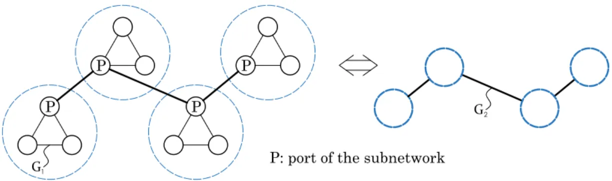
1.1 An illustration of the proposed model for a network of networks, where the subnetworks over graph G1 are interconnected via their port nodes

(desig-nated with letter P) over graph G2. . . 27

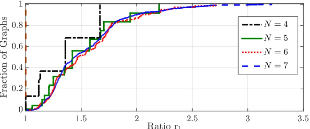
1.2 The fraction of connected unweighted graphs for which the ratio r1 is less than a threshold (see Example 1.8.2) . . . 31

1.3 Performance asymptotic over paths in continuance of Example 1.6.1. . . . 35

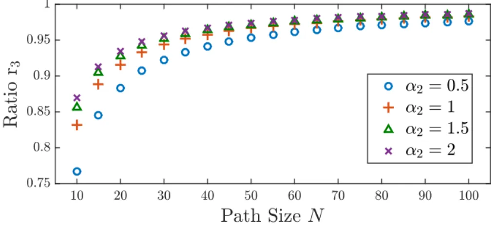
1.4 Ratio r₃ for a network of harmonic oscillators over a path graph as the net-work size grows (see the continuance of Example 1.6.4) . . . 35

1.5 Schematic of the composite network whose performance is analyzed in the continuance of Example 1.7.4 . . . 36

1.6 The formation of interest in Example 1.9.1 . . . 38

1.7 The performance functions for Example 1.9.1 . . . 38

1.8 The sample outputs based on the designs in Example 1.9.1 . . . 39

2.1 This plot shows the sparsity pattern of the original graph versus the sparsified graph (the self-loops are more visible in the colored version). . . 81

2.2 The ratio of eigenvalues of the sparsified Laplacian to the eigenvalues of original Laplacian. The dashed the top and bottom dashed lines depict the expected bounds of this ratio, 1 +and 1−. . . 81

2.3 Experimental distribution of the performance measure of the multi-agent system with sparisified graph Laplacian produced in Example 2.8.3, for single, double, and triple integrators from left to right. . . 83

(16)

2.5 The optimal values of performance measure for different values of N and γ. 85 2.6 The mean of optimal values of the entries of feedback gainKfor the

platoon-ing dynamics. The variance (for different values ofN) is relatively negligible in this scale, so we have omitted error-bars on the data points. . . 86 2.7 The performance measure before and after reweighting . . . 88 2.8 The performance measure versus number of iterations. . . 88 2.9 A sample representation of the degrees of the graph between the agents after

the reweighting procedure. . . 89 2.10 An illustration from the optimal weights of the links in the case ofN = 351.

The grounded nodes are denoted by black color, and are spaced by 5 vehicles. 89 3.1 A schematic of two topologies for a random network. . . 98 3.2 The sample output of the noisy networks with fixed and random graphs. . . 99 3.3 The performance measure and its bounds for Example 3.5.6. . . 104 3.4 The underlying graphs of the network in Example 3.5.7 . . . 106 3.5 These colored plots show the performance measure and its lower-bound

com-puted for π1, π2∈[0,1], whereπ1+π2+π3 = 1. . . 106

3.6 The lower-bound compared to the value of performance measure derived from MC method, together with the machine times. . . 107 3.7 The mean time of the computations versus number of the nodesn(the lower

figure magnifies the details of the upper figure) . . . 108 3.8 Representation of an optimal vector of probabilities Π for a network with

m= 100 underlying graphs. . . 109 3.9 Representation of a sparse optimal Π with reweighted`1 penalization, where

more entries are on the horizontal axis. . . 109 3.10 The Performance Loss and Density Level tradeoff illustrated by increasing

the value ofγ (see Example 3.6.6). . . 110 4.1 The performance measure of the network of two agents in Example 4.4.7 with

(17)

4.2 The performance measure of the Kuramoto model of two agents in Example 4.4.8 with the parameter K. . . 140 4.3 The performance measure of nonlinear consensus network withα= 0.25 and

the graph at the linearized Laplacian of complete graph. . . 150 4.4 The performance measure of nonlinear consensus network with N = 8, α =

0.25 and random graphs with different number of edges . . . 150 5.1 The worst case relative performance degradation based on the bound of

The-orem 5.7.6. . . 176 5.2 The spatial location of subsystems and their coupling structure. . . 182 5.3 The space-time representation of the sampling strategies corresponding to

frame Φ and sparsified frame Φs, with|Φ|= 1760 and |Φs|= 503. . . 182 5.4 The histogram of the performance degradation after random partitioning. . 183 5.5 The space-time representation of the sampling points of the sequence of

frames Φ1, . . . ,Φ12 that are separated by the dashed lines. . . 184

5.6 The estimation measure of the sparsified frames resulting from Algorithm 6 (the randomized sparsification) and Algorithm 5 (the greedy sparsification) are compared. . . 185 5.7 The estimation measure of the shifted frames is compared to our theoretical

upper bound (5.22). . . 185 6.1 A sample illustration of the observation times in classic least-squares observer

(dashed blue lines) and an arbitrary observation strategy (black solid lines). 202 6.2 Space-time representation of the switching observation strategy (black lines)

created by the sparsification of the observation strategy corresponding to the classical estimator (dashed blue lines) (see Example 6.7.1). . . 216 6.3 Empirical cdf for the estimation measure after sparsification using Algorithm

(18)

7.1 The schematic of the motion and vision model adopted in this chapter at three consecutive snapshots. The location of the robot is denoted by letter R, which moves and changes its orientation across three frames. The features are denoted by letter f. As a result of this movement, the visible features (those in between the dashed lines) in each frame will vary. Set Θtwill consist of all features that can be triangulated during this horizon. . . 231 7.2 The top view of the navigation environment. The 3D reference curve is seen

as a circle from this view. . . 237 7.3 A snapshot of the environment. The blue pyramid demonstrates the camera’s

field of view. The features that are inside the frame at this time are high-lighted. The deformed 8-shaped curve is the reference path as parametrized in (7.36) (see Fig. 7.2 for the top view as well). The robot is also rotating according to (7.38). . . 238 7.4 The estimation measure values resulting from three method. The curves

corresponding to the to the greedy method and the proposed method may not be distinguished in this plot. . . 238 7.5 The RMS error in the positions of the robot resulting from feature selection

using different methods. The curces corresponding to the greedy method and Algorithm 1 may not be distinguished in this plot. . . 239 7.6 Comparison of the RMS error resulting from the uniform random method and

our proposed approach with the greedy method. This plot shows a speed-up by almost an order of magnitude in the feature selection using Algorithm 7. 242 7.7 The empirical CDF’s for parameters κt and κut, which show the ratio of

the spent CPU time for the random sampling (including all independent 50 experiments) to the greedy method. The plot show that in this example the random sampling is faster than the greedy method by almost an order of magnitude. . . 242

(19)

8.1 An example showing how the spatial variables dictate the observations of agents. The observations by 3 agents at two consecutive time instants have been magnified. This highlights the need for a communication mechanism and temporal memories. . . 255 8.2 The diagram illustrating the essence of our framework. . . 263 8.3 The testing accuracy for different frame sizes f and time horizons T versus

the number of training epochs. . . 266 8.4 Average maximum testing accuracy versus frame size f and time horizon

T after 30 epochs with random walks (top figure). In the middle one, we trained extra 20 training epochs for the motion planning policy. The last figure illustrates the error reduction as a result of the design of coordination policy instead of random walks. . . 272 8.5 A sample of masked images created by putting together the observations by

3 different agents for a time horizon of T = 3 with f = 8. This image is the input to the centralized image classifier as an alternative classification approach (method (i)). The (random) uncovered parts have been reached due to random walks. . . 273 8.6 Comparison of the testing error when using a centralized method with the

suggested approach. The first 20 epochs of training corresponds to the case for random walks, while in the next 20 epochs we optimize the movements of the agents. . . 273 8.7 The result of training when with and without communications. . . 274 8.8 The training results for different number of agents. . . 274 8.9 Visualization of the learned communications strategies and how they share

their beliefs with each other using t-SNE plots. . . 275 9.1 Snapshots of the proposed problem at the beginning of three episodes. The

blue and green squares point to the current position of the agent and the goal of each episode. During each episode, the agent has moved towards the goal. . . 279

(20)

9.2 A schematic diagram of the 3-layered deep learning architecture for goal gen-erator, action planner, and classifier. The dots correspond to repeating the preceding modules forrtimes. In the planners, the number of channels in the convolutional filters is fixed and equal todin the consecutive layers. For the classification module, the number of output channels from the convolutions is doubled each time. Thus, in each case we will have different numbers of intermediate channelsqg,qa, andqc(the components are not drawn). . . . 280 9.3 We demonstrate six sample trajectories from two data points. The snapshots

have been taken at the beginning of 4 episodes as well as the end of the last episode. The blue and green squares point to the current position and goal position. The prediction corresponding to the final unmasked image is also illustrated in each case. . . 289 9.4 The confusion matrix of classification computed on the test dataset. The

reported numbers are averaged over 20 runs of data. . . 290 9.5 The testing data accuracy vs. data epoch using the hierarchical training

sequence from scratch. . . 290 9.6 Testing data accuracy vs. data epoch with transfer learning. . . 290

(21)

Abstract

In this dissertation, we consider a range of different problems in systems, control, and learning theory and practice. In Part I, we look at problems in control of complex networks. In Chapter 1, we consider the performance analysis of a class of linear noisy dynamical systems. In Chapter 2, we look at the optimal design problems for these networks. In Chapter 3, we consider dynamical networks where interactions between the networks occur randomly in time. And in the last chapter of this part, in Chapter 4, we look at dynamical networks wherein coupling between the subsystems (or agents) changes nonlinearly based on the difference between the state of the subsystems. In Part II, we consider estimation problems wherein we deal with a large body of variables (i.e., at large scale). This part starts with Chapter 5, in which we consider the problem of sampling from a dynamical network in space and time for initial state recovery. In Chapter 6, we consider a similar problem with the difference that the observations instead of point samples become continuous observations that happen in Lebesgue measurable observations. In Chapter 7, we consider an estimation problem in which the location of a robot during the navigation is estimated using the information of a large number of surrounding features and we would like to select the most informative features using an efficient algorithm. In Part III, we look at active perception problems, which are approached using reinforcement learning techniques. This part starts with Chapter 8, in which we tackle the problem of multi-agent reinforcement learning where the agents communicate and classify as a team. In Chapter 9, we consider a single agent version of the same problem, wherein a layered architecture replaces the architectures of the previous chapter. Then, we use reinforcement learning to design the meta-layer (to select goals), action-layer (to select local actions), and perception-layer (to conduct classification).

(22)

Part I:

Control Problems in Complex

Networked Systems

(23)

Chapter 1

Performance Analysis of Noisy

Dynamical Networks

1.1 Introduction

Developing tools to reduce design complexity has been in the center of recent research in networked control systems [1–5]. In several important applications, network design problem reduces to finding an optimal communication (graph) topology among a network of identical subsystems that are coupled to each other through some common mission-related control objectives. Examples include formation control in a cooperative team of robots [6], the platoon of vehicles in automated highways [7], space-time rendezvous in a team of robots, and networks of synchronous oscillators in power networks. In fact, the recent jumps in the underlying technology have ignited several applications of these ideas [8, 9].

Here we bring a brief history of the origins of research in this field. From a control the-oretic perspective, Tsitsiklis pioneered in systematically looking at the machinery required to tackle the decentralized coordination of the agents [10]. The relationship between this notion and the concept of consensus became more clear later. The seminal paper by Fax and Murray [11] is one of the earliest endeavors in the modern control that highlighted the connection of consensus problem to the Laplacian matrix of the underlying graph. Two significant extensions were carried out by Jadbabaie et. al. [12] and Olfati-Saber and

(24)

Mur-ray [13, 14], where the simple connectivity assumptions for the graph of the network were relaxed. These pieces have been either a foundation or inspiration for contributions in dif-ferent directions. For instance, the consensus over random networks [15, 16] or time-varying topologies [17], rendezvous using proximity graphs [18], consensus of double-integrators [19], or with self-triggered communications [20] are a fraction of ideas that were followed by the community.

The design problem usually involves the optimization of a measure of performance or robustness while respecting various constraints. Due to their combinatorial nature, most network design problems become intractable as network size increases and suffer from high computational complexities. Possibility of characterizing performance and robustness mea-sures in closed and explicit forms will significantly facilitate the design process by allowing the network designer to identify relevant functional properties of the measures and their behaviors with respect to the interconnection topology. In this chapter, we present ex-plicit expressions for the H2-norm, as a performance and robustness measure, of a class of

interconnected network of linear control systems.

The authors of [21] consider coherency of a platoon of vehicles by evaluating the H₂ -norm of second-order consensus algorithms and propose several scaling laws for various scenarios of coordination. In [22], ill-posedness of a certain class of platoons is investigated and shown that stabilizability deteriorates as the size of the platoon increases. The string stability of a class of formation problems with limited communication range is studied in [23], where a fundamental limit on the disturbance rejection quality of the network in the frequency domain is derived. The stability and robustness of large platoon of vehicles with double-integrator dynamics are considered in [24], where it is shown that how scaling of a robustness measure (in terms of the platoon size) to external disturbances improves from geometric to polynomial growth when vehicles are allowed to communicate with their two immediate neighbors. In [25], robustness analysis and distributedH∞controller design of platoon of vehicles with third-order models and undirected communication topologies are considered. In [26], several graph theoretic bounds on the H2-based performance of

linear consensus networks with first- and second-order dynamics are characterized and it is shown how the performance measure scales with the network size and depends on structural

(25)

properties of the communication topology. In [27], the authors consider distributedH₂ and H∞ controller design for a multi-agent system whose subsystems have general linear time-invariant dynamics. Using a consensus-like algorithm and notion of the grounded graph (e.g., see [28]) to model coupling of agents to leaders, it is shown under what conditions such controllers exist and how they can be suboptimally designed.

In this Chapter, we consider a network of identical subsystems that are connected over an undirected graph and subject to external disturbance and measurement noise. We propose a methodology to express the steady-state variance of the output of a class of intercon-nected linear time-invariant networks as a rational function of their Laplacian eigenvalues. Our method extends the existing results in the literature for first- and second-order linear consensus network models (cf. [2] and reference in there). We illustrate that the notion of minimum connectivity threshold is useful for the design of the feedback gains for these networks. It turns out that stabilizability of the nodal dynamics (and detectability in case of observer-based output-feedback) guarantee the existence of such designs. Using these developments, it is shown that fundamental limits may emerge for networks whose subsys-tems are non-minimum phase. We find graph-theoretic bounds for the performance of the network, which paves the way to find scaling laws for the performance measure. Moreover, a tradeoff between the graph sparsity and performance measure is revealed. Additionally, for networks over path or cycle graphs, we find the asymptotic trend of the performance measure. We bring two extensions of the analyses for the cases of observer-based output feedback as well as a class of composite networks. We have included several parametric and numerical examples to support our theoretical contributions. Our approach is advantageous for the design of these dynamical networks. Our spectral expressions can facilitate solv-ing of underlysolv-ing optimal control problems: instead of dealsolv-ing directly with optimization problems with high-dimensional matrices, our method leverages the structure of the control system and decouples the roles of typically low-dimensional feedback gains and the eigen-spectrum of the communication graph. The proofs and additional details of the examples of this chapter are included in the appendix.

(26)

1.2 Notations and Preliminaries

Here we bring the notations and preliminaries used throughout this chapter. Most of these notations are adapted in the upcoming chapters as well.

The sets of real and integer numbers are denoted byRandZ, respectively. The+and++

subscripts denote the nonnegative and positive subsets of a set, respectively (e.g. R+). Tr(.)

represents matrix trace. The partial ordering on the cone of positive-semidefinite matrices is denoted viaand similar operators. The standard basis forRN is denoted by{e1, . . . , eN}. The vector and matrix of ones are denoted by 1N ∈RN andJN ∈RN×N, respectively. Also,

IN andMN =IN −JN/N are identity and centering matrices, respectively. The centering matrix subtracts the average of a vector from every element; i.e., for any vectorx∈_RN_{, it} holds that MNx = x− 1 N N X i=1 xi ! 1N. (1.1)

The vectorization is denoted by vec(S). The Kronecker product is denoted by A⊗B. The matrix transpose and conjugate transpose are denoted by (.)T and (.)∗ superscripts, respectively. A weighted undirected graph overN nodes is a collectionG= (V,E, k), with a set of nodes V ={1,2, . . . , N}, a set of edgesE ⊂

{i, j}:i, j∈ V}, and a weight function k : E → _R+. We define kij := k({i, j}) =kji and form the (symmetric) graph Laplacian

L= [lij]∈RN×N with entries lij =        X {i,j}∈E kij ifi=j −kij ifi6=j . (1.2)

The set of neighbors of a node is Ni :=

j∈ V

{i, j} ∈ E for i∈ V. The eigenvalues of

L are denoted byλ1 ≤ · · · ≤λN, which are real and nonnegative for a weighted undirected graph. For a connected graph, λ1 = 0 with eigenvector 1N, and λ2 > 0. The Laplacian

eigendecomposition is L=UΛUT_,_where_U _{is its orthonormal matrix of eigenvectors and}

Λ= diag(λ1, . . . , λN).

(27)

behavior, consider the following notations.

qn=O(pn) if qn/pn≤C for someC >0.

qn=O(pn)⇔pn= Ω(qn).

qn=O(pn), qn= Ω(pn)⇔qn= Θ(pn).

qn∼pn⇔ lim

n→∞qn/pn= 1.

1.3 Problem Statement

We consider an interconnected network of N subsystems where the dynamics of the i’th subsystem are governed by

Si:            ˙ xi(t) = Axi(t) +Bui(t) +Eξi(t) yi(t) = Hxi(t) +σ ηi(t) zi(t) = Cxi(t), , (1.3)

for i = 1, . . . , N, in which xi(t) ∈ Rn is the state vector of the subsystem, ui(t) ∈ Rp is the control input, ξi(t) ∈ Rm1 is an exogenous disturbance input, ηi(t) ∈ Rm3 is the measurement noise,yi(t)∈Rqis the measurable output, andzi(t)∈Rm2 is the performance output. The matrices A ∈_Rn×n_,_B _∈

Rn×p, C∈Rm2×n, E∈ Rn×m1, and H ∈Rq×n are fixed known matrices. Parameter σ ≥0 dictates the magnitude of the measurement noise compared to the disturbance process. The state of the entire network is

x(t) :=x1(t)T, x2(t)T, . . . , xN(t)T T

∈RN n.

The vectors representing the network input, disturbance, feedback noise, feedback output, and controlled output are similarly defined and denoted byu,ξ,η,y, and z, respectively.

(28)

con-sensus), i.e., to fulfil the goal

xi(t)−xj(t)→0 as t→ ∞

for alli, j∈ {1, . . . , N}. To realize this objective, we employ the following feedback control law ui(t) =− X j∈Ni Kij yi(t)−yj(t) (1.4)

for each subsystem i∈ {1, . . . , N}. The subsystems are allowed to exchange their relative output measurements information over an undirected communication graphG. It is assumed that the structure of the feedback gain matrices Kij ∈Rp×q are restricted to

Kij =kijK

where kij’s are nonnegative scalars (i.e., the weights of graphG) and K ∈ Rptimesq is the common factor among all feedback gain matrices.

When stabilizing feedback control law (1.4) exists and there is no exogenous noise, i.e.,

E=0 and σ = 0, one can show that xi(t)−xj(t)→0 as t→ ∞ holds for the closed-loop network. However, in the presence of noise, the state variables will fluctuate around the consensus state. Let us quantify these fluctuations. First, note that the deviation from the average of state of a subsystems is

νi(t) := zi(t)− 1 N N X j=1 zi(t) (1.5)

for every node i∈ V. We can represent (1.5) in vector form as

ν(t) = (MN ⊗Im1)z(t) = (MN ⊗C)x(t), (1.6)

where MN is the centering matrix of size N. We inspect that the network (1.3) with control law (1.4) asymptotically reaches consensusif and only if vector of deviations from

(29)

the average ν(t) asymptotically goes to zero. Since control law (1.4) can be rewritten as

u(t) =−(L⊗KH)x(t), (1.7)

the controller synthesis breaks into two components: designing a feedback gain K and designing a weighted undirected graph with LaplacianL. It is assumed that measurement noise and disturbance are both Gaussian, uncorrelated, and with independent components with unit variance.In order to measure the aggregate fluctuations in the network, we adopt the steady-state variance of the deviation from the average as a measure of performance for the design, which is defined by

ρ(L,K) := lim t→∞E

kν(t)k2₂ . (1.8)

Theresearch problems are to characterize performance measure (1.8) in terms of Lapla-cian eigenvalues of the underlying communication graph of the network, illustrate role of feedback (and observer) gains in stability and emergence of fundamental limits on perfor-mance measure and design tradeoffs, and derive scaling laws for the perforperfor-mance as the network grows.

1.4 Stability and Performance Measure Characterization

We look at the stability criteria for these dynamical networks. Moreover, we derive and characterize spectral expressions for the performance measure. For brevity, we remove the time argument from the variables in the rest of this chapter.

Once we apply feedback control protocol (1.4), the closed-loop dynamics of the state of the network are given by

˙

(30)

We define auxiliary variables r,χ, andγ to be

r:= (UT ⊗In)x, χ:= (UT ⊗Im1)ξ, x, γ := (U

T _⊗_I

m3)η. (1.10)

Then, the following dynamical decoupling is realized (see [27] for the case of state-feedback without the measurement noise).

Proposition 1.4.1. By the change of variables (1.10), the resulting closed-loop network dynamics given by (1.9) are decoupled into N systems

Σi : r˙_i = (A−λ_iBKH)r_i+Eχ_i−λ_iBKσγ_i, (1.11)

for each i = 1,2, . . . , N. In the absence of disturbance and noise, the network reaches consensus if and only if systems Σ2, . . . ,ΣN are asymptotically stable.

We leverage this decoupling to arrive at spectral expressions for the performance measure of the network.

Theorem 1.4.2. Suppose that in (1.11) systems Σ2, . . . ,ΣN are asymptotically stable. Then, the performance measure can be expressed as

ρ(L,K) = N X

i=2

φ(λi,K), (1.12)

with the performance functionφ(λ,K) given by

φ(λ,K) := Tr CP(λ,K)CT

, (1.13)

which is a rational function ofλand entries ofK. The mapP(λ,K) is the unique positive-definite solution to an algebraic Lyapunov equation given by

(A−λBKH)P(λ,K) +P(λ,K)(A−λBKH)T +EET +λ2σ2BK(BK)T =0, (1.14)

(31)

The dimension of the dynamics of each subsystem is often small and has nothing to do with the number of subsystems. Therefore, evaluation of performance functionφ(λ,K) can be done via symbolically solving Lyapunov equation (1.14) after converting it to a linear system by vectorization (see the proof of Theorem 1.4.2).

Due to linearity of the Lyapunov equation in termsEET+λ2σ2BK(BK)T one inspects that the performance functionφ can be decomposed into two components according to

φ(λ,K) =φξ(λ,K) +σ2φη(λ,K),

in which spectral functionsφξandφη only reflect the effect of disturbance and measurement noise, respectively.

Remark 1. In this Chapter, we occasionally skip argument Kin φ(λ,K) and denote it as φ(λ). In those cases, we solely consider the dependence of the functions on the eigenvalues of the graph Laplacian (i.e., for a fixed feedback gain K).

Remark 2. A part of the result of Theorem 1.4.2 is hidden in the analysis provided in [27], in the case of state-feedback. However, the authors did not explicitly derive the spectral expressions for the performance.

1.4.1 Extension of Stability Analysis to Observer Design

We extend the previous analysis to the output-feedback and synthesize a decentralized observer. We show that the separation principal in the linear filtering using Luenberger observers is naturally carried into this design as well.

Our procedure consists of four steps:

(i) We augment the dynamics of subsystem i by an observer variable ˆxi ∈ Rn, whose dynamics are governed by

˙ˆ

xi=Axˆi+Bui+ ˆui, (1.15)

where ˆui ∈Rn is an auxiliary control input for the observer. We will set the value of this input in a decentralized manner in the last step.

(32)

(ii) As it is usual in the observer design, we use ˆxi to compute

ui =−Kxˆi. (1.16)

(iii) In addition to the relative output feedback onHxi, the subsystems should share the value of Hxˆi with their neighbors. Once we consider these three steps, the augmented dynamics of subsystem iare given by

ˆ Si :                                       ˙ xi ˙ˆ xi   =    A −BK 0 A−BK       xi ˆ xi   +    0 In   uˆi+    E 0   ξi ˆ yi =    H 0 0 H       xi ˆ xi   +    Im3 0   ηi zi= C 0    xi ˆ xi    , (1.17)

Variable ˆyi has the same role as yi in (1.3); i.e., the augmented subsystems will use the relative-feedback on this variable.

(iv)We use the following theorem and design the gain of control law (1.4) when applied on subsystems ˆSi in (1.17), which in this case will be an observer gain.

Theorem 1.4.3. Suppose that we apply control law (1.4) on augmented subsystems Sˆi in (1.17) by setting ˆ ui =−Fˆ X j∈Ni aij(ˆyi−yˆj), (1.18)

where the observer gain is set to be

ˆ

F=

−F, F

∈_Rn×(2q)_. _(1.19)

Moreover, assume thatF∈_Rn×q_{is chosen such that} _A₋_λ

iFHis Hurwitz fori= 2, . . . , N. Then, the estimation and regulation are separated: if we apply control input ui given in

(33)

based relative output-feedback reaches the consensus in the absence of disturbance and noise. For this design, we denote the resulting performance function byφ(λ,K,F). This func-tion can be found similar to the case of simple state-feedback, except that we need the augmented matrices of ˆSi given in (1.17) for solving (1.14) and evaluation of this function. Remark 3. Note that the separation principal only holds in the stability analysis. The resulting performance functions φ(λ,K,F) may not be decomposed into functions that only depend on one of gainsKorF.

The separation principal together with the duality between the estimation and regulation let us prove similar results for the quality of estimation using this decentralized observer. We now elaborate. First, we define the error of estimation using this observer as

e(t) := ˆx(t)−x(t). (1.20)

Because we are only employing the relative feedback, we may only control the deviations of the error components from their average. These deviations are reflected by the variable

δ(t) := (MN ⊗In)e(t). (1.21)

Next, we define the estimation measure for network as

µ(L,F) := lim t→∞E

kδ(t)k2

2 . (1.22)

The dual of system Σi in (1.11) is

Υi : r˙i = (A−λiFH)ri+Eχi−λiσFγi , (1.23)

which lets us deduce the next result (compare to Theorem 1.4.2).

(34)

Then, we can express the estimation measure as µ(L,F) = N X i=2 ψ(λi,K), (1.24)

with the estimation functionψ(λ,K) given by

ψ(λ,K) := Tr (Q(λ,K)), (1.25)

which is a rational function ofλand entries ofF. The map Q(λ,K)is the unique positive-definite solution to an algebraic Lyapunov equation given by

(A−λFH)Q(λ,K) +Q(λ,K)(A−λFH)T +EET +λ2σ2FTF= 0, (1.26)

for all values of λthat make A−λFHa Hurwitz matrix.

Remark 4. In [29], the authors propose the following alternative observer-based approach. They define their observer variable vi to follow the dynamics

˙

vi =Fvi+Gyi+TBui, (1.27)

and define their control law as

ui=KQ1 N X i=1 aij(yi−yj) +KQ2 N X i=1 aij(vi−vj), (1.28)

where matrixFhas no eigenvalue in common withA, the pair (F,G) is stabilizable, andT

is the unique solution to Sylvester equationTA−FT=GC. Then, they designK,Q1 and

Q2 such that a design with minimum connectivity threshold is achieved. One can see that

our design is different and simpler as we only need a feedback gainKand an observer gain

F. Moreover, our approach is built upon the separation principle between the regulation and estimation, which is also the case in the classical Luenberger (or LQG) observer design. Therefore, unlike our approach, It is not evident how the separation principal shows up in their design.

(35)

1.5 Design of Control Law Gains

We investigate the problem of finding feedback gains and focus on gains inducing a minimum connectivity threshold. This property makes the design process with respect to the graph more tractable. After that, we discuss related performance limitations.

1.5.1 Minimum Connectivity Threshold

We define the minimum connectivity threshold ˜λ(K)∈[0,∞] for a feedback gain K to be

˜

λ(K) := inf λ>0

λ: (A−cBKH) is Hurwitz for c > λ . (1.29)

Similar notions have been reported (e.g. [27]), while our goal is characterization of conditions for finding gains with ˜λ(K)<∞1_{. The following definition is for this purpose.}

Definition 1.5.1. The feedback gain K is said to have an unbounded stability region if ˜

λ(K)∈[0,∞).

If K has an unbounded stability region, then the network is robust to all increases in the connectivity: if the network is output-stable for a given graph G1 with Laplacian L1,

then for every graphG₂ with LaplacianL2 and G1⊂ G2, the network is still output-stable.

The reason is that λi(L1) ≤ λi(L2) for i= 2, . . . , N (this has been emphasized in [27] as

well). Moreover, this makes the stability analysis with respect to the graph more tractable, since ensuringλ2(L)>λ(˜ K) guarantees the output-stability of network. Before bringing

methods to find such feedback gains, let us look at a consequence of choosing them.

Theorem 1.5.2. For a network designed with a feedback gain K that in endowed by a

connectivity threshold λ(˜ K) < ∞, the performance function φ(λ) is analytic on interval (˜λ(K),∞).

The openness of the interval of interest in Theorem 1.5.2 suggests that if ˜λ(K) > 0, we need to maintain a minimum distance from this value. This will make sure that the stability margin is large enough.

1_˜

(36)

1.5.2 State-Feedback Minimum Connectivity Design

Let us consider the state-feedback (i.e.,H=Inin (1.3)). It turns out that the stabilizability is the necessary and sufficient condition for existence a gain K that induces a bounded threshold ˜λ(K).

Theorem 1.5.3. If (A,B) is stabilizable, then for every value of c > 0, the choice of feedback gain given by

K= 1

2B

T_Q−1_, _(1.30)

satisfies λ(˜ K) ∈ [0, c], where Q 0 is a solution to the following feasible linear matrix inequality.

AQ+QAT −cBBT ≺0. (1.31)

Conversely, if there exists a gain K withλ(˜ K)<∞, then (A,B) is stabilizable.

The linear matrix inequality (LMI) (1.31) is a computational tool to find a gain K

for a given network and graph with a minimum connectivity threshold at most equal to c (see Example 1.9.1). The solvability of LMI (1.31) is called the quadratic stabilizability of (A,B) by means of a linear state-feedback (see Section 7.2 of [30]).

Remark 5. This result is inspired by Theorem 11 in [27], while our main contribution is to clarify the role of stabilizability in existence of feedback gains with minimum connectivity threshold.

Remark 6. The optimality in choice of Q is not the concern in Theorem 1.5.3. Instead, we focus on the existence of designs for K with a minimum connectivity design. In fact, various performance criteria could potentially get addressed. For instance, suppose that for

somed >0, we replace LMI (1.31) with

(37)

˜

λ(K) ≤ c, but also for each eigenvalue λ > ˜λ(K), the poles of A−λBK have real parts

less than−d(see [31]). As another example, authors of [27] brought a version of the matrix inequality which ensures that each decoupled subsystem ΣihasH2-norm less than a desired

value, which they state that could be conservative in practice. Criteria such as robustness or non-fragility could be potentially added by building on top of (1.31) as well (e.g. see [32]).

1.5.3 Observer-Based Minimum Connectivity Design for Output-Feedback The duality between the derived conditions onA−λiFHin Theorem 1.4.3 and onA−λiBK in Theorem 1.5.3 lets us conclude the following result that resembles the result of Theorem 1.5.3.

Theorem 1.5.4. Suppose that (A,H) is detectable. Then, for every c > 0, the following observer gain for the settings of Theorem 1.4.3, has an unbounded stability region with ˜ λ(F)∈[0, c]. ˆ F= −1 2Q −1_HT_, 1 2Q −1_HT ∈Rn×(2q), (1.33)

where Q0 is a solution to the following feasible LMI.

ATQ+QA−cHTH≺0. (1.34)

Conversely, if under the settings of Theorem 4 an observer gainFhas a boundedλ(˜ F), then (A,H) is detectable.

The LMI (1.34) is the quadratic stabilizability condition for the dual pair (AT,HT) (it is stabilizable since (A,H) is detectable).

1.5.4 Asymptotic Performance and Estimation Bounds

An important design question is if the performance functionφ(λ,K) can be made arbitrarily small, which is related to the notion of almost disturbance decoupling [33]: attenuating the effect of the disturbance in a performance metric as much as desired. We study the case of relative state-feedback below.

(38)

Theorem 1.5.5. Suppose that(A,B)is stabilizable and(A,C)is detectable and thatσ = 0. For all pairs of λ > 0 and K for which A−λBK is Hurwitz, the performance function resulting from the relative state-feedback is bounded from below according to

φ(λ,K)>TrETP0E

, (1.35)

for a positive semi-definite matrixP0 given by

P0 := lim

→0P (1.36)

where P is the unique positive semi-definite solution to the parametric algebraic Riccati equation

ATP+PA+CTC−−2PBBTP=0. (1.37)

Matrix P0 is zero if and only if transfer matrix C(sIn −A)−1B is right-invertible and minimum-phase.

For instance, if the transfer matrix is C(sIn−A)−1B non minimum-phase and the columns of E are not in the null space ofP0, then the bound in (1.35) is strictly positive.

The dual of this result for estimation quality is given below, whose proof is identical to Theorem 1.5.5 and has been omitted.

Theorem 1.5.6. Suppose that (A,E) is stabilizable and (A,H) is detectable. If for some gain F, A−λiFHare Hurwitz for i= 2, . . . , N, then

ψ(λ,F)>Tr(S0),

for a positive semi-definite matrixS0 given by

S0 := lim

σ→0Sσ, (1.38)

(39)

equation

ASσ+SσAT +EET −σ−2SσHTHSσ =0; (1.39)

Matrix S0 is zero if and only if transfer matrix H(sIn−A)−1E is right-invertible and minimum-phase.

1.5.5 Parametric Evaluation of λ˜(K)

In both relative state or output feedback designs, if n is not large (e.g. n ∼ 1 to 4), we may design K with an unbounded stability region using Routh-Hurwitz criteria and explicitly evaluate ˜λ(K). In fact, the characteristic equation of the matrixA−λBKHfor the decoupled systems for eigenvalue λis

pλ(s) =p(s;λ,K) = det (sIn−(A−λBKH)). (1.40)

They must be Hurwitz polynomials forλ=λ2, . . . , λN. As we enforce the Routh-Hurwitz criteria, we find a set of essentially nonlinear inequalities involving λ and elements of K, such that the minimum connectivity threshold is realizable and evaluable based on values of K(see the next section for examples).

1.6 Examples of Performance Analysis

In this section, before bringing more theoretical contributions, we bring different classes of subsystems and characterize their performance within this framework. Note that more details from these examples have been provided in Appendix Q. In many examples in this chapter, we are interested in convexity of the performance functions. This is due to the fact that this property would let us derive graph theoretic performance bounds for the network (see Section 1.8).

First, we consider two single-input single-output controllable subsystems under the rel-ative state-feedback, where the disturbance and control input drive the dynamics from the same channel (without the measurement noise).

(40)

Realization φ(λ,K) s1: A=−a, B=E= 1, C= 1 1 2(kλ+a) s2: A= 0 1 −a2 −a1 B=E=0 1T C= [b1 b0] b2 0k1λ+a2b20+b21 2(k2λ+a1)(k1λ+a2)

Table 1.1: The subsystems investigated in Example 1.6.1 together with the performance functions in the case of relative state-feedback with σ= 0. We assume thata, a1, a2 ≥0.

Example 1.6.1. Consider the subsystems given in Table 1.1, where we have also reported the corresponding performance functions. For the nodal dynamics s1 and s2, supposing

that K=k >0 and K= [k1, k2]0, respectively, in both cases ˜λ(K) = 0. Moreover, for

λ >λ(˜ K), performance function φ(λ) is strictly convex and strictly decreasing. If all ai’s

are zero andC=eT

1, these subsystems are called single and double-integrators, respectively.

As a numerical example, let us consider double-integrators with k1 =k2 = 1. Then, using

the second row of Table 1.1 we get

φ(λ) = 1

2λ2. (1.41)

This is a well-known result (e.g. see [34]).

Example 1.6.2. Consider double-integrators with relative feedback only on positions; i.e.,

H= [1,0].

We use the decentralized observer of Theorem 1.5.4. We let K= [k1, k2] 0 and set the

observer gain to be F= [f1, f2]T. Theorem 1.4.3 requires the stability analysis for matrix

A−λFH, which is Hurwitz if and only if f1, f2 >0. Then, we get ˜λ(F) = 0. We can show

that φ(λ,K,F) = c1λ 4₊_c 2λ3+c3λ2+c4λ+c5 c6λ4+c7λ3+c8λ2 , (1.42)

(41)

wherec1 toc8 are polynomials ofk1, k2, f1,andf2. Using the observer withk1 =k2=f1=

f2 = 1, (1.42) becomes

φ(λ) = 9λ

4_{+ 11λ}3_{+ 9λ}2_{+ 4λ}_{+ 1}

6λ4_{+ 2λ}2 . (1.43)

One observes that for weak connectivity regimes (i.e., λnear zero), φ(λ) in (1.43) is close to the function in (1.41), while as λ increases, the performance function corresponding to relative state-feedback vanishes, while the function from observer design does not.

Example 1.6.3. We consider a triple-integrator subsystem with dynamics

...

xi=ui+ξi. (1.44)

Let us choose the state to be [xi,x˙i,x¨i]T with element-wise positive gainK= [k1, k2, k3]0.

We can show that

φ(λ,K) = k3

2(k1k2k3λ2−k21λ)

, λ(˜ K) = k1 k2k3

. (1.45)

The next two examples also have performance functions that under conditions become strictly decreasing and convex.

Example 1.6.4. The dynamics of a harmonic oscillator of massm are governed by

¨ xi =−2ζω0x˙i−ω02xi+ ui m + ξi m, (1.46)

where ζ is the damping ratio and ω0 is the undamped angular frequency (see [35]). We

consider C= [1,0] and computeφ(λ) with the relative state-feedback on [x,x]˙ T _with _K₌ [k1, k2] 0. Using arguments similar to Example 1.6.1, if we define α1 := mω02/k1 and

α2 := 2mω0ζ/k2 we get the performance function

φ(λ,K) = 1

2k1k2(λ+α1) (λ+α2)

. (1.47)

(42)

decreas-ing forλ >˜λ(K) = 0.

Example1.6.5 (Platoon of Vehicles). We consider a network of vehicles, in which the position

of i’th vehicle is denoted bypi∈R. It has the third-order dynamics

τ...p_i+ ¨pi =ui+ξi, (1.48)

where the inputui ∈Ris the desired acceleration and ξi ∈Ris the disturbance. The time-constantτ > 0 characterizes how fast the vehicles responds to the acceleration command. The state vector is chosen as [pi,p˙i,p¨i]T, where they denote the (errors in) the position, velocity, and acceleration of the vehicles in the platoon, respectively (see [25] for more details). The state-space matrices are given in the appendix. Using relative state-feedback, by application of the Routh-Hurwitz criteria we find that ifK= [k1, k2, k3] satisfiesk1, k2>

0, k3 ≥0,we get ˜ λ(K) =      0 ifk3 = 0 max 0,τ k1−k2 k2k3 ifk3 >0 . (1.49)

We can show that ifσ = 0, we get

φ(λ,K) = 1

2k1k2

k3λ+ 1

k3λ3+ (k2−k1τ)λ2/k2

. (1.50)

If k3 = 0, the design corresponds to a relative output-feedback on only positions and

velocities, with a performance function

φ(λ) = 1

2k1(k2−k1τ)λ2

,

which is strictly convex and strictly decreasing for λ > ˜λ(K) = 0. If k3 >0, we have the

(43)

Example 1.6.6. Consider a network with nodal matrices A=    0 1 0 0   , B=    0 1   , C= −ζ 1 ,

forζ > 0 and σ = 0. We observer that the subsystems have a non minimum-phase

input-output transfer function

C(sI2−A)−1B=

s−ζ

s2 ,

whereζ >0 is the location of the right-hand plane zero. Let us consider the relative state-feedback. We can show that in this case, we have P0 = diag (2ζ,0). For a disturbance

matrixE= [α, β]T, Theorem 1.5.5 gives us the bound

φ(λ,K)>Tr ETP0E

= 2ζα2. (1.51)

Alternatively, if we use the relative state-feedback, we can show that the corresponding performance function φ(λ,K) is

α2(k1+k2ζ)2λ2+ (2k1α2ζ2+ 2k2αβζ2+k1β2)λ+β2ζ2

2k1k2λ2

,

which is strictly convex and decreasing for λ > ˜λ(K) = 0. Now, for any gain K with an unbounded stability region

lim λ→∞φ(λ,K) = α2(k1+k2ζ)2 2k1k2 =α2(1 +rζ) 2 2r , (1.52)

where r := k2/k1. By differentiation with respect to r, we find that the right side attains

its minimum atr= 1/ζ. Thus

φ(λ,K)> lim

λ→∞φ(λ,K)|k2/k1=1/ζ = 2ζα

2_, _(1.53)

which is the same bound as (1.51). The bound on the performance function scales with the magnitude of the right-hand plane zero at ζ. One inspects that if the disturbance enters

(44)

the subsystem from the same channel as the control input, we do not face a fundamental limitation on the performance, because in this case it does not touch the zero dynamics of the subsystems (see [36] for a similar observation in the case ofH∞-norm).

Example 1.6.7. In this example, first, we consider two different designs for a network of double-integrator agents with measurement noise. Recall that the magnitude of feedback noises is controlled by parameter σ >0.

(i)the relative state-feedback without the filtering (i.e., without the decentralized observer): in this case, usingK= [k1, k2], we can show that

φ(λ,K) = 1 k1k2λ2 +σ2k 2 1 +k22 2k1k2 , (1.54)

in which the first term can be recovered from Table 1.1 and the second term appears due to the measurement noises.

(ii) the relative output-feedback on positions with the decentralized observer: in this case

φ(λ) =φξ(λ,K) +σ2

c9λ2+c10λ+c11

c12λ2+c13λ+c14

, (1.55)

in which φξ is the performance function read from (1.42) and c9 toc14 are polynomials of

ki’s andfi’s. For instance, in the case ofk1 =k2 =f1=f2= 1, this function becomes

φ(λ) = 9λ

4_{+ 11λ}3_{+ 9λ}2_{+ 4λ}_{+ 1}

2(3λ2_{+ 1)} +σ

26λ2+ 5λ+ 1

2(3λ2_{+ 1)} . (1.56)

Next, we find estimation function ψ(λ,F). We can show that

ψ(λ,F) = 1 2f1f2λ2 +σ 2 2 f1λ+ f2 f1 . (1.57)

The first term is due to the disturbances, while the second term originates from the feedback noises. The transfer matrixH(sI−A)−1Eis right-invertible and minimum-phase. Hence, as Theorem 1.5.6 suggests, as noise densityσ shrinks, one can make the estimation arbitrarily precise by increasing the magnitude of observer gainsf1 and f2.

(45)

1.7 Analysis of Network of Networks

We introduce and analyze a class of networks of networks that are built by a repeated application of control law (1.4). For simplicity of the developments, we neglect the feedback noises (i.e., set σ = 0). One can show that the same approach works in the presence of those noises as well.

1.7.1 Construction Procedure for Composite Networks

First, we build identical networks using control law (1.4) over graph G₁. We denote the number of nodes ofG1 by mand the order of the state-space realization for each subsystem

byn. Moreover, we denote the feedback gain used to build each network byK1∈Rp×q. Let

us denote the state of the subsystem j in module or subnetwork iby x(_ji) ∈Rn. Similarly, we denote the rest of corresponding variables. The Laplacian matrix corresponding to G1

is also denoted by L1. For the subsequent analysis, let us define the following matrices

˜

A:=Im⊗A−L1⊗BK1H, B˜ :=em⊗B, (1.58) ˜

E:=Im⊗E, C˜ :=Im⊗C, H˜ :=eTm⊗H.

According to (1.9), the dynamics of the subnetwork iare given by

˙ x(i)= ˜Ax(i)+ ˜Eξ(i), (1.59) wherex(i):= (x(₁i))T . . . (x(mi))T T

∈_Rmn_,_{is the state vector of module} _i_{and disturbance} vector ξ(i) ∈ _Rmm1 _{is defined similarly. Without loss of generality, we designate the last}

node in graph G₁ as the port of the module2, which corresponds to a subsystem that we can add a term to its control input. This converts (1.59) to new open-loop dynamics

˙

x(i) = ˜Ax(i)+ ˜Bu(i)+ ˜Eξ(i), (1.60)

2

(46)

whereinu(i)∈_Rm _{is a tunable control input to the module. Moreover, we assume that two} modules can become interconnected only through their port nodes. Then, the only variable that moduleican use for relative feedback is the output variable for the port node, which is denoted by

y(i)= ˜Hx(i)=Hx(_mi). (1.61)

We collectN instances of these networks with dynamics (1.60) and feedback variables (1.61) to construct a composite network. Therefore, the subsystems equivalent to Si in (1.3) for this network design are

S(i):            ˙ x(i) = ˜Ax(i)+ ˜Bu(i)+ ˜Eξ(i) y(i) = ˜Hx(i) z(i) = ˜Cx(i) , (1.62)

with the structured matrices defined by (1.58). Now, we build a modular network by application of control law (1.4) with N modules (or subnetworks) connected over a higher level graph G2 with feedbackK2 ∈Rp×q. 3 If{i, j} ∈ E2 has a weight denoted bybij, then the application of control law (1.4) will be

u(i)=−K2 X {i,j}∈E2 bij y_m(i)−y_m(j) . (1.63)

We have N modules and each one consists of m subsystems. Therefore, the consensus output of the entire network should be

νnn(t) := (MN m⊗C)x(t). (1.64)

Then, we set its steady-state variance as the performance measure

ρnn(L2,K2) := lim

t→∞E

kνnn(t)k22 , (1.65)

3 _{Feedback gains}_K

1 and K2 are matrices of the same dimension because we have chosen one node as

(47)

P

P P

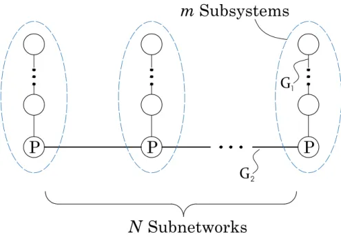
P

G1

G2

P: port of the subnetwork

Figure 1.1: An illustration of the proposed model for a network of networks, where the subnetworks over graph G1 are interconnected via their port nodes (designated with letter

P) over graphG₂.

whereL2 is the graph Laplacian of G2.

In Fig. 1.1, we illustrate this composite structure using an example: we have four modules and inside each of them, three subsystems are interconnected over graph G₁, in this case a complete graph. These subnetworks are then connected via their ports over another graphG2, which in this case is a path graph.

Interpretation of Construction: Let say modules (or subnetworks) iand j are connected, thus {i, j} ∈ E2. Then, the ports of these two modules will have access to the relative

difference of their feedback output ym(i) −y(mj) and will reflect this feedback term in their control input. Mathematically speaking, the input to the port node4 _{in module} _i_is

u(_mi)=−K1 X {m,k}∈E1 amk y_m(i)−y(_ki) (1.66) −K2 X {i,j}∈E2 bij y_m(i)−y(_mj).

The first term is due to initial application of control law (1.4) over G1 with an edge set E1,

while the second term isu(i) from (1.63) based on the composite network design over G2.

1.7.2 Stability and Performance of Composite Networks

Theorem 1.7.1. Consider a dynamical network over graphG1 with a bounded performance

measureρ(L1,K1). Suppose that in Proposition 1 and Theorem 1 we apply control law (1.4)

(48)

on systems S(i) defined in (1.62) over G₂ with feedback gain K2. The resulting composite

network reaches consensus if and only if A˜ −λi(L2) ˜BK2H˜ is Hurwitz for nonzero

eigen-values of L2. Moreover, if φnn(λ,K) is the performance function derived from Theorem 1

for subsystemsS(i) defined in (1.62), then

ρnn(L2,K2) =ρ(L1,K1) +

N X

i=2

φnn(λi(L2),K2). (1.67)

The significance of this result is that for a fixed module graph G1 with Laplacian L1

and K1, the value of ρ(L1,K1) and the form of composite performance function φnn are

fixed. Thus, we can quantify the role of higher level graph G2 and feedback gain K2 in

the performance of the composite network by looking at the second term. The extra term compared to Theorem 1.4.2 appears because

νnn = (MN m⊗C)x6=

MN ⊗C˜

x, (1.68)

where the right-hand side is the output that would have resulted in an expression of form (1.12).

Remark 7. If a subnetwork is one subsystem, then (1.67) reduces to (1.12), since each subsystem as a network satisfiesρ(L1,K1) = 0.

1.7.3 Minimum Connectivity Design For Composite Networks

We show that if ˜λ(K1) < ∞, then there exists a simple choice for K2 such that it has

also an unbounded stability region in terms of the eigenvalues of higher level LaplacianL2;

i.e., ˜λ(K2) exists and ifλ >λ(˜ K2) then ˜A−λBK˜ 2H˜ is Hurwitz. This would remedy the

concerns about possible complexities in the design ofK2 over graph G2 .

Theorem 1.7.2. Suppose that the subnetworks are built over any graph G1 and feedback

gainK1, which has an unbounded stability region. For anyα >0, let us choose the feedback

gain of the composite network to beK2 =αK1. Then, K2 has an unbounded stability region

(49)

Dynamics Performance Functionφnn(λ) single-integrator 2(m−1)λ+m 2 2mkλ double-integrator (m−1)(m+ 2)λ 2_{+ 2}_m2₍_m₋₁₎_λ₊_m4 2m2_k 1k2λ2

Table 1.2: Performance functions for a composite network with complete graph subnetworks of single and double-integrator agents. Each module has m nodes and the feedback gains are assumed to be identical over both graphs (see Example 1.7.5).

Corollary 1.7.3. Suppose that the subnetworks of the network of networks are built with

K1, which induces ˜λ(K1) = 0. Let us choose K2 =αK1 for some α > 0 in the design of

the described composite networks. Then, higher level feedback gain K2 satisfies ˜λ(K2) = 0

with respect to the eigenvalues of higher level Laplacian L2.

1.7.4 Examples of Networks of Networks

Example 1.7.4. Consider a modular network with subnetworks of single-integrators over an unweighted path graph G₁ of m nodes, where the last node of the module is its port. We choose K1 = k1 > 0, so the open-loop dynamics of the modules before design of the

composite network based on (1.60) are

˙

x(i)=−k1L1x(i)+emu(i)+Imξ(i), (1.69)

where x(i) ∈ _Rm_{, ξ}(i) _∈

Rm, u(i) ∈ R, and L1 is Laplacian of the unweighted path graph

over m nodes. Then, choosing K2 = k2 > 0, the performance function of the composite

network is

φnn(λ) =

(m(m−1)/2)k2λ+k1m

2k1k2λ

. (1.70)

Based on Corollary 1.7.3 in the higher level ˜λ(K2) = 0. Moreover, we inspect that the

resulting family of functions is strictly convex and decreasing for λ >0 (see the appendix for the details).

Problems in Control, Estimation, and Learning in Complex Robotic Systems

Lehigh Preserve

Lehigh Preserve

Problems in Control, Estimation, and Learning in Complex Robotic

Problems in Control, Estimation, and Learning in Complex Robotic

Systems

Systems

Problems in Control, Estimation, and Learning in

Complex Robotic Systems

by

Hossein K. Mousavi

(Officially, SeyyedHossein Mousavi)

Presented to the Graduate and Research Committee of

Lehigh University

in Candidacy for the Degree of

Doctor of Philosophy

in

Mechanical Engineering

Lehigh University

January 2020

Acknowledgements

Contents

List of Tables

List of Figures

Abstract

Part I:

Control Problems in Complex

Networked Systems

Chapter 1

Performance Analysis of Noisy

Dynamical Networks

1.1

Introduction

1.2

Notations and Preliminaries

1.3

Problem Statement

1.4

Stability and Performance Measure Characterization

1.5

Design of Control Law Gains

1.6

Examples of Performance Analysis

1.7

Analysis of Network of Networks