R E S E A R C H A R T I C L E
Open Access
Sparse Proteomics Analysis – a
compressed sensing-based approach for
feature selection and classification of
high-dimensional proteomics mass
spectrometry data
Tim O. F. Conrad
1,5*, Martin Genzel
2, Nada Cvetkovic
1, Niklas Wulkow
1, Alexander Leichtle
3,
Jan Vybiral
4, Gitta Kutyniok
2and Christof Schütte
1,5Abstract
Background: High-throughput proteomics techniques, such as mass spectrometry (MS)-based approaches, produce very high-dimensional data-sets. In a clinical setting one is often interested in how mass spectra differ between patients of different classes, for example spectra from healthy patients vs. spectra from patients having a particular disease. Machine learning algorithms are needed to (a) identify these discriminating features and (b) classify unknown spectra based on this feature set. Since the acquired data is usually noisy, the algorithms should be robust against noise and outliers, while the identified feature set should be as small as possible.
Results: We present a new algorithm,Sparse Proteomics Analysis(SPA), based on the theory of compressed sensing that allows us to identify a minimal discriminating set of features from mass spectrometry data-sets. We show (1) how our method performs on artificial and real-world data-sets, (2) that its performance is competitive with standard (and widely used) algorithms for analyzing proteomics data, and (3) that it is robust against random and systematic noise. We further demonstrate the applicability of our algorithm to two previously published clinical data-sets.
Keywords: Machine learning, Feature selection, Classification, Compressed sensing, Sparsity, Proteomics, Mass spectrometry, Clinical data, Biomarker
Background
During the last decade, high-throughput assays systems1 for measuring a variety of different biological sources have become standard in modern laboratories. This allows for the quick and cheap creation of very large data-sets which characterize for example the status of a cell by its bil-lions of constituents, e.g. nucleotides, RNAs, contained proteins, or metabolites. Ideally, analyzing these massive data-sets leads to a better understanding of the under-lying biological processes. Especially in the context of *Correspondence: [email protected]
1Department of Mathematics, Freie Universität Berlin, Arnimallee 6, Berlin,
Germany
5Zuse Institute Berlin, Takustr. 7, Berlin, Germany
Full list of author information is available at the end of the article
characterizing—and ultimately understanding—diseases, a first step is often to find significant differences in the data between samples from healthy and diseased indi-viduals. There are many successful examples where this approach based on -omics data (e.g., genomics, pro-teomics, or metabolomics) led to the identification of biological markers, enabling a new type of molecular diag-nostics. We call a collection of biological markers that represents the differences on the data level a disease fingerprint.
Many disease-relevant mechanisms are controlled by proteins (e.g. hormones), which can be detected in biolog-ical samples (blood, urine, etc.) usingmass spectrometry (MS). This technique allows (potentially) for monitoring the entire set of proteins—the so-called proteome—in © The Author(s). 2017Open AccessThis article is distributed under the terms of the Creative Commons Attribution 4.0 International License (http://creativecommons.org/licenses/by/4.0/), which permits unrestricted use, distribution, and reproduction in any medium, provided you give appropriate credit to the original author(s) and the source, provide a link to the Creative Commons license, and indicate if changes were made. The Creative Commons Public Domain Dedication waiver (http://creativecommons.org/publicdomain/zero/1.0/) applies to the data made available in this article, unless otherwise stated.
a given sample. Due to its wide availability in hospi-tals, MS-based proteomics can bring the next wave of progress in diagnostics, since even subtle changes in the proteome can be detected and linked to disease onset and progression [1–4].
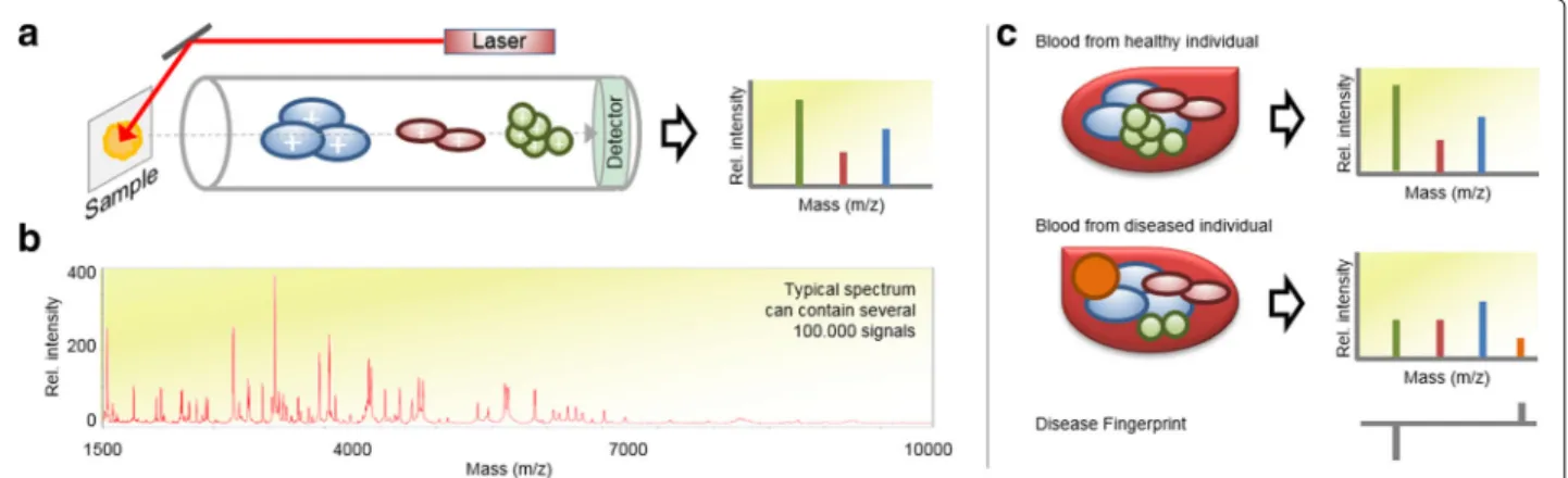
Disease fingerprints:The main idea of the identifica-tion ofdisease fingerprintsusing MS-based proteomics is sketched in Fig. 1:
(a) A mass spectrum is generated reflecting the consti-tution of a given (blood-)sample with respect to contained molecules. (b) Based on mass spectra from two sample groups (representing a healthy control group and a group having a particular disease) differences are detected. This set of differences precisely corresponds to adisease fin-gerprint, since it represents a trace caused by a particular disease in the proteome. Several studies have shown that this approach works well in practice and found differences do indeed reflect correlations between changes in the mass spectrum, the proteome, and phenotypic changes ([5–9]). Panels of proteomic markers (fingerprints) have been shown to be more sensitive and specific than con-ventionally biomarker approaches [2], for example when diagnosing cancer [10–12]. However, a single proteomics data-set can contain tens of millions of signals which is many orders of magnitudes larger than the number of available observations in a typical study.
Our ultimate goal is therefore to build a library of pro-teomics disease fingerprints which are extracted from high-throughput MS experiments. These would enable to diagnose diseases based on their proteomic fingerprints— just by analyzing an individual’s proteome. Ideally, these fingerprints are of low-complexity allowing easy interpre-tation by experts, e.g. medical doctors, and the imple-mentation of medical assays for routine diagnostics, e.g. in an hospital environment. Clearly, the less components
an assay is composed of, the easier it is to implement and interpret.
Thus, a fingerprint should only consist of a minimal col-lection of proteins specific for a particular disease and should be robust against noisy measurements. On the other hand, the acquired data from the high-throughput experiments is very high-dimensional and contains large amounts of random and systematic noise which makes an automatic analysis of mass spectra a very challenging task. Hence, the discovery of biomarkers is still a widely open research topic and there are several analytic problems that hinder reproduction of results (see [13] for example).
Despite these challenges there is indeed hope that these disease specific, low-complexity fingerprints exist: It has been shown for several cancer types that a small num-bers of genes and proteins can be identified that serve as biomarkers (e.g. for lung cancer [14], breast cancer [15] or pancreas cancer [16]). This means that only a few sig-nals in a mass spectrum can be used to derive a sparse classifier.
MS1 data:In this work we consider mass spectrometry (MS) data acquired from a standard MALDI-TOF instru-ment because it is easy to obtain using comparatively cheap MS-instruments which are widely available, e.g. in hospitals. Opposed to other approaches such as tandem mass spectrometry (MS/MS), we directly work on the raw data acquired inprofile modeand do not aim for identi-fication. Thus, each mass spectrum (sample) always has the same number ofd dimensions (number of entries).2 Recall, that the entries in a mass spectrum are a weight-ordered list of ion-counts of the respective ion-masses. (See also Fig. 1.)
One of the reasons for this is that standard approaches for MS data analysis usually convert the MS data to peak lists as a first step and work on the converted data.
Fig. 1 aSchematic outline of a linear matrix-assisted laser desorption ionization (MALDI)–time-of-flight (TOF) mass spectrometer (MS). During the measurement process, the molecules of the examined sample are ionized, vaporized and finally analyzed by their respective time-of-flight through an electric field. This process generates a plot (mass spectrum) having mass-to-charge ratio (m/z) on thex-axis and intensity (ion count) on the y-axis.bTypical mass spectrum for a mass range of 1500–10.000 Dalton.cExample of a disease fingerprint, created by comparing mass spectra from a healthy and a diseased individual
However, signals can be missed by this conversion step due to noise or missing values in the raw data which hin-ders peak detection. Opposed to this, our approach does not rely on any peak identification but works on the raw data. This allows for a more robust analysis in presence of noise which is a typical challenge in MS data analysis.
Problem definition
In this article, we will focus on the following problem setting:
We assume that we are given data of n mass spectra derived fromn biological samples (e.g. from blood of n individual patients) in form ofnpairs{(xi,yi)}i=1...n. Here,
xi ∈ Rd represents the mass spectrum of the i-th
sam-ple (e.g. thei-th patient) andyi ∈ {−1,+1}its respective
class, e.g., healthy or diseased. Thus, eachxi(representing
an individual mass spectrum) containsdentries.
The goal is to identify a (small) set of features, i.e. indices in the mass spectrum, separating these two classes. Thus, a feature represents a specific position (or mass) in a mass spectrum in which the two groups (e.g. healthy vs. diseased) differ. This corresponds to the well known prob-lem offeature selection3and leads to a potential disease fingerprint for the given data.
Mathematically, this can be formulated as the identifi-cation of afeature vectorω0= (ω0,1,. . .,ω0,d)∈Rdsuch
that4
yi=signfω0(xi) for “many” samples i=1,. . .,n,
(1) with alinear decision function fω0(xi):=ω0,xi=dj=1ω0,jxi,j.
From a geometric perspective, this means that the hyperplane with normal vectorω0appropriately separates the data-points of the respective classes.
This means that ω0 can be used as a linear classifier where each entry ofω0corresponds to a specific position in a spectrum and the non-zero entries (which we call fea-tures) indicate their significance. Our goal is therefore to learn a sparseω0for which Eqn. 1 holds. As a particular consequence, a classifier based on suchω0will yield good prediction accuracy.
In most realistic scenarios for feature selection, unfor-tunately, the number of features is much larger than avail-able samples (d n) and the data suffers from noisy measurements. For these reasons, the number of feasi-ble classifiersω0can become extremely large, so that the problem ofoverfittingcan occur. In order to allow inter-pretability and generalization of the classifier, it is in fact inevitable to restrict the solution space for ω0. In this paper, we focus on verysparse5vectorsω
0satisfying (1), which precisely reflects our wish for a minimal disease fingerprint.
At this point, it should be emphasized that (1) does not need to hold forallsamples but rather for most of them. Allowing for such a small “mismatch” in the model, we incorporate the crucial fact that a simple binary output model, such as (1), might describe the disease label only with high accuracy but not necessarily exactly. In turn, this asks for a certain robustness of the used method against wrong predictions with regard to (1).
We will approach this challenge by formulating the fea-ture selection problem as a constrained (or regularized) optimization problem: min ω∈Rd n i=1 Lyi,fω(xi) subject to R(ω)≤λ, (2)
whereL: R×R→Ris aloss(error) function,R:R→R is aregularization(cost) function that encourages a par-ticular structure ofω (e.g., sparsity), and the parameter λ ≥ 0 controls the degree of model complexity. Given any potential feature vectorωand the (true) output label y, the loss functionL(y,fω(x))measures the discrepancy between the actual and the desired prediction.
As already pointed out, we are particularly interested in a method that producesoptimal and robust solutionsin the following situation:
• The input data(x,y)are noisy,
• the number of data dimensionsd is large (typically:
d=105. . .108),
• the number of samplesn is relatively small (typically:
n=102. . .104), and
• the set of highly-relevant features is small (i.e., a minimal disease fingerprint indeed exists), which corresponds to a small number of non-zero elements inω0(typically:#{i|ω0,i =0} 100).
On the contrary, we are not mainly interested in the methods’ overall classification performance. Measures of classification performance such as accuracy are indicators whether a learned classifier accurately separates the data into classes. In our case, we assume that the data can be characterized well by asparseclassifierω0whose non-zero entries are those used for classification and are therefore of medical relevance. That means, ifω0is sparse and leads to good classification accuracy then only a few entries contribute and medical interpretation becomes feasible. However, if there does not exists a sparse ω0 such that Eq. 1 holds, there is strong evidence that no sparse (sim-ple) characterization is possible. This indicates that the underlying biological mechanisms are too complex to be captured by a sparse (simple) model. If this is the case, every sparsity-encouraging method will fail, meaning that a sparse classifier will always give poor classification. As a consequence, an important assumption of this work is that a sparseω0(ground-truth) exists.
As we will see later it is often possible to find non-sparse classifiers which achieve better classification accu-racy. This might be favorable in some situations in which the main focus is indeed on overall classification accu-racy. However, in these situations overfitting becomes an issue and the identification of interpretable, highly-discriminative features might be extremely difficult. In the context of MS-data analysis such a classifier would be especially hard to interpret because of the very high dimensionality of the data.
State of the art in sparse feature selection
There are numerous approaches for feature selection which mainly fall into three categories:
• Filters: Using some score or correlation function (e.g., based on Fisher’s, t-test, information theoretic criteria) evaluating the importance of each feature in aunivariate way and taking the top-rated features.
• Wrappers: Using machine-learning algorithms to evaluate and choose features using some search strategy (e.g. simulated annealing or genetic algorithms).
• Embedded methods: Selecting variables by directly optimizing an objective function (usually in a multivariate way) with respect to: goodness-of-fit and (optionally) number of features. This could be achieved with algorithms like least-square regression, support vector machines (SVM), or decision trees.
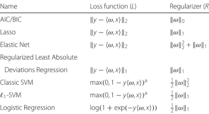
In this paper, we will mainly focus onembedded methods. Regarding this category, the literature contains several well-known options for choosing combinations of loss and regularization functions (cf. (2)), some of which are exemplarily listed in Table 1.
Table 1Prominent options for choosing loss function and regularizer in feature extraction algorithms
Name Loss function (L) Regularizer (R)
AIC/BIC y− ω,x2 ω0
Lasso y− ω,x2 ω1
Elastic Net y− ω,x2 ω22+ω1
Regularized Least Absolute
Deviations Regression y− ω,x1 ω1
Classic SVM max(0, 1−yω,x)a 1
2ω22
1-SVM max(0, 1−yω,x)a 12ω1
Logistic Regression log(1+exp(−yω,x)) 1
2ω1
*This is the so calledHinge loss
The1- and2-norm of a vectorz=(z1,. . .,zd)∈Rdare defined by z1=dj=1|zi|andz2=(dj=1|zi|2)1/2, respectively. The “0-norm”z0, simply counts the number of non-zero entries ofz
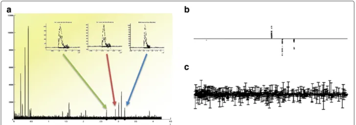
Different combinations can influence the results dra-matically: Fig. 2 demonstrates the effect of sparsity by comparing a2- and1-regularized version.
In this example, a proteomics data-set was created that contains three discriminant features between the two sub-groups. It can be easily seen how the results differ: While the 1-based result is optimized for selecting only a few features, the2-variant selects much more features which in turn results in a better fit of the observation model. In this paper, we are interested in developing a method that selects as few features as possible while achieving the best possible fit under this constraint. This is in contrast to methods that aim at only achieving the best possible fit. A low-complexity model is of particular interest in biolog-ical applications because each selected feature is usually analyzed in subsequent experiments, which creates addi-tional costs.
Various approaches can be used to assess the outcomeω of a feature selection method, when appropriate training and test data are available. We will use the following three measures of quality: (i) correctness of the selected fea-tures, (ii) size of the selected feature set, (iii) performance of classifying an unknown test set (specificity, sensitivity, accuracy). Obviously, (i) can only be used if the correct features are known, which is the case in our benchmark data-sets (for more details see “Feature selection from simulated data-sets” section).
Contribution
As already mentioned above, the major challenge of sparse feature extraction is to robustly identify asmallset of vari-ables (non-zero components of ω) that can be used to accurately classify unknown proteomics data (e.g. healthy or diseased) according to (1). This paper introducesSparse Proteomics Analysis(SPA), a novel framework for feature selection and classification. The key step of our method is based on1-bit compressed sensing(cf. “Compressed sens-ing-based data analysis” section) and solves the following optimization problem:6 max ω∈Rd n i=1 yixi,ω subject to ω1≤ √ λandω2≤1, (3) where the regularization is now defined by two inequality constraints on the feature vectorω.7The above approach is motivated by the general theory of compressed sens-ing, which was originally introduced by Donoho as well as by Candès, Romberg, and Tao (cf. [17–19]) and pro-vides a modern framework for efficiently acquiring and processing high-dimensional (nearly) sparse signals (for more details see “Compressed sensing-based data analy-sis” section).
Fig. 2 aOverlaid spectra from two different groups. The three peaks marked by thearrows(magnified in the inlays) represent the underlying differences between the two groups.bSparseωfound by a1-regularized method (1-SVM).cωfound by2-regularized method (classical SVM)
We shall verify the competitiveness of our method by applying it to several synthetic and real-world data-sets and comparing the results to those of other widely-used algorithms in this field. Although the core of the algorithm (3) is surprisingly simple, we will observe that SPA (includ-ing pre- and postprocess(includ-ing steps) finds optimal feature vectors which are extremely sparse, allow for highly accu-rate classification, and are robust against noise. In particu-lar, for “very-sparse” situations, it even turns out that SPA outperforms the standard methods listed in Table 1.
Note that computational solutions to (2) or (3) are usually based on solving a convex program by standard optimization techniques, such as interior point meth-ods. However, these methods sometimes scale poorly with increasing number of samples n and data dimensiond, as it is typically the case for -omics data analysis. Several strategies have been proposed in the literature to speed up the calculations, e.g., using stochastic decent ([20–24]). In this article, we shall not focus on such computational issues but rather on providing a novel way of formalizing and solving the feature selection problem, namely in the context of compressed sensing.
Apart from the specific approach of (3), it is a general concern of this work to promote the benefit of sparse embedded methods. In contrast to classical (univariate) approaches, such as statistical tests, the process of vari-able selection takes place in an automatic fashion here. In this way, a costly preprocessing (e.g., peak detection) as well as subsequent feature assessments can be avoided as much as possible. Especially in a situation where only a very few samples are available, those additional steps may cause further instability and their success strongly relies on the specific data structure. In fact, it was already succinctly emphasized by Vapnik in ([25], p. 12) that“If you possess a restricted amount of information for solving
some problem, try to solve the problem directly and never solve the more general problem as an intermediate step. It is possible that the available information is sufficient for a direct solution but is insufficient for solving a more general intermediate problem.” This fundamental princi-ple is precisely reflected by our viewpoint, which only makes a few (generic) assumptions on the underlying data model. Finally, we would like to mention that recently, rigorous theoretical guarantees for sparse feature selec-tion from MS data were shown in [26]. Using the novel idea ofoptimal problem representations, the mathemati-cal framework of [26] even goes beyond the binary output scheme of (1) and allows for a unified treatment of general observation and data models.
The next sections shortly review the background of compressed sensing and then describe our novel feature selection approach SPA in detail (“Methods” section). Finally, we present several benchmark results in “Feature selection from simulated data-sets” sections and “Results for real-world MALDI-TOF MS data” for simulated and real data-sets and compare them to current state-of-the-art algorithms.
Compressed sensing-based data analysis
In its most simple form, compressed sensing (CS) stud-ies the recovery of an unknown vector x ∈ Rd from linear measurements y = Ax. Here, A ∈ Rn×d is an (n × d)-matrix and the entries of y ∈ Rn contain the
measurements. The major challenge is now to design the measurement processAin such a way that the number of measurementsnis as small as possible and, at the same time, x is still (uniquely) recoverable fromy. Thus, we are asking for the maximalcompressibility ofxby linear measurements.
Obviously, when n d, we require some additional information to obtain a unique solution ofy = Ax. The prior information on x which is studied in compressed sensing is the assumption ofsparsity, i.e., most coefficients ofx are assumed to be zero, or at least very small. One naive approach to incorporate this additional property is to search for the sparsest solution ofAz=y:8
arg min
z∈Rd
z0 subject to Az=y. (4)
Unfortunately, this problem is non-convex and cannot be efficiently solved in general. Therefore, one usually replaces (4) by itsconvex relaxation, which is also known as thebasis pursuit([27]):
arg min
z∈Rd
z1 subject to Az=y. (5)
One of the first key results in compressed sensing states that, if A ∈ Rn×d is chosen randomly, e.g., with inde-pendent and identically distributed Gaussian entries, and n = O(s·log(d/s)), then (with “high probability”) every s-sparse vector x(i.e.,x0 ≤ s) can be uniquely recov-ered from (5). The most surprising fact is that the number of required measurementsn = O(s·log(d/s))only log-arithmically depends on the (possibly large) dimension d of the ambient space. Hence, random measurement processes indeed allow for a very strong compression of sparse vectors (see also [17–19] for more details).
In order to consider more complicated situations, the stability and robustness of the basis pursuit algo-rithm was extensively studied. Various theoretical results and numerical experiments show that this algorithmic approach can also be applied for the stable recovery of vectors which are only nearly sparse, as well as to noisy measurements of the form y = Ax + η. To obtain a robust version of (5), one may replace its equal-ity constraint by Az − y2 ≤ for some appro-priate noise level > 0. Not very surprisingly, this approach is also closely related to the Lasso introduced by Tibshirani in [28] (see also (2) and Table 1).
1-bit compressed sensing
In many practical scenarios, especially when working with computers, there is no way to represent real numbers exactly. Thus, it is reasonable to assume that the measure-ment vectorAxis acquired in aquantized(and therefore non-linear) fashion. The most extreme form directly leads to1-bit measurements, i.e., only the signs ofAxare known:
yi=sign(ai,x), i=1,. . .,n, (6)
wherea1,. . .,an ∈ Rd are the rows of the measurement
matrixA∈Rn×d. As in classical compressed sensing, we
are asking for an appropriate recovery ofxfrom (6) using
as few measurements as possible. This challenge was orig-inally considered in [29] as1-bit compressed sensing, and has been extensively studied in [30, 31].
A surprisingly simple convex recovery approach was proposed by Plan and Vershynin in [31]:
max z∈Rd n i=1 yiai,z subject toz1≤ √ λandz2≤1, (7) where λ > 0 denotes the sparsity-controlling param-eter. To get some intuition, we first note that we have yi =sign(ai,x)if and only ifyiai,x >0 holds. Hence,
maximizing the sum in (7) will ensure the consistency of many measurements i ∈ {1,. . .,n}, according to (6). However, the total consistency is not enforced so that (7) indeed allows for noisy inputsythat do not satisfy (6). On the other hand, the constraint of (7) promotes sparsity of the final outcome. To see this, we may consider the set Sd,λ:= {z∈Rd:z0≤λ,z2≤1}and observe that (cf. [31] Sec. III)9
conv(Sd,λ)⊂{z∈Rd:z1≤
√
λ,z2≤1} ⊂2conv(Sd,λ). This means that (7) optimizes over a convex relaxation of the setSd,λ which contains allλ-sparse vectors in the unit ball. For more details, see also [31]. The main state-ment of [31] proves that the robust 1-bit compressed sensing algorithm (7) indeed allows for an appropriate recovery of sparse vectors, using onlyn=O(λ·log(d/λ)) measurements. Moreover, it is surprisingly robust against several types of noise, including (random) bit-flips of the labels.
RemarkThe minimized functional of (7) is closely related to the hinge loss which is used for SVMs (cf. Table1). Indeed, without rejecting the negative part of the hinge loss, we would precisely end up with the objective functional in(7).
The constraint of (7), on the other hand, can be regarded as a combined1-2-condition, where the tuning parame-terλcontrols the desired level of sparsity of the minimizer. This type of regularization strongly resembles the idea of elastic nets, originally proposed by Zou and Hastie in[32].
Why compressed sensing?
At a first sight, the main challenges of compressed sens-ing and machine learnsens-ing (ML) seem to be very different. In compressed sensing, we intend to design a measure-ment processAin order tocompressa vectorx, whereas in machine learning, the training data is already contained in the rows ofAand we are rather willing toexplainthe observationsyby some appropriate vectorx. However, in both areas we are asking for a (sparse) recovery from a cer-tain type of measurement. Indeed, alinear regressionin
ML exactly corresponds to classical CS model (see “Com-pressed sensing-based data analysis” subsection), and a classification problem is actually equivalent to 1-bit CS (see “1-bit compressed sensing” subsection).
Therefore, it is not very surprising that the applied algorithms for compressed sensing and machine learn-ing resemble each other, and that theoretical results in both fields rely on the same mathematical foundations (concentration of measure, convex geometry, etc.). Unfor-tunately, both communities only rarely interacted with each other. In this paper, we would like to emphasize the viewpoint of compressed sensing, in particular, because it is still not very common for the classification tasks that we deal with.
With the recent progress in compressed sensing and related areas as low-rank matrix recovery or quantized CS, also new algorithms like nuclear norm minimization or 1-bit CS have been proposed. Although these meth-ods are typically motivated by theoretical studies, they perform also very well for real-world data. In general, we believe that these alternative perspectives allow for deeper theoretical insights, finally leading to the improvement of the classical (1-based) tools from machine learning.
For an extensive introduction to compressed sensing, we refer to [33, 34]. As we already mentioned above, compar-ing this text to literature from statistical learncompar-ing theory (see [35] for example), the reader will quickly notice many interesting connections between both fields.
Methods
In this section, we present the details of our novel frame-work which we callSparse Proteomics Analysis (SPA). It is based on the ideas of 1-bit compressed sensing presented in the previous section. The first part provides a math-ematical formulation of the feature selection problem as well as a brief overview of the steps that are performed in SPA. The rest of this section is then devoted to a detailed description and discussion of the single steps.
Setting and overview
As already mentioned in the introduction, we assume that our learning process is supervised, i.e., we know which spectrum belongs to the class of healthy (yi = +1) and
diseased (yi = −1) samples in advance. If the data
vec-torsxi ∈ Rd,i = 1,. . .,nare mass spectra, the indices
j= 1,. . .,dofxi=(xi,1,. . .,xi,d)correspond to them/
z-values10and its entries represent the intensities. The non-zero entries of the feature vectorω0 = (ω0,1,. . .,ω0,d) ∈
Rddescribe the location of the disease fingerprints and its
respective values the significance of these features. In the setting of classical learning theory, we are ask-ing for a hyperplane{ω0}⊥which correctly separates most of the data points xi labeled by yi. More precisely, this
means11
yi=sign(xi,ω0) for “many” samples i=1,. . .,n. (8) Equivalently, we can view (8) as a problem from 1-bit com-pressed sensing (cf. “Why comcom-pressed sensing?” section), i.e., we have acquired noisy 1-bit measurements and are now looking for a sparse recovery.
In the development of SPA, we have primarily focused on the latter perspective, and therefore, the 1-bit recovery program (7) forms the key step of our algorithm:
Algorithm 1(SPA at a glance). Input:Raw data samples{(xi,yi)}i=1,...,n
Output:Sparse feature vectorω˜ ∈Rd
Preprocessing:
1: Normalize data to make the spectra comparable. 2: Perform smoothing by a convolution with Gaussian
density.
3: Standardize data.
Sparse Feature Selection:
4: Perform 1-bit CS optimization (7) to find feature vectorωˆ.
Postprocessing:
5: Detect the connected components ofωˆ to obtain a sparsified versionω˜.
6: (Optional) Reduce dimension by projecting data onto the feature space.
Algorithmic details
In the following, we are going to specify and discuss the single steps of Algorithm 1.
Step 1: normalization of the data
This step heavily depends on the underlying acquisition method of the data. Every spectrumxi∈Rdis normalized
by a certain scaling factorμi > 0, i.e.,xi →μixi fori =
1,. . .,n. The individual scalarsμishould be chosen such
that the resulting data vectors are “comparable.”
For example, when we assume that the data are acquired by MALDI-TOF-MS as described in Fig. 1, it seems to be quite natural to normalize them by the total ion count. Mathematically, this means that we would divide every spectrum by its1-norm, i.e., we chooseμi =1/xi1.
Step 2: smoothing by gaussian density
We already pointed out that one major challenge is the strong noise within the raw data. Therefore, it is crucial to perform some noise reduction before trying to extract features. For this purpose, we suggest a simple smoothing strategy by a Gaussian density:
LetGσdenote the (centered)Gaussian density function with fixed standard deviationσ >0, that is,
Gσ(t)= √ 1 2πσ2exp − t2 2σ2 , t∈R.
The smoothed spectrax˜i = (x˜i,1,. . .,x˜i,d) ∈ Rdare then
obtained by a discrete convolution
˜ xi,k :=(xi∗Gσ)k = d l=1 xi,l·Gσ(k−l), k=1,. . .,d, i=1,. . .,n. (9)
Using the fast Fourier transform (FFT), this computa-tion can be performed quickly with O(ndlog(d)) opera-tions. In a very simplified scenario, a spectrum can be written as the sum of Gaussian-shaped peaks plus some baseline noise in each mass channel. Since the convolution of two Gaussian densities is again Gaussian, the original (local) structure of the spectra is essentially preserved in
˜
xi, whereas the noise ofxi is significantly reduced. Note
that the deviationσ >0 serves as a tuning parameter of the algorithm. A good choice ofσ clearly depends on the nature of the data; usually it depends on the noise level as well as on the (average) width of the peaks.
Finally, we would like to emphasize another interest-ing interpretation of the above smoothinterest-ing approach: The convolution in (9) can be written as a scalar product of xi with the shifted Gaussian densityGσ(· −k)(note that Gσ is symmetric), that is,x˜i,k = xi,Gσ(· −k). Thus, the entries of x˜i are actually the analysis coefficients of
the Gaussian dictionary {Gσ(· − k) | k = 1,. . .,d}. The perspective of analyzing data by a dictionary offers several opportunities for generalization. For instance, one could also consider (redundant) dictionaries with more than one standard deviation or more sophisticated functions thanGσ.
Step 3: standardizing the data
The 1-bit optimization of (7) does not incorporate a bias term. Hence, it is necessary to center the data first. For this, we compute themean spectrum12
¯ x:= n1 n i=1 xi∈Rd,
i.e.,x¯kcontains the average of thek-th entry of all spectra.
The spectra are further scaled by dividing the non-constant features by theirstandard deviation
σj:= 1 n n i=1 xi,j− ¯xj2, j=1,. . .,d.
Thestandardized spectraxˇi = (xˇi,1,. . .,xˇi,d) ∈ Rdare
then obtained by ˇ xi,j:= xi,j− ¯xj σj , i=1,. . .,n, j=1,. . .,d.
In this way, all feature variables are centered and have an empirical standard deviation equal to 1, so that they get equally weighted in the selection process.
Step 4: sparse feature selection
We are now ready to perform the actual feature extraction step, using the 1-bit recovery method presented in “1-bit compressed sensing” subsection:
Algorithm 2(1-Bit Compressed Sensing).
Input:Samples{(xi,yi)}i=1,...,n, sparsity parameterλ >0,
threshold >0
Output:Estimated feature vectorωˆ =(ωˆ1,. . .,ωˆd)∈Rd
Compute: 1 :ωˆ=arg maxω∈Rd n i=1 yixi,ω subject toω1≤ √ λandω2≤1. (10) 2 :ωˆk = ˆ ω k, ifωˆk> , 0, otherwise, k=1,. . .,d. (11) The second part (in (11)) is a simple hard thresholding that tries to eliminate computational inaccuracies by set-ting almost zero entries ofωˆto 0 (is usually very small, e.g.,∼10−3).
The actual feature selection takes place in (10). Recall-ing the observation model from (8), we conclude that the i-th sample is correctly classified by a vectorωif and only if yixi,ω > 0. Hence, the objective functional of (10)
will be particularly large if sufficiently many samples are correctly classified by ω. However, a consistent predic-tion of all measurements (i.e., yi = sign(xi,ω) for all
i = 1,. . .,n) is not strictly enforced, and therefore, our
strategy enjoys a certain robustness against (random) per-turbation of the model (8). This could occur in practice, for example, when a training sample was wrongly clas-sified from the very beginning. On the other hand, the constraint of (10) guarantees that the maximizer will be “effectively” sparse (depending on the choice of the spar-sity parameterλ > 0). This intuition indicates that the estimatorωˆ will be indeed a sparse vector allowing for an appropriate separation of the two classes.
Step 5: detecting the connected components
One advantage of Algorithm 2 is that it does not make any assumptions on the structure of the data vectors xi.
Hence, it might be even suited for much more general types of data. However, its “universality” comes with the drawback that the characteristic peak structure of MS data is not captured at all. In fact, a spectrum does not
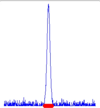
consist of sharp spikes but rather wide-spread Gaussian shaped peaks. Hence, if the algorithm finds a significant feature position, say at the maximum of some peak, it usually tends to select also those features which are close to this position. Such a behavior is not very surprising, because nearby features are highly correlated to the maxi-mum of the peak, and therefore, they may allow for a good separation as well.
Empirical results have shown that this process of selec-tion “evolves” in a continuous fashion when changing the sparsity levelλ. As a consequence, the support of a fea-ture vectorωˆ from Algorithm 2 typically consists of a few connected “intervals” (consecutive sequences of indices) which are centered around the selected peaks (see also Fig. 3). The actual sparsity ofωˆ should be therefore mea-sured by means of its connected intervals and not by simply counting its non-zero entries.
For this reason, we may easily improve the sparsity ofωˆ by reducing every interval to its most significant entry:13 Algorithm 3(Sparsification ofωˆ).
Input:(Sparse) feature vectorωˆ =(ωˆ1,. . .,ωˆd)∈Rd
Output:Sparsified versionω˜ =(ω˜1,. . .,ω˜d)∈Rd
Compute:
1: Find the connected components
A1,. . .,AN ⊂supp(ω)ˆ ofωˆ.
2: For everyl=1,. . .,Ndo the following: Set all entries ofωˆinAlto 0, except from
arg maxk∈A
l| ˆωk|.
Fig. 3Theredstripe indicates the support ofωˆ. Relevant features usually occur as intervals and not as isolated points
3: The resulting vector isω˜.
Step 6: dimension reduction
This final (optional) step does not involve any further computations but shows how to proceed with our resultω˜. As mentioned before, the main purpose of SPA is not just to classify (unknown) samples, but rather to reduce the data to its significant entries (dimensions). Indeed, we may useω˜for adimension reduction: Letx=(x1,. . .,xd)∈Rd
be some (possibly unknown) data vector. Then, we can projectxonto the selected feature positions of supp(ω)˜ . More precisely, all entries that do not belong to supp(ω)˜ are set to 0: ˆ xk := xk, k∈supp(ω)˜ , 0, otherwise, k=1,. . .,d. (12) The resulting data vector xˆ = (xˆ1,. . .,xˆd) ∈ Rd
is now trivially embedded into a low-dimensional space of dimension #supp(ω)˜ .14 But it still contains the most important information which has been found by the above algorithm. Note that we have not made any use of the actual values ofω˜but merely of its support.
By this projection, we may reduce the danger of overfit-ting. In particular, by working in a low-dimensional space, a large tool set frommachine learningis now available for classification and clustering. But how to explicitly proceed with the data heavily depends on the specific application and is therefore not part of SPA.
Results and discussion
Feature selection from simulated data-sets
In this section, we assess our framework of SPA with regard to a typical situation in mass-spectrometry analy-sis: We would like to extract discriminating features from MS data with respect to two groups (e.g., healthy and diseased patients). A major difficulty is usually that only a small number of measurements (observations) is avail-able. Building on this, we ask for the following: Given a simulated data-set for which the position and number of discriminating peaks are known (this will be called ω0 below), how many samples are needed to identify these features with high accuracy?
We shall compare our results to the widely used state-of-the-art algorithms LIBLINEAR (1-regularized SVM) and the standard MATLAB implementation of Lasso.
Creating a simulated data-set
We assume that our sample set{(xi,yi)}i=1,...,n ⊂ Rd× {−1,+1} follows a certain joint random distribution (X,Y), where each sample is independently drawn. In order to make the problem tractable, let us make two model assumptions onXandY. First, the mass spectraX are generated as follows:
xi= M
m=1
smi am+ni, i=1,. . .,n,
where smi ∈Rd determines the (random) amplitude of them-th peak,am∈Rdspecifies its position and shape, andni ∈ Rrepresents the low-amplitude baseline noise.
We shall assume that the amplitudes and the noise are Gaussian, that is, si := (s1i, ...,sMi ) ∼ N(0, ) with
∈ RM×M positive definite and n
i ∼ N(0,σ2I) with
σ > 0. Note that the generated data might have
nega-tive components. This does not mimic the structure of real-world mass spectra which is always non-negative. However, since centering is part of our preprocessing anyway (cf. Step 3 in “Algorithmic details” subsection), the assumption of mean-zero amplitudes is quite natural. The (disease) labels Y are then simply modeled as 1-bit observations (see also (8))
yi=sign(xi,ω0), i=1,. . .,n, (13)
whereω0 ∈Rdis the sparse ground-truth feature vector, which we intend to estimate. In the following, each non-zero entry ofω0is located at the center of a specific peak (see Fig. 4(d)–(f )), so that supp(ω0)actually determines all biologically relevant peaks (molecular structures). Since is invertible (i.e., the features are linearly indepen-dent), this collection of peaks is an optimal fingerprint in the sense that removing or adding any feature variable would decrease the prediction accuracy (with respect to the “perfect” model of (13)).
In our experiments, we create data-sets x1,. . .,xn ∈
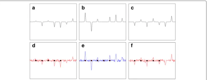
R8192, each one consisting of 200 equidistant peaks (atoms am) shaped like Gaussian density function of width 10. The vector ω0 ∈ R8192 is chosen to have five non-zero components, which means that only five prechosen peaks were used to generate the labelsy1,. . .,yn. Hereafter, we
will refer to these as condition positive peaks. Figure 4 shows three different data instances magnifying only the first seven peaks, generated in the described way. In order to verify our method, we will use two types of data-sets DS1 and DS2 which only differ in their correlation matrix . For DS1, is chosen to be the identity matrix. This implies that the heights of all of the 200 peaks are stan-dard Gaussian random variables. For DS2, we have chosen three pairs of negative peaks to be positively correlated and in addition, one condition positive peak was chosen to be positively correlated with one of the negative peaks. Thus, there are a few entries of value 0.8 off the main diag-onal in . To test the algorithm’s performance increasing amount of Gaussian noise ni ∼ N(0,σ2) with σ = {0.1, 0.3}was added to DS1 and DS2. These corresponds to signal-to-noise (SNR) ratio of 10, 3.33 repectively 15. The values of SNR are chosen to represent the behaviour of the algorithm up to the levels of noise that are normally found in MS data.
Setup and evaluation criteria
Let us recall the essential question of our experiments: Can we recover the support ofω0, and if so, how many samples do we need for that? For this purpose, we shall successively increase the number of available samples in the (training) data-set and examine whether SPA (or
Fig. 4Illustration of the generated data instances.a–c: First seven equidistant Gaussian peaks that are located in fixed positions in each of the three data instances;d–f: Visualization of the data instances from (a)–(c) with additive noise with standard deviationσ =0.1, where the positions of the five condition positive peaks are highlighted byblack dots. Theblueandred colorsindicate the different classes which are determined by the observation process of (13)
Lasso, or1-SVM) succeeds in recovering supp(ω0). Since each of the considered algorithms involves a variable parameter, we have decided to perform an adaptive tuning for each problem instance. In fact, the sparsity parame-ter was chosen such that the resulting classifierω˜matches the sparsity level ofω0. But of course, this does not auto-matically imply that the supports ofω˜ andω0completely coincide.16For each problem instance, the smallest spar-sity parameter which resulted in a classifier with five non-zero entries was chosen in the following way: The ini-tial value of the sparsity parameter for SPA and1-SVM (Lasso) was set to the value which corresponds to the clas-sifier with less than (more than) five non-zero values17. For SPA and1-SVM (Lasso), the sparsity parameter was increased for a preset step size until the outcome had five or more (five or fewer) non-zero entries. If the pre-vious step provided a sparse classifier with strictly more than (strictly less than) five non-zero entries, the bisec-tion method was used on the interval between the two last sparsity parameter values. The bisection method was used until the optimal sparsity parameter was found or the dif-ference between the two consecutive parameters became smaller than a preset tolerance.
We will use a measure based onsensitivity. Sensitivity, defined as18
sens := TPTP+FN
is an appropriate measure for our objectives because it represents an algorithm’s ability to detect the relevant features. Note that ideally, the number of condition posi-tives (TP+FN) is equal to predicted condition positives (TP + FP). In such a situation, the precision, given by p:=TP/(TP+FP)is equal to the sensitivity. However, in the presence of noise it is possible that the final selection encompasses several features which are associated with a single peak. This could lead to a precision value equal to 1 if all of the selected values are declared as true positives, though some other true features remain undetected. Since for us, it is equally important to penalize both false pos-itives and false negatives, we have chosen the sensitivity to be the main point of reference. A measure of similar importance is thespecificity, which is defined by
spec := TN FP+TN.
Finally, due to the possibly imbalanced number of rele-vant features, we shall also take into account the so-called balanced accuracy
bacc := sens+spec
2 .
Results for the simulated data-sets
Data-sets of sample sizes between 50 and 350 were gen-erated as described above and each of the methods was
performed for standardized input data. Note that the hard thresholding step described in (11) was also applied to the classifiers obtained from Lasso or1-SVM. Otherwise, any computational inaccuracy would completely destroy the sparsity structure of the results.
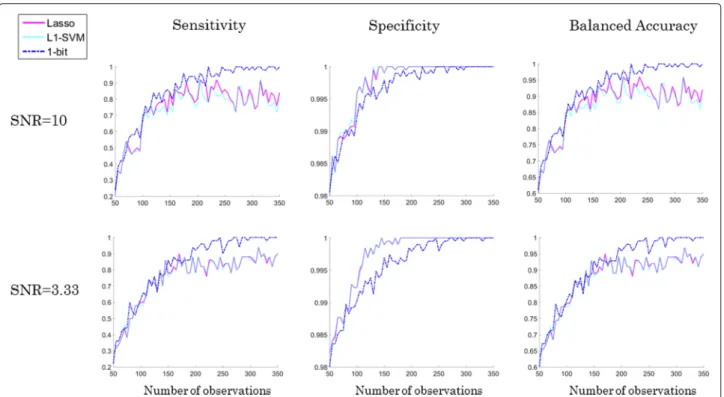
For the sake of statistical stability, each experiment was repeated 10-times. The averaged results are presented in the Fig. 5. We can see that SPA (= 1-bit CS) performs better than the1-SVM or Lasso with regard to the capa-bility of recognizing the true positive features (sensitivity in Fig. 5). In our setting, if one method fails to select 5 condition positive peaks because one of them was selected twice, and the other method selects exactly the same 4 peaks and one false positive in addition, the specificity penalizes only the latter one. But effectively, both cases are suboptimal, since only the 5 positive peaks together can predict the class correctly. This effect is reflected by a smaller value of specificity of the 1-bit approach compar-ing to the specificity of other two methods for data-sets with less than 300 spectra (column 2 in Fig. 5). How-ever, this also implies that SPA performs sligtly worse in rejecting true negatives than the other two approaches. The average results for balanced accuracy are visualized in the third column of Fig. 5. We observe that SPA out-performs the other two methods and even achieves 100% accuracy with relatively few observations. With further decreasing SNR the performance of the three algorithms becomes more similar. Figure 6 shows the numerical out-comes for the data-set DS2. The non-trivial correlation structure of DS2 eventually leads to a slight drop of sen-sitivity and accuracy for SPA (compared to DS1), whereas the performance of the other two methods essentially remains unaffected. As before with further decreasing SNR the performance of the three algorithms becomes more similar in terms of sensitivity and balanced accuracy.
Results for real-world MALDI-TOF MS data
In this section, we present results of SPA, Lasso, and 1-SVM for analyzing real-world mass-spectrometry data and compare them to the MALDIquant proteomics anal-ysis workflow [36]. All data was acquired in our earlier studies [10, 37]. It was approved by the local ethics com-mittees and fulfils the requirements of the Helsinki decla-ration. All subjects gave informed consent to participate in the study. We will demonstrate the performance of our method on two data-sets:
• Spiked data: The spiked data-set is a labelled ground-truth data-set containingcontrol (e.g. healthy) and case (e.g. diseased) mass spectra where the true labels are known. It is created from human blood samples19 which were either unchanged (control group) or in which a protein-mix has been mixed (spiked) into (case group). In order to simulate different strength
Fig. 5Comparison of numerical results for SPA (=1-bit CS), Lasso, and1-SVM on the data-set DS1 with SNR = 10, and 3.33, showed in the
respective row. Note that the data consist of 5 condition positive and 195 condition negative peaks which are equidistantly located in the spectra
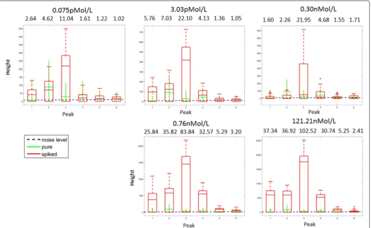
of an effect caused e.g. by a disease, we further sub-divided thecase group into five sub-groups where the amount of spiked-in proteins is increasing. The five volumes in the case sub-groups were spiked with the following concentrations of the protein mix20: 0.075pMol/L, 3.03pMol/L, 0.30nMol/L, 0.76nMol/L and 121.21nMol/L. This mix contains the hormones Angiotensin, ACTH, clip 18-39, Substance P and the cell protein Ubiquitin. The peptide mix was added before sample pre-treatment and 64 spectra were measured due to 4-fold spotting (technical replicates). Mass spectra were acquired using the protocol described in the Additional file 1. Each volume corresponds to a data-set. What differentiates the data-sets are the amplitudes of the 6 spikes resulting from the added substances. The signal-to-noise ratio of the spiked-in peaks is shown in the Fig. 721.
• Pancreas Cancer Data (P. CA) : A total of 120 patients with pancreatic cancer and controls were recruited for this study [10]. For the discovery study sera were obtained from two different clinical centres
(University Hospital Leipzig (UHL, set L) and Heidelberg (UHH, set H)) as described in the
supplementary material (S1). Note that each acquired spectrum has been assigned a class-label, i.e., healthy or diseased. So, the health status of the training samples is known in advance (supervised learning).
Baseline removal was performed on the raw MS data using TopHat filtering ([38]). In particular, no additional calibration or noise reduction steps have been applied. More information on the data and sample preparation can be found in the supplementary material (S1).
The missing-data problem
When dealing with data coming from measurements of, say, a Mass Spectrometer instrument, the so called missing-data problemusually occurs. This means that the instrument failed to give measurements for some of the measured masses, usually due to the stochastic nature of the process happening inside the device. Due to the smoothing step in our algorithm and the arguments of e.g. Rubin et al. ([39]) this problem can be mainly ignored in our case for identifying the relevant features. How-ever, this does not necessarily hold for the classification step, i.e. applying the identified sparse classifier to an unknown data-set. In this scenario, where data is missing
Fig. 7The height of true signals (6 spiked in peaks) comparing to the height of noise and height of the corresponding values in the pure data-set. Signal-to-noise ratio, which was calculated as the ratio of median of spiked-in signals and the estimated level of noise is shown above the corresponding peaks
in an unknown sample, there are basically two options: (1) applying a method for inferring the missing data or (2) stopping the classification and return an error message to the user. In this work we decided to follow the latter approach, since inferring missing data is not in the scope of this paper22 but is an unarguable crucial point in any data analysis pipeline and should depend on the actual use-case.
Accuracy vs. number of features
We performed thereal worldexperiments with respect to the same evaluation categories as in the case of simulated data. Note that the normalization and standardization as described in “Algorithmic details” section were applied as preprocessing steps in each of the methods. Similarly, a hard thresholding as described in (11) was applied to all classifiers estimated by the examined algorithms.
For the each of the algorithms, we are testing the per-formance of the obtained classifiers learned on the pure data-set which corresponds to the condition negative class and one spiked data-set at a time corresponding to the condition positive class.
The results of the classifier with 6 non-zeros on the spiked data-set are shown in Table 2. The main ques-tion in these experiments is how successful each of the algorithms is in detecting the 6 peaks that were initially spiked (see the data-set description above). We can see that the values of sensitivity for SPA are at least as high as those of the other methods, which implies that the approach of 1-bit CS is very competitive in this situation and mostly achieves the best detection rate. However, the relatively poor performance of all the algorithms on the spiked data-set can be explained by the nature of the data. Since the peptide mix was added to the blood samples before acquiring the mass spectra, the spiked peaks are not always present in all the resulting mass spectra in the positions where we expect to find them. There exist data-sets for which all the mass spectra failed to exhibit certain spiked peaks at their expected locations. as can be seen in the Fig. 7. Thus, we cannot expect any of the algorithms
to find these missing peaks. Nonetheless, there is still a chance to build a reliable fingerprint out of the remain-ing spikes while there is no chance to detect the missremain-ing spikes because the data-set is not rich enough to represent it. On the other hand, this spiked data-set combines the advantages of both simulated and clinical data, since the positions of the desired biomarkers are known in advance while their representative behavior in the spectra is quite realistic.
In contrast to that in the case of pancreas cancer data-sets, we do not know the true-positive feature posi-tions. Consequently, we can only rely on the classifica-tion performance of the obtained sparse classifiers by each of the algorithms. To evaluate the reliability of our results, for each of the methods, we have employed the cross-validation scheme as described in the Algorithm 4 with the number of folds K set to 5. In order to ensure statistical stability, each experiment was repeated 10-times. Figure 8 shows the average results over 10 repetitions.
Algorithm 4 (Cross-Validation of Classification Perfor-mance).
Input: Raw data (x1,y1),. . .,(xn,yn) ∈ Rd × {−1,+1};
Number of CV-foldsK;
Output: Classification accuracy Acc ∈ [0, 1]; Average sparsity #F(number of selected features)
Compute:
1: Split the sample set{1,. . .,n}randomly intoK disjoint foldsP1,. . .,PK of (almost) equal size.
For each foldk∈1,. . .,Kperform the following steps 2-4:
2: Compute the feature vectorωkemploying the desired method on the samples ofk∈{1,...,K}\{k}Pk
3: Dimension reduction as described in Algorithmic Details (step 6). Project all spectra onto supp(ωk)and put#Fk := ||ωk||0.
4: Classification of Pk: Use the projected samples of k∈{1,...,K}\{k}Pkto predict the labels of the spectra
Table 2This table shows the main results comparing the feature selection benchmarks of our approach with Lasso and1-SVM on the
spiked data-set. Given results correspond to the average results over 10 repetitions of the classifier with 6 non-zero values
SPA Lasso 1-SVM
Concentration TP[a] Sens[b] Specs[c] B. Acc[d] TP Sens Spec B. Acc TP Sens Spec B. Acc
0.075pMol/L 2 0.333 1.000 0.667 1 0.167 1.000 0.583 1 0.167 1.000 0.583
3.03pMol/L 4 0.667 1.000 0.833 2 0.333 1.000 0.667 1 0.167 1.000 0.583
0.30nMol/L 2 0.333 1.000 0.667 1 0.167 1.000 0.583 1 0.167 1.000 0.583
0.76nMol/L 2 0.333 1.000 0.667 2 0.333 1.000 0.667 2 0.333 1.000 0.667
121.21nMol/L 3 0.500 1.000 0.750 2 0.333 1.000 0.667 2 0.333 1.000 0.667
[a]TP: Number of spiked peaks that are correctly detected [b]Sens: Sensitivity in detecting spiked peaks (TP/(TP+FN)) [c]Spec: Specificity in detecting spiked peaks (TN/(FP+TN)) [d]B. Acc: Balanced Accuracy (sens.+spec.
Fig. 8Accuracies of sparse classifiers from SPA, Lasso, and1-SVM on the real pancreatic cancer data-sets. While Lasso and1-SVM achieve better
classification accuracy with increasing number of features, SPA is particularly well suited for the “very-sparse regime” where only few features (<20) are used for classification
Pkby an ordinary SVM[1]. Denote the prediction
accuracy byAcck.
5: Compute the average accuracyAcc := K1 Kk=1Acck
and average sparsity#F:= K1Kk=1#Fk.
In order to ensure statistical stability, each experiment was repeated 10-times. Figure 8 shows the results. Note that our results show that accurate predictions are already possible with a very few features, so that the assump-tion of small disease fingerprint seems to hold for this data-set. Furthermore, it can be seen that SPA is espe-cially well suited for situations where a sparse classifier (containing only very few features) is preferred. This is appealing because fewer features enable an easier inter-pretation of the actual components of a potential disease fingerprint. Moreover, follow-up experiments that often involve an individual treatment of each component (e.g., potential biomarkers) would become much less costly. Note that in the non-sparse region with more than 30 fea-tures selected, it is not meaningful to relate the achieved accuracy to the quality of the learned feature vector due to the small sample size. The considered algorithms assume the underlying fingerprint to be sparse. This assumption usually does not fully hold in practice. Therefore, we can-not expect that a learned feature vector achieves perfect classification. The classification accuracy should be there-fore considered as an indicator of how well our model assumption of the sparse fingerprint fits to the unknown ground-truth. If we let the algorithms operate out of the region for which they have been designed for, we may achieve indeed a higher accuracy, but this is probably a consequence of overfitting. And even more importantly,
the learned feature vector (model) is not reliable any-more.23
Best classifier
Apart from that, we are interested in the performance of the best sparse classifier (i.e. small number of features) found by each of the algorithms (SPA, Lasso,1-SVM). For all learned classifiers with 10 to 30 non-zero com-ponents, Table 3 presents those with the best classifica-tion accuracy. Furthermore, we also considered a typical analysis pipeline (MALDIQuant) to see how the “purely-data-based” approaches (SPA, Lasso, 1-SVM) compare to a model-based approach24. In Table 3, it can be seen that SPA provides the sparsest solutions while achieving competitive results with respect to sensitivity and speci-ficity at the same time. Lasso and1-SVM select almost the same features and therefore perform similarly. On the other hand, MALDIQuant selects the features based on a prior model-based peak detection followed by a fea-ture selection based on shrinkage diagonal discriminant analysis ([40]). But however, it still performs worst on the UHL data-set.
Medical interpretation of results
Pancreatic cancer is not only a common and increasingly frequent [41], but also still a fatal disease, with a survival rate of 3-5% five years after diagnosis [42]. The conventional tumor marker, Carbohydrate Antigen 19-9 (CA19-9), as a blood group antigen not present in a significant proportion of the patients [43], shows insufficient diagnostic sensitivity and specificity (AUC 0.71), even in combination with the second-line tumor marker Carcinoembryonic Antigen (CEA, combined
Table 3 This table shows the main results comparing the feature selection benchmarks of our approach with Lasso, 1 -SVM, and Maldi-Quant. These are averages over 10 repetitions of a 5-fold cross-validation. Note that these results have been calculated based on the highest accuracy criterion for all classifiers with between 1 0 and 30 selected features. This particularly means that better accuracy values might be achieved for the individual methods if less sparse feature vectors would be allowed. For more details see text SPA Lasso 1 -SVM Maldi-Quant Dataset Feat. [ e ] Sens [ f ] Spec [ g ] B. Acc [ h ] Feat. Sens Spec B .Acc Feat. Sens Spec B .Acc Feat Sens Spec B. Acc P. CA -U HL 20.48 0.975 0.949 0.962 29.94 0.969 0.939 0.954 27.72 0.964 0.947 0.955 21 0.888 0.888 0.888 P. CA -U Hh 17.1 0.986 0.975 0.981 26.46 0.966 0.969 0.967 29.68 0.966 0.976 0.971 17 0.975 0.963 0.969 [ e ]Feat.: Number of features [ f ]Sens: Sensitivity ( TP /( TP + FN ) ) [ g ]Spec: Specificity ( TN /( FP + TN ) ) [ h ]B. Acc: Balanced A ccuracy ( sens. + spec. 2 )
AUC 0.75) [44]. The need for better markers for screen-ing and differential diagnosis is evident, as panceratic carcinoma would be principally curable if detected and identified very early in the course of the disease. Along with the emerging “-omics”-technologies great hope was rised to find tumor-specific peptides or metabolic alterations to increase sensitivity and specificity of early and differential diagnostics, and several combinatory marker models could be identified by proteomics [10] and metabolomics [45]. Pancreatic carcinoma is a complex disease - it affects the metabolism as a whole (e.g. the so-called Warburg effect) [46], but also alters proteolytic activity [47]. Therefore, it might be naïve to expect a single marker capable to indicate presence, progression and exact type of the malignancy at once [48] 9– it might even be overly reductionistic to attribute these capabilities to a single model, even if it consists of several entities measured by different “- omics” technologies [43]. As Raftery states “basing inferences on a single “best” model as if the single selected model were true ignores model uncertainty, which can result in under-estimating uncertainty about quantities of interest” [49], and the larger the “-omics” data-sets grow, the larger is the ‘probability, that there is not one “single best” predictive marker model, but instead several with comparable selectivity [48]. And it is very reasonable to assume that, even on the same data-set, different algorithms might favor different models consisting of different feature sets and bring forth completely different results, when only the best differentiating models are regarded. For an in-depth comparison of the validity of the results of different algorithms, the underlying peak features should also be taken into account, and similar-ities in the selected features corroborate the algorithms superimposed on them. In the case of our study, we have the great advantage, that the same data-set was evaluated in three different studies: the principal one by Fiedler et al. [10], a subsequent BinDA-algorithm-based manuscript by Gibb and Strimmer published recently [50], and the present one. Fiedler et al. [10] identified one discriminating peptide, Platelet Factor 4 (m/z3884, identified in italics, double hits in bold) within four discriminating peaks (m/z 3194,3884, 4055, and 5959). The 30 most differential peaks in Gibb et al. [50] were m/z 4495, 8868, 8989, 1855, 4468, 8937, 2023, 1866, 5864, 5946, 1780, 2093, 5906, 5960, 8131, 1207, 4236, 2953, 9181, 1021, 1466, 4092, 4251, 5005, 8184, 1897, 3264, 2756, 6051, and 1264, with m/z 8937 identified as pan-creatic progenitor cell differentiation and proliferation factor-like protein. m/z 3884 could not be identified as discriminating marker (while it might play a role in pancreatic carcinoma nonetheless [51]), whereas m/z
1466can be attributed to a fragment of fibrinopeptide A (DSGEGDFLAEGGGVR), as previously described in
tumor samples [52]. In the present study, the peaks m/z
1464, 1546, 1944, 5904, 1619, 4209, and 2662 could be identified as discriminating features. The slight mass shift of about 2 Da for m/z1464/1466and5904/5906 is probably arising from different peak preprocessing procedures, peaks are wide enough to tolerate this deviation. Further investigations and the application of further algorithms on the same data-set are highly likely to yield a similar, partially overlapping set of features, each with a comparable discriminating power (Fiedler et al. [53] AUC[3884/(CA19−9∗CEA)]1.0; Gibb et al. [50] in a 5-feature model: accuracy of 0.96, sensitivity of 0.96, specificity of 0.97, positive predictive value of 0.97 and negative predictive value of 0.95; the present study accuracy[UHL] 0.96, sensitivity[UHL] 0.97, specificity[UHL] 0.95 and accuracy[UHH] 0.98, sensitivity[UHH] 0.99, specificity[UHH]0.97. This also corresponds to a recently published comparable study investigating a glycoprotein marker panel (AUC 0.95) [54]. Biomarkers for clinical diagnostics comprise a wide field of applications (e.g. population-wide screening, early diagnostics, charac-terization, treatment guidance, efficacy and toxicity monitoring, prognosis, susceptibility estimation and many more) [43], each with special requirements for sensitivity and specificity, that are only partially con-densed in the AUC as an overall selectivity measure [48]. Especially for screening purposes, sensitivity is extremely important [45], and clinically applied tests e.g. for new-born screening frequently surpass the 0.99 hallmark [53]. Compared with the conventional, “not-for-screening” marker CA19-9, the SPA-based model shows consid-erable improvement, however there is still a big gap to screening suitability, which in the next years might be bridged by improved sensitivity of new instrumentation, refined algorithms (as the SPA), and combination with other “markers” from the “big data” field, enabling a more holistic view – not only of the disease, but also of the affected patient [43].
Conclusions
Workflows for analyzing high-dimensional (bio-medical) data often contain a step where discriminating fea-tures between two groups need to be identified. This is important for applications such as classification and clustering but is also essential for understanding bio-logical differences, e.g. between two phenotypes. In this paper we have presented a new algorithm based on the theory of Compressed Sensing that identifies the minimal set of such features. This is of par-ticular importance for modern, very high-dimensional data-sets such as proteomics mass-spectrometry data to allow interpretation of the results. Our experiments and comparisons to state-of-the-art algorithms show that our method finds smaller features sets resulting in