LUO, BIN, Ph.D. Robust Penalized Regression for Complex High-dimensional Data. (2020)
Directed by Dr. Xiaoli Gao. 169 pp.
Robust high-dimensional data analysis has become an important and chal-lenging task in complex Big Data analysis due to the high-dimensionality and data contamination. One of the most popular procedures is the robust penalized regression. In this dissertation, we address three typical robust ultra-high dimensional regression problems via penalized regression approaches. The first problem is related to the linear model with the existence of outliers, dealing with the outlier detection, variable selection and parameter estimation simultaneously. The second problem is related to robust high-dimensional mean regression with irregular settings such as the data contamination, data asymmetry and heteroscedasticity. The third problem is related to robust bi-level variable selection for the linear regression model with grouping structures in covariates.
In Chapter 1, we introduce the background and challenges by overviews of penalized least squares methods and robust regression techniques. In Chapter 2, we propose a novel approach in a penalized weighted least squares framework to perform simultaneous variable selection and outlier detection. We provide a unified link between the proposed framework and a robust M-estimation in general settings. We also establish the non-asymptotic oracle inequalities for the joint estimation of both the regression coefficients and weight vectors. In Chapter 3, we establish a framework of robust estimators in high-dimensional regression models using Penalized Robust Approximated quadratic M estimation (PRAM). This framework allows general settings such as random errors lack of symmetry and homogeneity, or covariates are not sub-Gaussian. Theoretically, we show that, in the ultra-high dimension setting,
the PRAM estimator has local estimation consistency at the minimax rate enjoyed by the LS-Lasso and owns the local oracle property, under certain mild conditions. In Chapter 4, we extend the study in Chapter 3 to robust high-dimensional data analysis with structured sparsity. In particular, we propose a framework of high-dimensional M-estimators for bi-level variable selection. This framework encourages bi-level sparsity through a computationally efficient two-stage procedure. It produces strong robust parameter estimators if some nonconvex redescending loss functions are applied. In theory, we provide sufficient conditions under which our proposed two-stage penalized M-estimator possesses simultaneous local estimation consistency and the bi-level variable selection consistency, if a certain nonconvex penalty function is used at the group level. The performances of the proposed estimators are demonstrated in both simulation studies and real examples. In Chapter 5, we provide some discussions and future work.
ROBUST PENALIZED REGRESSION FOR COMPLEX HIGH-DIMENSIONAL DATA
by Bin Luo
A Dissertation Submitted to the Faculty of The Graduate School at The University of North Carolina at Greensboro
in Partial Fulfillment
of the Requirements for the Degree Doctor of Philosophy
Greensboro 2020
Approved by
APPROVAL PAGE
This dissertation written by Bin Luo has been approved by the following committee of the Faculty of The Graduate School at The University of North Carolina at Greensboro. Committee Chair Xiaoli Gao Committee Members Sat Gupta Quefeng Li Scott Richter Haimeng Zhang
Date of Acceptance by Committee
ACKNOWLEDGMENTS
Foremost, I wish to express my deep gratitude to my advisor Dr. Xiaoli Gao for her strong support and insightful guidance throughout my Ph.D. study and research, for her patience, enthusiasm and continuous encouragement. Without her persistent help, I would not have achieved what I have now.
I would also like to thank Dr.s Sat Gupta, Quefeng Li, Scott Richter and Haimeng Zhang for their service on my committee. I really appreciate the precious learning opportunity and environment provided by the Department of Mathematics and Statistics at UNC Greensboro.
I am very grateful to my family, who are always doing their best to support me throughout my life.
Lastly, I would like to thank my wife, Yang, for being extremely supportive and making countless sacrifices to help me get to this point.
TABLE OF CONTENTS
Page
LIST OF TABLES. . . vi
LIST OF FIGURES. . . vii
CHAPTER I. INTRODUCTION . . . 1
I.1. Background and Challenges . . . 1
I.2. Penalized Least Squares Method . . . 5
I.3. Robust Penalized Regression Method . . . 15
I.4. Main Contributions . . . 27
II. PENALIZED WEIGHTED LEAST SQUARES METHOD . . . 32
II.1. Introduction . . . 32
II.2. Weight Shrinkage . . . 33
II.3. Implementation. . . 37
II.4. Non-asymptotic Properties . . . 40
II.5. Numerical Result . . . 44
III. PENALIZED ROBUST APPROXIMATED QUADRATIC M-ESTIMATORS. . . 55
III.1. Introduction . . . 55
III.2. The PRAM Method . . . 58
III.3. Statistical Properties . . . 64
III.4. Implementation of the PRAM Estimators . . . 72
III.5. Simulation Studies . . . 73
IV. HIGH-DIMENSIONAL M-ESTIMATION FOR BI-LEVEL
VARI-ABLE SELECTION . . . 82
IV.1. Introduction . . . 82
IV.2. The Two-stage M-estimator Framework . . . 84
IV.3. Statistical Properties . . . 89
IV.4. Implementation. . . 95
IV.5. Simulation Studies . . . 96
IV.6. Real Data Example . . . 103
V. DISCUSSION AND FUTURE WORK . . . 106
V.1. On the Penalized Weighted Least Squares Method . . . 106
V.2. On the Penalized Robust Approximated Quadratic M-estimators . . . 108
V.3. On the High-dimensionalM-estimation for Bi-level Vari-able Selection . . . 110
BIBLIOGRAPHY . . . 112
LIST OF TABLES
Page
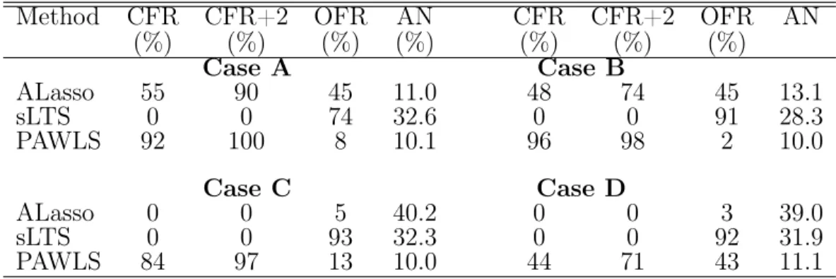
Table II.1. Variable Selection Results for Example II.1 . . . 48
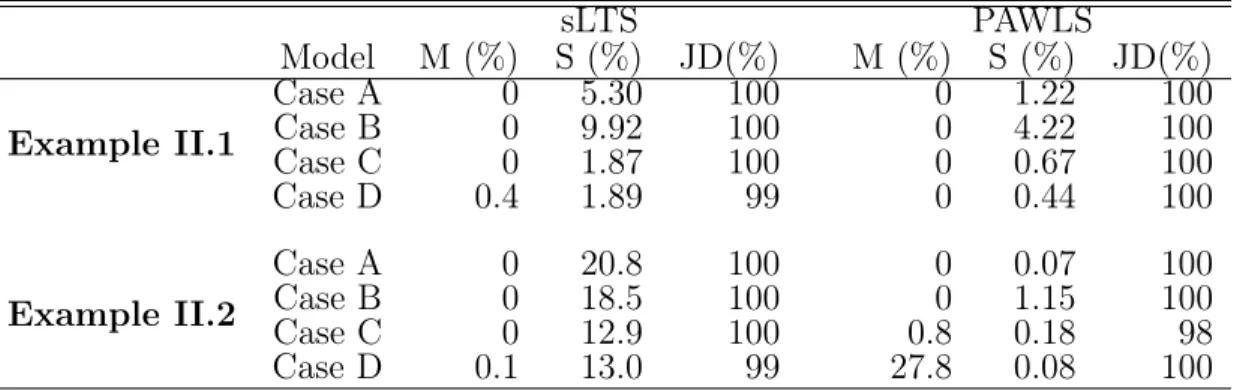
Table II.2. Outlier Detection Evaluation in Example II.1 and II.2 . . . 48
Table II.3. Variable Selection Results for Example II.2 . . . 50
Table II.4. Estimation Regression Coefficients from Air Pollution Dataset . . . 52
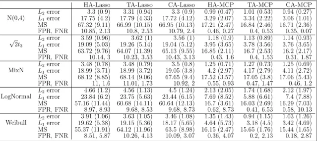
Table III.1. Simulation Results under the Homogeneous Model with Standard Normal Covariates in Example III.1 . . . 77
Table III.2. Simulation Results under the Heteroscedastic Model with Standard Normal Covariates in Example III.2 . . . 77
Table III.3. Simulation Results under the Homogeneous Model with Non-Gaussian Covariates in Example III.3 . . . 78
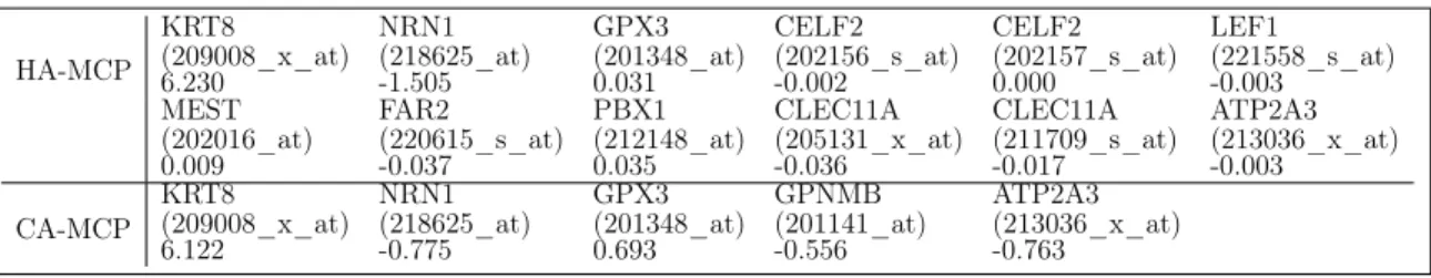
Table III.4. Selected Genes and the Corresponding Coefficient Estimation by HA-MCP and CA-MCP . . . 79
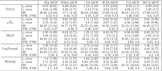
Table IV.1. Simulation Results under the Model with Only Between-group Sparsity in Example IV.1 . . . 100
Table IV.2. Simulation Results under the Model with Bi-level Sparsity in Example IV.2.1 . . . 101
Table IV.3. Simulation Results under the Model with 20% Contamination on X in Example IV.3. . . 102
Table IV.4. Selected Genes by Huber-MCP, Cauchy-MCP, Huber-GMCP, Cauchy-GMCP, Huber-GMCP-HT, Cauchy-GMCP-HT . . . 104
LIST OF FIGURES
Page
Figure II.1. Display of Some Functions . . . 36
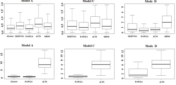
Figure II.2. Boxplot of MSE in Example II.1 . . . 49
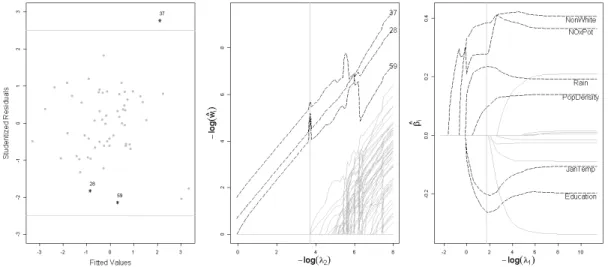
Figure II.3. Air Pollution Data Analysis. . . 52
Figure II.4. NCI-60 Data Analysis . . . 53
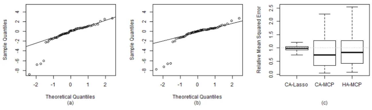
Figure III.1. (a) The QQ Plot of the Residuals from HA-MCP. . . 80
Figure IV.1. QQ Plots of the Residuals from Huber-MCP, Cauchy-MCP, Huber-GMCP, GMCP, Huber-GMCP-HT, Cauchy-GMCP-HT. . . 105
CHAPTER I INTRODUCTION I.1. Background and Challenges
Due to the rapid development of advanced technologies over the last decades, high-dimensional data arise in many scientific fields, with the trend towards radically larger numbers of variables (p) but relatively small number of observations (n), i.e. p n. For example, in biomedical studies, huge numbers of magnetic resonance images (MRI) and functional MRI data are collected for each subject with hundreds of subjects involved. Satellite imagery has been used in natural resource discovery and agriculture, collecting thousands of high resolution images. These kind of examples are plentiful among fields of science, engineering and humanities and new knowledge need to be discovered by using these massive high-throughput data [D+00, FL06].
The high-dimensionality of data has posted some challenges in data analysis. One of them is the intensive computation inherent in these high-dimensional mathemat-ical problems. Systematmathemat-ically searching through a high-dimensional space is usually computational infeasible. At the same time, high-dimensionality has significantly challenged traditional statistical theory. For instance, in term of asymptotic theory, the traditional approximation assumes that n→ ∞ whilep remain smaller order than n or usually fixed. However, the high-dimensional scenario would imagine that p goes to infinity faster than n [JT09]. Other challenges incurred by high-dimensionality also include how to efficiently estimate model parameters in high-dimensional spaces and how to obtain an interpretable model with a large number of variables.
In recent decades, a great number of statistical methods, algorithms and theories have been developed to perform high-dimensional data analysis (HDDA). Among them, penalized least squares (PLS) methods have become very popular in high-dimensional linear regression analysis since the introduction of the LASSO [Tib96a]. A PLS approach is to minimize the penalized objective function combined with both the `2 loss and a penalty on the coefficients vector. When the penalty is
designed to obtain exactly zeros for some coefficients, and nonzero for others, the PLS can perform a simultaneous coefficient estimation and variable selection process, which is attractive in HDDA.
However, the PLS approach may lose its efficiency in both estimation and variable selection in presence of irregular settings such as data contamination. In fact, high-dimensional data can be complex in general: (a) the data are contaminated in both response and a large number of variables [RL05]; (b)the data are highly skewed and heteroscedastic [ZFB14, FLW17]; (c) the covariates possess complex grouping structures [YL06, HBM12]. Hence more sophisticated methods are needed to deal with the high-dimensional complex data.
I.1.1. Data Contamination
In real applications, the data can be contaminated due to the existence of outliers. An outlier is defined as an observation that is very different from other observations based on certain measure. The presence of outliers can lead to biased estimation of parameters, misspecification of the model and misleading predictions. This phenomenon become even more common and challenging in high-dimensional settings. For example, in gene expression analysis, outliers are often produced due to the complicated data generation process. To perform robust variable selection and parameter estimation in HDDA, extensive work on penalized robust M-estimators
has been investigated, such as Huber-Lasso [H+64, LLZ+11] and LAD-Lasso [GH10, Wan13]. Besides, outliers detection also plays a fundamental role in dealing with data contamination. It has important applications in the field of fraud detection, network robustness analysis and intrusion detection. To detect outliers or influential points in high-dimensional regression model, a few diagnosis measures, such as High-dimension Influence Measure (HIM) [ZLL+13], have been proposed.
I.1.2. Data Asymmetry and Heteroscedasticity
Asymmetry along with heteroscedasticity or contamination often occurs with the growth of data dimensionality. In high-dimensional settings, particularly when random errors follow irregular distributions such as asymmetry and heteroscedasticity, simultaneous mean estimation and variable selection are still of interest in many applications. For example, in economics where asymmetric data is prevalent, it is still of interest to study how mean GDP is affected by many features. Another example can be found in RNA-seq data analysis, the highly skewed nature and mean-variance dependency of RNA-Seq data may pose difficulties on building prognostic gene signatures.
[H+64] implies that the location estimator generated by Huber’s method is
possibly biased for certain fixed asymmetric contamination. For M-estimation in linear regression model, [Car79,CW88] indicate that data asymmetry does not affect the slope estimation asymptotically when the error and covariates distributions are independent. However, the case of asymmetric and heteroscedastic errors was not well addressed. [FLW17] further points out that most of penalized robust M-estimators generate bias to the conditional mean regression function when the error distribution is asymmetric and heteroscedastic. Thus it remains a challenge to effectively reduce the bias generated by asymmetric distribution under data contamination in high-dimensional settings.
I.1.3. Grouping Structure in Covariates
Covariates often function group-wisely in many applications. For example, in gene expression analysis, genes from the same biological pathways may exhibit similar activities. In high-dimensional data analysis, bi-level sparsity is often assumed when covariates function group-wisely and sparsity can appear either at the group level or within certain groups. Penalized least squares approaches with penalties incorporating grouping structures, such as the group Lasso [YL06], have become very popular in recent decades. To avoid the all-in or all-out variable selection at the group level, extensive methods such as the sparse group Lasso [FHT10, SFHT13] have been investigated to perform bi-level variable selection. However, when the data are contaminated or heavy-tailed in high-dimension settings, it remains a challenge to perform robust bi-level variable selection and parameter estimation.
I.1.4. Real Data Example
We close this section by introducing a real data example. The NTC-60 data is a gene expression data set collected from Affymetrix HG-U133A chip, which is corresponding to a high-dimensional case (p > n). The dataset consists of data on 60 human cancer cell lines and can be downloaded via the web application CellMiner (http://discover.nci.nih.gov/cellminer/). The study is to predict the protein expression on the KRT18 antibody from other gene expression levels. The expression levels of the protein keratin18 is known to be persistently expressed in carcinomas [OBC96]. And the response variable is chosen from variables with the largest MAD. After removing the missing data, there aren = 59samples with21,944 genes in the dataset. One can refer [SRN+07] for more details.
[LLLP11] applies only non-robust regression methods to this data and obtains models with hundreds of predictors that are thus difficult to interpret. In this thesis,
considering the possible irregularity in the dataset, the robust high-dimensional data analysis approaches are applied.
I.2. Penalized Least Squares Method
To enhance model interpretability and make statistical inference feasible in high-dimensional regression models, the sparsity condition is proposed that among a large set of variables only a few of them are relevant. In such cases, variable selection techniques are crucial for identifying important variables and improving estimation accuracy. For last decades perhaps the most popular approaches for sparse high-dimensional models are the Penalized Least Squares (PLS) methods. The other techniques include sequential approaches (e.g. LARS [EHJ+04], Forward Regression
[Wan09], Sequential Lasso [LC14]) and screening methods (e.g. Sure Independence Screening [FL08], Sure Independent Ranking and Screening [ZLLZ11], nonparametric independence screening [FFS11]).
Consider a high-dimensional linear regression model
yi =xTiβββ+i, 1≤i≤n, (I.1)
where yi and xi = (xi1,· · · , xip)T are the observed response variable and covariates
vector, 1, . . . , are i.i.d. random variables with mean 0 and variance σ2. Note that
βββ∗ = (β1∗,· · · , βp∗)T ∈
Rp is an s-sparse coefficient vector (only include s nonzero
elements) and pn. A class of PLS estimators forβββ∗ takes the following form
ˆ β β β = argmin β β β∈Rp ( n X i=1 (yi−xTiβββ) 2+ρ λ(βββ) ) , (I.2)
where ρλ is a penalty function and λ is a tuning parameter in the penalty. The form
of ρλ determines the flavor of penalized regression and λ controls the magnitude of
with the ordinary least squares estimator. In most scenarios, the penalty function is coordinate-separable such that
ρλ(βββ) = p
X
j=1
ρλ(βj),
for some scalar functionρλ :R7→R.
The work of AIC [Aka98] and BIC [S+78] suggests to choose a parameterβββ that minimizes the penalized least squares in (I.2) with the `0-norm penalty
ρλ(βββ) = λkβββk0 = p
X
j=1
I(βj 6= 0),
when the random error is normal. With the `0-norm penalty, the PLS method
can be viewed as a model selection approach that penalizes the number of variables in the model. However, this penalized `0 regression is unstable with respect to
small perturbations in the data, since the `0 penalty is not continuous. It is also
computational infeasible in the high-dimensional space.
[FF93] generalizes the penalized `0 regression to the bridge regression by
considering ρλ(βββ) =λ P X j=1 |βj|γ for 0< γ ≤2.
It bridges the penalized `0 regression (γ →0) to the ridge regression [HK70] (γ = 2).
When γ ≤ 1, the component of βββ in (I.2) can be shrunk to zero if λ is sufficiently large, thus achieving simultaneous coefficient estimation and variable selection. While the bridge penalty with γ <1 is continuous, its infinite derivative at the origin may cause numerical problem.
The special case when γ = 1 is related to the least absolute shrinkage and selection operator (Lasso) [Tib96a], which is a very popular shrinkage method for
variable selection. The Lasso penalty (`1 penalty) can be viewed as a convex surrogate
of the`0penalty. But it is more stable due to its continuity and computationally feasible
for high-dimensional data. From the Bayesian perspective, the Lasso estimator can be interpreted as a Bayesian posterior mode estimate when the regression parameters have independent Laplace (i.e., double-exponential) priors [PC08].
The statistical properties of the Lasso estimator have been extensively studied (e.g. [KF00], [EHJ+04], [Zou06], [ZY06], [ZH06], [ZH+08],[MY+09] and [BRT09]).
[FL01] shows that the Lasso shrinkage produces biased estimates for the large coeffi-cient. [BRT09] presents that the Lasso is asymptotically equivalent to the Dantzig selector [CT07], with the `2 error rate of prediction or estimation being s/nlog(p),
where the number of variable p can be much larger than the sample size n. [ZY06] characterizes the model selection consistency of the Lasso by proposing the property of sign consistency, P sgn(βββ∗) =sgn(ˆβββ) →1 asn → ∞,
where sgn(βββ) is a vector of signs of βjs and sgn(0) is defined as 0. They show that
the Lasso is sign consistent if the following irrepresentable condition is satisfied, kXT2X1(XT1X1)−1sgn(βββ1)k∞ <1,
where βββ1 is the subvector of βββ∗ on its support supp(βββ∗), and X1 and X2 are the
submatrices of the n×p design matrixX formed by its columns insupp(βββ∗)and its complement, respectively. However, the irrepsentable condition is easily violated in present of highly correlated variables and therefore very restricted in high dimensions. This explains why the Lasso estimator tend to include many false positive in the selected model [FL10].
[FL01] introduces the oracle property for model selection. LetS ={j :βj∗ 6= 0} be the index set of important variable. We call the PLS method in (I.2) an oracle procedure ifβββˆ satisfies (asymptotically) the following oracle properties:
(1) Consistency of variable selection,{j : ˆβj 6= 0}=S and
(2) Asymptotic normality, √n(ˆβββS−βββ∗S)→dN(0,Σ∗),
where Σ∗ is the covariance matrix knowing the true subset model. [FL01] studies the oracle properties of nonconcave penalized likelihood estimators in the finite-dimensional setting. They propose the Smoothly Clipped Absolute Deviation (SCAD) penalty given as follows: ρλ(t) = λ|t| f or |t| ≤λ, −t2−2(a2aλ−|t1)|+λ2 f or λ <|t| ≤aλ,
(a+1)λ2
2 f or |t|> aλ,
(I.3)
where a >2is a fixed parameter. They show that the local minimum in (I.2) with the SCAD penalty satisfies the oracle properties under some regular conditions. [FP+04]
further extends this result to a high-dimensional setting withp=o(n1/5)orp= o(n1/3).
Due to the concavity of the SCAD penalty, it suffers from the multiple minima issue. [KCO08] later shows that with high probability the oracle estimator βββˆO is actually a local minimum of the PLS with SCAD penalty, allowingpto grow withnexponentially. They also provide sufficient conditions to check when a local minimum becomes a global minimum.
[Zou06] shows that the Lasso estimator does not have the oracle properties in general and proposes the adaptive lasso that uses the weighted `1 penalty,
ρλ(βββ) =λn p
X
j=1
wj|βj|,
where wj = 1/|β˜j|γ andβββ˜ is an root-n consistent estimator ofβββ
∗
which serves as an initial estimator for the adaptive Lasso procedure. Note that for any fixed λ, the penalty for zero-initial estimation goes to infinity, while weights for nonzero initials converge to a finite constant. Consequently, by allowing a relatively higher penalty for zero-coefficients and lower penalty for nonzero coefficients, the adaptive lasso is able to reduce the estimation bias and improve variable selection accuracy. Similar to the Lasso, solving for the adaptive Lasso is also a convex optimization problem and thus it does not have the issue of multiple local minima.
For fixedp, [Zou06] proves that the adaptive LASSO has the oracle property. In high dimension setting, forpn, [HMZ08] shows that under the partial orthogonality and certain other conditions, the adaptive LASSO obtains variable selection consistency and estimation efficiency, when the marginal regression estimators are used as the initial estimators.
[Z+10] proposes the Minimax Concave Penalty (MCP) that shares a similar
spirit as the SCAD penalty. The MCP takes the form ρλ(t) =sign(t)λ Z |t| 0 1− z λb + dz,
with a fixed parameter b >0. It minimizes the maximum concavity κ(ρ) := sup
0<t1<t2
subjects to the following unbiasedness and selection features ρ0λ(t) = 0 for t ≥bλ and ρ0λ(0+) =λ.
It has been proved that the local minima of the PLS in (I.2) with MCP have the oracle properties under some regular conditions. Specially, [Z+10] proposes the Penalized
Linear Unbiased Selection (PLUS) algorithm with MCP to obtain local minimizers that equal the oracle estimatorβββˆO, with the probability converging to 1.
The above motioned folded-concave penalty, i.e. the SCAD penalty and the MCP, can be viewed as interpolations between the `0 penalty and the `1 (Lasso)
penalty. One one hand, the folded-concave penalties possess smoothness over the `0
penalty to gain flexibility and stability in computations. On the other hand, they can reduce the bias of the Lasso and thus improve model selection accuracy and obtain oracle properties. [FL11] investigates the penalized likelihood approaches using a general class of folded-concave penalty functions in the context of generalized liner model. They demonstrates that such methods have oracle properties with the dimensionality of non-polynomial order of the sample size.
Although these methods enjoy many attractive statistical properties, they do not work well when the covariates are highly correlated or have certain grouping structures. For example, in gene expression analysis, genes from the same biological pathways may have strong correlations. [Tib96a] points out that when there are highly correlated predictor in high-dimensional settings, the prediction performance of the Lasso is dominated by the ridge regression. [ZH05] demonstrates that the Lasso tends to select one variable among a group of highly correlated covariates.
To address these issues, [ZH05] proposes to use the elastic net (Enet) penalty, which is the linear combination of the `1 and `2 penalties
ρλ1,λ2(βββ) = λ1kβββk1+λ2kβββk2,
where λ1, λ2 > 0 are the tuning parameters. The Enet penalty can encourage the
sparsity and grouping effects simultaneously. [YL07] and [JY10] investigate its selection consistency in the settings whenpis fixed andpn, respectively. They show that the Enet estimator is selection consistent under an irrepresentable condition and certain other conditions.
[ZZ09] proposed the adaptive Enet estimator to reduce the asymptotically biasedness caused by the `1 component, following the same rationale behind the
adaptive Lasso estimator. Their oracle results require that the singular values of the design matrix is bounded away from zero and infinity, which excludes the case of highly correlated covariates and only applicable when p < n. To overcome these limitations, [HBMZ10] replaces the `1 component by the MCP and proposes the Mnet
approach. They show that the Mnet estimator is selection consistent and equalt to the oracle estimator under some regular conditions, applicable to the situation when pn. Similarly, the SCAD-ridge penalty is also studied in [ZX14, DSA18]. The main drawback of these methods is that they essentially treat each variable individually and are not able to incorporate grouping structures among covariates to improve the selection accuracy.
When the p covariates form J non-overlapping groups, the linear regression model in (I.1) can be written as
yi = J
X
j=1
Herexijs are independent and identically distributed (i.i.d) dj-dimensional covariate
vectors corresponding to the jth group, βββ∗j is the dj-dimensional true regression
coefficient vector of the jth group. Then p=PJ
j=1dj. Letxi = (x T
i1,· · · ,xTiJ)T and
βββ∗ = (βββ∗1T,· · ·, βββ∗JT)T. Since the highly-correlated predictors in the same group tend
to be in or out of the model together, the group sparsity condition is often assumed: there exists S ⊆ {1,· · · , J} such thatβββ∗j =0 for all j /∈S.
[B+99] first proposes to use the group Lasso (GLasso) and is later developed by [YL06]. The GLasso estimator is defined as a minimizer of (I.2) with the penalty
ρλ(βββ) =λ J X j=1 p djkβββjk2.
As a nature extension of the Lasso, the GLasso selects variables at group level by applying the Lasso penalty on the `2 norm of coefficients associated with each group
of variables. [HZ+10] demonstrates that the GLasso is superior to the Lasso under the
strong group sparsity and certain other conditions. While the selection consistency is established under a variant of the irrepresentable condition [Bac08, NR+08], [WH10]
shows that the GLasso is not group selection consistent in general and proposes the adaptive GLasso following the same spirit of the standard adaptive Lasso. They show that the adaptive GLasso enjoys the consistency in group selection under some regular conditions, when the group Lasso is used as the initial estimator.
[WCL07] proposes to select groups of time-varying coefficients by the group SCAD ρλ(βββ) = J X j=1 ρλ(kβββjk2),
where the scalar version of ρλ is the SCAD penalty in (I.3). They also establish the
the Group SCAD in the high-dimensional setting when the number of groups can grow at a certain polynomial rate. Similarly, the computational and theoretical properties of the group MCP estimator are also investigated in [MHW+11, YHZ14].
The above mentioned group penalties essentially penalize the `2 norm of
coefficients associated with each group of variables and thus can only perform variable selection at the group level, not at the individual level. However, this is not appropriate for some situations. For example, in genetic association study, while the variants belong to the same gene form a group, it is not necessary that all variants in the same group are associated with the decease. In such cases, the bi-level sparsity is often assumed: the sparsity can appear either at the group level or within certain groups. [HMXZ09] proposes the group bridge penalty to encourage the bi-level sparsity,
ρλ(βββ) =λ J X j=1 cjkβββjk γ 1,
where γ ∈(0,1) is the bridge index and cj are constants adjustable for the dimension
of the group, e.g. cj =dγj. The group bridge penalty applies the bridge penalty on the
`1 norm of the coefficients for each group and thus perform bi-level variable selection.
[HMXZ09] shows that the global solution of the group bridge enjoys consistency in group selection in low dimensional settings. [HBM12] further proposes the concave `1
norm penalty ρλ(βββ) = J X j=1 ρ(kβββjk1, p djλ).
Here the ρ function is a folded concave penalty, such as the SCAD penalty and the MCP. While the concave `1 norm penalty does indeed provide the bi-level selection,
[SMS20] shows that in general the concave`1-norm penalty can only perform consistent
[BH09] proposes a framework of the composite penalty that applies an outer penalty ρO to the sum of an inner penalty ρI, which can be written as
J X j=1 ρO dj X i=1 ρI(βij) ,
where βij is the ith component of the coefficients vector in jth group. It is easy to
verify that the GLasso penalty, the group bridge penalty, the concave`1-norm penalty
and the concave `2 norm penalty all fit into this framework. To perform bi-level
selection, the paper proposes the composite MCP where the penaltyρO andρI are the
MCP penalty. They also point out that the corresponding composite SCAD penalty displays less grouping effect than the composite MCP. However, no oracle results are available for the composite penalty even under the fixed-dimensional setting.
For other approaches that achieve bi-level selection, see for examples the composite absolute penalty (CAP) [ZRY+09], the hierarchical Lasso [ZZ10], the sparse group Lasso (SGL) [FHT10, SFHT13] and the sparse adaptive group Lasso (adSGL) [FWZ+15].
In this section we have introduced the PLS approaches in three differnt cate-gories: the individual variable selection approaches, the group selection approaches and the bi-level selection approaches. While some of the methods enjoy nice statistical properties, such as estimation consistency and oracle properties, almost all of them require the random error at least to be sub-Gaussian, since the quadratic loss in (I.2) is very sensitive to outliers or heavy-tailed random errors. In addition, most of the statistical results require certain forms of the restricted eigenvalue condition, which may not hold when the predictors are not sub-Gaussian. In this thesis, we propose three different high-dimensional M-estimation frameworks to deal with these issues.
From both the theoretical and computational aspects, we will show that our methods are robust to the irregular settings motioned in I.1.
I.3. Robust Penalized Regression Method
The need for robust methods in statistical inference is widely recognized. Especially in high-dimensional settings, the data unusually suffers from irregularities, such as data contamination or heavy-tailed errors. However, the Penalized Least Squares (PLS) methods are very sensitive to outliers and thus not able to provide robust variable selection and parameter estimation.
[Box53] and [BA55] first bring robustness into the statistical scene. Later [H+64], [Ham68] and [Bic75] lay the comprehensive foundation of the theory of robust
statistics. In particular, Huber’s seminal work [H+64] establishes the asymptotic
property of the M-estimators and proposes a minimax approach for constructing regression functions that are insensitive to deviations from normality. In addition to the classical concept of efficiency, [Ham68] proposes the influential function to describe the local stability of an estimator in the presence of a small proportion of outliers. [DH83] introduces the breakdown point, which represents the smallest amount of contamination that may cause an estimator to take on arbitrarily large aberrant values, to measure the global robustness of an estimator. Since then, many significant steps have been taken toward designing and analyzing robust statistical methods – notably in the work of the Least median of squares (LMS) [Rou84], the Least-trimmed squares (LTS) [Rou84], the S-Estimators [RY84], the MM estimator [Yoh87], among many
others.
While the classical robust regression techniques ignore variable selection out of necessity, the advance of technologies on collecting and analyzing high-dimensional data has driven statisticians to work on penalized robust regression approaches. Consider
a high-dimensional regression model in (I.1), due to the sensitivity of the quadratic loss to heavy-tailed errors or outliers, a robust penalized selection and estimation procedure replaces the sum of squares loss in (I.2) by a certain robust loss function . Hence, the corresponding robust estimatorβββˆ takes the following form
ˆ β β β = argmin βββ∈Rp {Ln(βββ;Z1n) +ρλ(βββ)}, (I.5)
where Ln(βββ;Z1n) is the empirical loss function, Z1n = {Z1, Z2,· · · , Zn} denote a
collection ofn samples and Zi = (xi, yi)fori= 1,· · · , n. Note that a penalized robust
procedure is characterized by its loss function Ln(βββ;Z1n) and the penalty function
encourages a certain sparsity on the parameter vectorβββ. Compared to the sum of squares loss, a robust loss function is able to accommodate the data’s irregularity and the model misspecification. For the rest of this section, we will review some widely used penalized robust approaches.
I.3.1. Penalized Quantile Regression and Its Variants
Since its inception in [KBJ78], the quantile regression (QR) has become a significant and broadly used technique to study the conditional quantiles of a response variable. A penalized quantile regression estimator consider the loss function as follows
Ln(βββ;Z1n) = n
X
i=1
ρτ(yi−xTi βββ),
where ρτ(u) =u{τ −I(u <0)}is the check function of [KBJ78] at a given quantile
level0< τ <1 . Suppose the random error i in (I.1) satisfies P(i ≤0|xi) =τ and
we ignore the intercept for brevity here. Hence, xTβββ∗
becomes the 100τ%quantile of the response y given x. In fact, βββ∗ is the population minimizer of the check function
βββ∗ = argmin βββ∈Rp
Compared to the least squares procedures, robust procedures based on the QR is more resistant to the outliers and the influential points in the response measurement. Theirs unique advantages also lie in the capability to capture data heteroscedasticity through estimates on different quantiles.
The penalized QR approaches have been extensively studied for the last decades. [Koe04] applies the `1-norm quantile regression (`1-QR) for longitudinal data to
encourage sparsity in estimating the random effect. [LZ08] proposes an efficient algorithm to compute the solution path of the `1-QR. [WL09] establishes oracle
properties of the SCAD and adaptive-Lasso penalized QR for fixed dimension p. [BC+11] investigates the`
1-QR in a high-dimensional setting. They show the estimator
is consistent at a near-oracle rate and provide sufficient conditions under which the selected model includes the true model, uniformly over a compact set of quantile indices. [WWL12] considers non-convex penalized QR in an ultra-high dimensional sparse model and demonstrates that the oracle estimator is a local minimum of the non-convex penalized QR, under certain mild assumptions on the error distribution. [FFB14] proposes a weighted `1-QR estimator and constructs its oracle results and
asymptotic normality in an ultra-high dimensional setting.
To obtain a more comprehensive understanding of the response-predictors relationship, [ZY08a] proposes the simultaneous multiple QR (SMQR) method to estimate multiple conditional qunatiles jointly, of which the loss function is
K X k=1 n X i=1 ρτk(yi−xTiβββ (k) ).
Here βββ(k) = (βββ(k)1 , βββ(k)2 ,· · · , βββ(k)p )T be the coefficients vector from the τk conditional
reduces to the check function whenK = 1. [ZY08a] penalizes the above loss function by a norm of the coefficient matrix that encourages the column-wise sparsity, of which the penalty is defined as
ρλ(βββ) = λ p X j=1 max k {|βββ k j|}.
Note that the SMQR method is preferable only when it is reasonable to assume the same subset of the predictors are associated with multiple conditional quantile of the response.
[ZY+08b] proposes an adaptive-lasso-penalized composite quantile regression
(ACQR) procedure. In that paper the conditional 100τ% quantile ofY given x=xi
is assumed to be p X j=1 xijβββ∗j +b ∗ τ,
where b∗τ is the100τ%quantile of and uniquely defined for any 0< τ <1. The loss function for the ACQR method takes the form
K X k=1 n X i=1 ρτk(yi−bτk −xTiβββ). (I.6)
They show that the ACQR method works well for the data contaminated with outliers or generated from infinite-variance errors for fixed-dimensional settings. A weighted version of (I.6) is proposed by [BFW11] termed as the composite quasi-likelihood approaches. Considering the high-dimensional linear model, the loss function of [BFW11] is defined as K X k=1 n X i=1 wkρk(yi−xTiβββ),
whereρ1,· · · , ρK are the convex functions andw1,· · · , wK are constant weights chosen
to minimize the asymptotic variance of the resulting estimator. From the perspective of non-parametric statistics, the convex functions ρ1,· · · , ρK can be viewed as the
basis functions used to approximate the unknown log-likelihood function of the error distribution. With the weighted `1 penalty to alleviate the bias generated by the
`1 penalty, they show that the proposed estimator enjoys selection consistency and
estimation efficiency for the true non-zero parameters, under certain mild conditions. It is worth noting that the QR regression becomes the least absolute deviation (LAD) regression when we choose the quantile level τ = 0.5 in the check function. The LAD loss function is defined as follows
n
X
i=1
|yi−xTiβββ|.
The LAD regression estimates the conditional median function and is well known for its robustness to outliers in the response or heavy-tail errors.
Penalized LAD regression methods haven been studied to perform simultaneous robust estimation and variable selection. [WLJ07] shows that in low-dimensional setting, the LAD-Lasso estimator has the same asymptotic efficiency as the unpenalized LAD estimator obtained under the true model. [GH10] provides sufficient conditions under which the LAD-Lasso enjoys the estimation and selection consistency in a sparse high-dimensional regression model. [Ars12] proposes the weighted LAD-Lasso to address the problem that the LAD-Lasso is not resistant to outliers in covariates. They apply the LAD-Lasso to the transformed data set (wiyi, wixi) for i= 1,· · · , n
where the weights wi are computed using a certain robust distant in covariates.
[Wan13] shows that the LAD-Lasso achieves the near-oracle risk performance with a nearly universal penalty parameter and also establishes its sure screening property for high-dimensional settings.
The penalized QR methods are attractive in that they are resistant to heavy-tail errors or outliers while enjoying oracle results if an appropriate penalty function is
used. They can also capture the data heterocedasticity by jointly estimating multiple conditional quantiles. The main drawback is that they essentially provide the median (quantile) regression instead of mean regression. Using quantile approaches may generate bias respective to the mean estimation when the underlying error distribution is not symmetric. Hence, the penalized QR methods are not applicable in robust high-dimensional regression when the mean estimation is still of interest.
I.3.2. Penalized Robust M-estimator
Define ti = yi −xTiβββ as the residual for the ith observation. Recall the PLS
method considers the loss function Pn
i=1t 2
i, which produces an unstable result if
outliers occur in the data. To reduce the effect of outliers or heavy-tail errors, [H+64]
proposes to replace the squared loss by another function of residuals, yielding
n
X
i=1
l(ti), (I.7)
where l : R 7→ R is the residual function or the loss function. [God60] shows that choosing a loss functionlproportional tologfβββ(x, y)is the best choice, wherefβββ(x, y)is
the density function of observations. [H+64] further derives the optimal minimax
function l when the modelfβββ(x, y) is only approximately true and calls the solution
in minimizing (I.7) an M-estimator. The least squares method takes l(t) = t2 and
the LAD method takes l(t) = |t|, which are special cases of M-estimators. Note that for some M-estimators, the residual function is applied to a scaled residual instead, such as l(ti/ˆs), where the scale estimator ˆs can be obtained from a certain robust
The penalized robust M-estimation approaches have become very popular in robust variable selection and estimation since the last decade. [LLZ+11] points out
that LAD approaches suffer a loss of efficiency for normally distributed data and proposes the following loss function with concomitant scale parameter s
LH(βββ, s) = ns+Pn i=1lγ yi−xT iβββ s s f or s >0, 2MPn i=1|yi−x T iβββ| f or s= 0, +∞ f or s <0, (I.8)
where the residual function lγ with γ >0 is the Huber loss function in [H+64]
lγ(t) = t2 f or |t| ≤γ, 2γ|t| −γ2 f or |t|> γ. (I.9)
Note that γ controls the robustness of the Huber loss in thatlγ applies the quadratic
function to smaller errors and the absolute function to larger errors. By combing the adaptive Lasso penalty with the loss function in (I.8), [LLZ+11] shows that the proposed estimator is resistant to the heavy-tailed errors or outliers in response and enjoys oracle properties for fixed dimension p.
[WJHZ13] proposes a class of penalized regression estimators based on the exponential squared loss, of which the residual function is defined as follows
lγ(t) = 1−exp
−t2/γ ,
Similarly, γ > 0 is a tuning parameter that controls the degree of robustness for the estimators. In particular, when γ is large, the summand can be approximated as the quadratic loss and thus the proposed estimator behaves similarly to the PLS
estimator. For a small γ, the observation with large residual yields a bounded loss and therefore has a limited effect on the estimator ofβββ∗. [WJHZ13] establishes the root-n consistency and oracle properties under defined regularity conditions for fixed dimension p. They also demonstrate that the proposed estimators achieve the highest breakdown point of 1/2and bounded influence functions with respect to the outliers in either the response or the covariates.
[CRW18] proposes a robust Lasso regression method using Tukey’s biweight criterion, of which the residual function takes the form
lγ(t) = γ2 6 ( 1− 1−t γ 23 ) f or |t| ≤γ, γ2 6 f or |t|> γ.
Here γ >0 controls the robustness of the estimator by truncating the residuals that are larger than γ to the constant γ62, and therefore the impact of the corresponding observation is alleviated. [CRW18] proposes estimator is applied to high-dimensional data where p > nbut the corresponding statistical properties are not available.
The above mentioned robust residual function lγ all share the same
charac-teristics such that their derivative, denoted by ψγ, are bounded. It has been shown
that the influential function [Ham68] of M-estimators, which measures the influ-ence of an observation on the value of estimated parameter, is proportional to its derivative function ψγ. Hence, the bounded ψγ alleviates the impact of observations
with large residuals and achieves robustness with respect to outlier in the response or heavy-tailed errors. Compared to other loss functions, the Huber loss function is more advantageous in that its convexity yields unique minimization and more stable computations. However, the non-convex loss function, e.g. the exponential loss
function and Tukey’s biweight loss function, may achieve stronger robustness through producing redescending M-estimators. In the robust regression literature, we call an M-estimator redescending if the derivative function ψγ becomes 0 or decreases to 0
smoothly for all residual greater at some points. In that case, large residuals can be downweighted or ignored completely. See [Mul04] and [SMS08] for more discussions. [NRW+12] proposes a unified framework of penalized M-estimator for high-dimensional data analysis. They provide sufficient conditions under which the penalized M-estimator is consistent at a certain optimal rate. But they do not provide the oracle properties and require the loss function to be convex. [Loh17] establishes the local estimation consistency and oracle properties for a framework of high-dimensional M-estimators, which allows both the loss function and the penalty function to be non-convex. Although their results are applicable for the heavy-tailed distribution and/or outliers in additive errors and covariates, they do not address the issue of asymmetry and heteroscedasticity.
I.3.3. Outlier Detection for High-dimensional Data Analysis
The presence of outliers may result in biased estimation, model misspecification and misleading predictions. While all the above mentioned approaches perform direct robust estimation against outliers, it is also nature to detect and remove outliers before fitting regression models. Typical approaches for outlier diagnostics are based on refitting the regression model after deleting one case at a time [AS03], These diagnostic methods are helpful in the discovery of outliers, including Cook’s distance [Coo77], studentized residuals [Pop76] and jackknifed residuals [VR13], among many others. For high-dimensional models, [ZLL+13] proposes a diagnosis measure called High-dimension Influence Measure (HIM), that uses a marginal correlation to measure observation’s influence. [WL17] uses outlier detection measures based on distance
correlation. The work of [RRSY19] studies a few measures for gauging the influence of an observation on Lasso model selection. However, these methods only focus on single-case diagnostics. To deal with multiple influential observations that give rise to the “masking" and “swamping" effects, [ZLNL19] studies two extreme statistics based on a marginal-correlation-based influence measure. [WLCL18] proposed to obtain a clean set using the sure independence screening method and the least trimmed squares regression estimates, followed by the multiple outliers detection through testing procedures.
Another line of research focuses on simultaneous outlier detection and robust estimation via the penalized regression in high-dimensional regression models. Consider the following mean-shift linear regression model
yi =xTiβββ+θi+i, 1≤i≤n,
where the mean-shift parameter θθθ= (θ1,· · · , θn)T is assumed to be sparse that θi is
non-zero only when the observationi is an outlier. [LMJ07] proposes the robust Lasso estimator which takes the form
(ˆβββ,θθθˆ) = argmin β ββ∈Rp,θθθ∈Rn ( n X i=1 (yi−xTiβββ−θi) +λ1 p X j=1 |βj|+λ2 n X i=1 |θi| ) . (I.10) The above Lasso penalties encourage the sparsity on both βββ and θθθ. Hence, the proposed estimator performs simultaneous outlier detection and variable selection. [SO12] consider a general penalty function onθθθ and propose the so-called Θ-IPOD estimator ˆ θθθ = argmin θ θ θ∈Rn ( n X i=1 (yi−xTiβββ−θi) +λ2 n X i=1 ρ(θi) ) ,
where ρ:R7→R is a penalty function that encourages sparsity onθθθ and is allowed to be non-convex. The authors established the connection between the Θ-IPOD estimators and M-estimators. They also applied their estimator to high-dimensional data by considering the sparsity on bothβββ andθθθ. [XJ13] proposes the sparse robust outlier shrinkage (SROS) estimator which applies the adaptive Lasso penalty and the weighted ridge penalty onβββ andθθθ, respectively. They show that the SROS estimator enjoys the selection consistency and preserves full asymptotic efficiency for normal data in low-dimensional settings. [NT12] demonstrates that the estimator in (I.10) can faithfully recover both the parameter vectorβββ andθθθ under certain conditions. [KBW18] modifies the estimator in (I.10) by applying the adaptive Lasso penalty on the mean-shift parameter and developed nice theoretical properties for their approach. I.3.4. Robust High-dimensional Asymmetric Data Analysis
Ever since [H+64] implies that the location estimation based on Huber’s method is possibly biased for fixed asymmetric contamination, lots of effort have been made in robust statistics that deal with asymmetric data. Consider a distribution function that is governed by the standard normal density on the set [−d, d] and is otherwise arbitrary, [Col76] studies a class of M-estimator with continuous skew-symmetric ψ functions that vanish outside a certain set [−c, c] and establishes the estimation consistency. For M-estimation in linear regression model, [Car79, CW88] address that the data asymmetry does not affect the slope estimation asymptotically when the error and covariates distributions are independent. However, the case of asymmetric and heteroscedastic errors was not well addressed. While transformation methods (e.g. [BC64]) are extensively used to obtain symmetric and homogeneous errors, such transformations may not exist when both asymmetry and heteroscedasticity are present. Moreover, transformations essentially modify the relationship between
the response and covariates and thus alter the original problem. [Wil97] proposes a regression method based on modeling the error distribution using the SU distribution
in [Joh49]. But the method is not appropriate for inferences on the slop parameters in the presence of both data asymmetry and heteroscedasticity.
Recently, [XC18] proposes a modify Huber function (MHF) to deal with asymmetric data as follows
lm1,m2(t) = m1t−12m21 f or t≤m1, 1 2t 2 f or m 1 < u < m2, m2t−12m22 f or t≥m2,
where m1 =−1+k2kγ andm2 = 1+k2γ . Here γ >0controls the robustness of the estimator
and k > 0 is a data-adaptive parameter that accommodates the data asymmetry. When k = 1, the proposed MHF is reduced to the Huber loss function. When k > 1, the proposed MHF puts more weights to the longer tail one the left side and vice versa. However, the method is only investigated in low-dimensional space.
In high-dimensional regression models, [FLW17] points out that most of penal-ized robust M-estimators generate bias to the conditional mean regression function for asymmetric data. They proposes the regularized approximate quadratic (RA-Lasso) estimator which uses the Huber loss function in (I.9) but referγ >0 as a diverging parameter that balances the bias and robustness. They establish nice asymptotic properties of the RA-Lasso estimator, and prove its estimation consistency at the minimax rate enjoyed by LS-Lasso. [SZF19] regards this method as a adaptive Huber regression and investigates the theoretical framework that deals with heavy-tailed error with bounded (1 +δ)-moment for any δ >0.
I.3.5. Robust High-dimensional Group Variable Selection
When there exists certain grouping structures in covariates, it is desirable to select variables at both the group level and the within the group level. However, the PLS methods for group variable selection are not robust to non-normal data and/or data including outliers. To handle outliers in the response, [Lil15] proposes the LAD-GLasso estimator that minimizes the combination between the LAD loss and the group Lasso penalty. That paper also introduces a weighted version of LAD-GLasso estimator to allow outliers in predictors. [WT16] investigates a general penalized M-estimators framework using convex loss functions and concave `2-norm penalties
for the partially linear model with grouped covariates. Under regular conditions, they show that the robust estimator enjoys the oracle property in a high-dimensional setting. But those robust estimators only select variables at group levels. Considering the linear model with grouping structures in (I.4), [WT16] studies the penalized quantile regression estimator to perform robust bi-level selection, which takes the form as follows ˆ β β β = argmin βββ∈Rp ( n X i=1 ρτ(yi− J X j=1 xTijβββj) +λ J X j=1 kβββjk1 12 ) ,
where the check function ρτ(u) =u{τ −I(u <0)} at a given quantile level 0< τ <1.
That paper also establishes the oracle property in low-dimensional settings. However, as we discussed before, estimators based on quantile regression essentially perform median (quantile) regression and thus may generate bias for mean regression.
I.4. Main Contributions
I.4.1. Penalized Weighted Least Squares Method
In Chapter 2, we propose to run sparse robust HDDA and outlier detection in a weighted least squares framework. To be more specific, we relate each observation’s
irregularity to a weight value: weights of regular observations being 1 and weights of irregular observation being smaller than 1. In a penalized weighted least squares framework, we introduce a shrinkage rule for the weight vector to perform simultaneous outlier detection, variable selection and robust estimation. Here the term “irregularity” represents a sample’s departure from the majority of the observation due to either the heterogeneity or outlying phenomena. We call our model as the PAWLS method in general since the weighted least squares model is considered and a penalization approach is linked to the proposed weight shrinkage rule.
The contribution can be summarized as follows. First, we provide an efficient robust approach for simultaneous outlier detection and variable selection in ultra high-dimensional settings; Second, to our knowledge, this is the first work of obtaining a data-adaptive weight vector estimation using penalization or shrinkage rule in high-dimensional settings; Third, some non-asymptotic oracle properties for weight vector estimation are studied under pn settings; Fourth, we build a unified link between the weight shrinkage rule and the robust M-estimation. This can facilitate the further investigation of M-estimation in pn settings.
I.4.2. Penalized Robust Approximated Quadratic M-estimators
In Chapter 3, We consider high-dimensional linear regression in more general irregular settings: the data can be contaminated or include possible large outliers in both random errors and covariates, the random errors may lack of symmetry and homogeneity. In particular, we investigate both statistical and computational properties of high-dimensional mean regression in the penalizedM-estimator framework with diverging robustness parameters. This framework allows both the loss function and the penalty to be non-convex. Our perspective is different from [Loh17] since all loss functions considered in our study converge to a quadratic loss when the corresponding
robustness parameter diverges. To be more specific, we proposed a class of Penalized Robust Approximated quadraticM-estimators (PRAM) to address all irregular settings in (a-c) mentioned above. Inspired by [FLW17], PRAM uses a family of loss functions with a diverging parameter α to control the robustness as well as the discrepancy to the quadratic loss. By controlling the divergent rate ofα, PRAM estimators are able to reduce the bias induced by asymmetric error distribution and meanwhile preserve the robustness to approximate the mean estimators. Additionally, we extend the PRAM to a more general setting by relaxing the sub-Gaussian assumption on covariates.
Our theoretical contributions in this chapter include the investigation of statis-tical properties for a class of PRAM estimators with only weak assumptions on both random errors and covariates. In particular, We first introduce sufficient conditions under which a PRAM estimator has local estimation consistency at the same rate as the minimax rate enjoyed by the LS-Lasso. We then show that the PRAM estimator actually equals the local oracle solution with the correct support if an appropriate non-convex penalty is used. Based on this oracle result we further establish the asymptotic normality of the PRAM estimators. As we will see, with the devise of diverging parameters in the loss functions, our theoretical result is applicable for a wide class of PRAM estimators which are robust to general irregular settings, when the dimensionality of data grows with the sample size at an almost exponential rate.
Computationally, we also implement the PRAM estimator through a two-step optimization procedure and investigate the performance of six PRAM estimators generated from three types of loss function approximation (the Huber loss, Tukey’s biweight loss and Cauchy loss) combined with two types of penalty functions (the Lasso and MCP penalties). While our numerical results demonstrate satisfactory finite sample performance of the PRAM estimators under general irregular settings,
it suggests that in practice, when the data are heavy-tailed or contaminated, a well-behaved PRAM estimator can be chosen by considering a redescending loss function approximation and a concave penalty, using the RA-Lasso as an initial.
I.4.3. High-dimensional M-estimation for Bi-level Variable Selection
In Chapter 4, we consider high-dimensional linear regression with grouped covariates, in irregular settings that the data (random errors and/or covariates) may be contaminated or heavy-tailed. In particular, we propose a novel high-dimensional bi-level variable selection method through a two-stage penalized M-estimator framework: penalized M-estimation with a concave `2-norm penalty achieving the consistent
group selection at the first stage, and a post-hard-thresholding operator to achieve the within-group sparsity at the second stage. Our perspective at the first stage is different from [WT16] since we allow the loss function to be non-convex and thus it is more general. In addition, our proposed two-stage framework is able to separate the groups selection and the individual variables selection efficiently, since the post-hard-thresholding operator at the second stage nearly poses no additional computational burden to the first stage. More importantly, our framework includes a wide range of M-estimators with strong robustness if a redescending loss function is adopted. Furthermore, we extend our framework to a more general setting by relaxing the sub-Gaussian assumption enforced on covariates.
Theoretically, we investigate statistical properties of our proposed two-stage framework with weak assumptions on both random errors and covariates. We first show that with certain mild conditions on the loss function, a penalized M-estimator at the first stage has the local estimation consistency at the minimax rate enjoyed by the LS-GLasso. We further establish that with an appropriate group concave `2-norm
then show that these nice statistical properties can be carried over directly to the post-hard-thresholding estimators at the second stage and thus we establish its bi-level variable selection consistency. As we will reveal later, those theoretical results are applicable when the data are heavy-tailed or contaminated, allowing the dimensionality of data grows with the sample size at an almost exponential rate.
Computationally, we propose to implement an efficient algorithm through a two-step optimization procedure. We compare the performance of estimators generated from different types of loss functions (e.g. the Huber loss and Cauchy loss) combined with a concave penalty (e.g. MCP penalty). Our numerical results demonstrate satisfactory finite sample performances of the proposed estimators under different settings. Additionally, it also suggests that a well-behaved two-stage M-estimator can be usually obtained by considering a redescending loss (e.g. Cauchy loss) with a concave penalty, when the data are heavy-tailed or strongly contaminated.
CHAPTER II
PENALIZED WEIGHTED LEAST SQUARES METHOD II.1. Introduction
High-dimensional data arise in many scientific areas due to the rapid devel-opment of advanced technologies. In recent decades, a great number of statistical methods, algorithms and theories have been developed to perform high-dimensional data analysis (HDDA). Among them, penalized least squares (PLS) methods have become very popular in high-dimensional linear regression analysis since the intro-duction of the Lasso [Tib96a]. However, a penalized least squares approach may lose its efficiency and produce unstable result in both estimation and variable selection due to the existence of either outliers or heteroscedasticity. Although many robust analysis tools were proposed in low-dimensional data analysis and also extended in high-dimensional data settings, most of them do not identify outliers in particular, which themselves can provide important scientific findings. Most of existing out-liers detection methods, such as visualizing tools or diagnosis statistics, can fail due to the masking and swamping phenomena in presence of multiple outliers. For a HDDA method with separate outliers detection and variable selection process, the problem became more complicated since the damage of high-dimensionality and data contamination can be intertwined.
In this chapter, we aim to introduce a shrinkage rule for the weight vector to perform simultaneous outliers detection, variable selection and robust estimation in a penalized weighted least squares framework. The rest of this chapter is organized as follows. In Section II.2, we introduce the basic setup and define the PAWLS model,
along with a brief discussion of its Bayesian understanding. We also establish a unified link between the PAWLS and a regularized robust M-estimation in this section. We discuss the PAWLS implementation, including both the Algorithm and tuning parameter selection in Section II.3. Some non-asymptotic oracle inequalities of the PAWLS estimation error for both the weights and coefficients vectors are discussed in detail in Section II.4. In Section II.5, we conduct some numerical studies including some simulation studies and real data analysis under both p < n and pn settings. II.2. Weight Shrinkage
Consider a weighted linear regression yi =x0iβββ
∗
+ηi, 1≤i≤n, (II.1)
where yi and xi = (1, xi1,· · · , xip)0 are the observed response variable and covariates
vector,βββ∗ = (β0∗, β1∗,· · · , βp∗)0 is the coefficients vector, ηi is the random error with
mean 0and variance σi2. In particular, we let σi =σ/wi∗ for0≤σ < ∞. We make an
important assumption that the majority number of w∗is are 1, except a few others. Thus, the heteroscedasticity or irregularity only exists among a few observations. Such a model assumption is defined as the irregularity sparsity in this Chapter.
If the weight vector w = (w1,· · · , wn)0 in (II.1) is given or represented as a
priori, then we can obtain a sparse estimation ofβββ by minimizing a penalized weighted least squares loss with a penalty onβββ (no penalty on intercept),
˜ βββ(λ1n,w) = argmin β β β∈Rp 1 2n n X i=1 w2i(yi−x0iβββ) 2 +Pλ1n(βββ). (II.2)
For example, an LAD-Lasso takes wi = |yi−x0iβββ|
−1/2
and Pλ1n(βββ) = λ1n
Pp
j=1|βj|
[GH10], [WLJ07], [Wan13]. A sparse LTS [ACG+13] takes w
i = 0 for some selected
smaller for clusters with larger variation and larger for clusters with smaller variation. However, in general,w is unknown and needed be estimated data-adaptively withβββ. In the PAWLS approach we develop here, we allow weights to be data-driven and propose to obtainwˆ andβββˆ simultaneously. In particular, a PAWLS method with the Lasso penalty is to solve
(ˆβββ,wˆ)(λ1n, λ2n) = argmin β ββ∈Rp,0<wi≤1 ( 1 2n n X i=1 wi2(yi−xi0βββ)2+λ1n p X j=1 |βj|+λ2n n X i=1 |1−wi| ) , (II.3) where λ1nPpj=1|βj| is to encourage the model sparsity by shrinking all coefficients
to0, while λ2nPni=1|1−wi| is to encourage the irregularity sparsity by shrinking all
weights from some small amount to 1. Here λ1n ≥ 0 and λ2n ≥ 0 are two tuning
parameters controlling the size of a sparse model and the ratio of irregular observations, respectively.
Remark 1: The non-differentiability of penalty |1−wi|over wi = 1implies that
some of the components of wb may be exactly equal to one. Thus those observations corresponding towbi = 1 survive the irregularity screening, while those corresponding to
b
wi 6= 1 are suspected to be irregular observations. Therefore, the PAWLS can perform
simultaneous robust variable selection and irregular or outlying observation detection. There is a Bayesian understanding of the PAWLS model in (II.3). Suppose we have independent prior distributions: β0 ∝1, π(βj)∝e−λ10|βj| for 1≤j ≤p, and
π(wi) ∝ (wi)−1e−λ20|1−wi|I(0 < wi ≤ 1) for 1 ≤ i ≤ n, where I(·) is the indicator
function. The joint posterior distribution of the parameters, π(βββ,w|y)∝ n
Y
i=1 exp−w2 i(yi−x0iβββ) 2−λ 20|1−wi| pY
j=1 exp{−λ10|β|j}.Thus the PAWLS estimation (ˆβββ,wb) in (II.3) with λ1n= λ10/(2n) andλ2n= λ20/(2n)
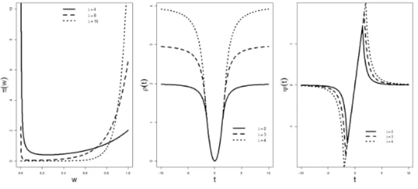
is equivalent to a corresponding posterior mode ofβββ andw. In the left panel of Figure II.1, we plot three sample curves ofπ(wi) forλ20= 4,8,15. It is observed that,wi = 1
with a large probability for a large λ20, and wi = 0with a large probability for a small
λ20. The convexity ofπ(wi)between 0and 1justifies the outlier detection ability of
the PAWLS in (II.3) from a Bayesian perspective.
II.2.1. A General Threshold Rule and Its Link to Sparse M-estimation
In fact, the PAWLS with Lasso in (II.3) can be generalized to a series of weight shrinkage estimation which enjoys strong robustness. To understand this property, we first define a class of scaleshrinkage rule as follows.
Definition II.1. (Scale Threshold Function) For any threshold parameter λ >0, a positive function Θλ(t), t∈R is defined to be a scale threshold function if it satisfies
(1) (Symmetric) Θλ(t) = Θλ(−t) ,
(2) (Non-increasing)Θλ(t)≥Θλ(t0) for 0≤t ≤t0 and
(3) (Two extremes) lim
t→0Θλ(t) = 1 and tlim→∞Θλ(t) = 0.
The scale threshold function in Definition II.1 shares the similar spirit as one in [SO12], but these two types threshold functions have different features. Specifically,
Θλ(·) here is designed to shrink any small positive values (close to 0) to 1, while the
one in [SO12] is to shrink any large values to0. Based upon the above scale shrinkage rule, we can establish an interesting connection between the PAWLS estimation and the sparse M-estimation. Such a connection explains strong robustness properties of the proposed PAWLS in (II.3).
Figure II.1. Display of Some Functions. Left: The Shape of πλ(wi) Function with
λ= 4,8,15; Middle: The ρλ Function with Tuning Parameter λ= 2,3,4; Right: The
ψλ Function with Tuning Parameter λ = 2,3,4
Theorem II.2. Suppose βββ˜ = ˜βββ(0,w˜) is a solution in (II.2) for λ1n = 0 and we
2 i = Θλ(yi−xiβββ˜), 1≤i≤n. Here Θλ(·) for some λ >0 is a threshold function defined in
Definition II.1. Thenβββ˜ is also an M-estimator such thatβββ˜ = argminβββ∈Rp
Pn
i=1ρλ(yi− x0iβββ). In particular, ψλ(t) = dρλ(t)dt satisfies,
ψλ(t) =tΘλ(t). (II.4)
The proof of Theorem II.2 is given in Appendix. Theorem II.2 tells us that a weight generated from any given scale threshold rule can be linked to a corresponding M-estimator. For example, the PAWLS with the Lasso in (II.3) indicates that wˆi =
{nλ2n/(yi−x0iβββˆ)2} ∧1. Thus, if we let λ = nλ2n, then the scale shrinkage rule for
(II.3) becomes
Θλ(t) =
(
λ2/t4 if t2 > λ,
From Theorem II.2, the PAWLS estimation in (II.3) is linked to a corresponding sparse M-estimator with ψ function with
ψλ(t) =
(
λ2/t3 if t2 > λ,
t if t2 ≤λ, (II.6)
and the corresponding ρ function, ρλ(t) =
(
−λ2/(2t2) +λ, if t2 > λ,
t2/2, if t2 ≤λ. (II.7)
See the middle and right panels in Figure II.1 for three curves ofρλ(t)andψλ(t)under
λ = 2,3,4. Notice that lim
t→∞ψλ(t) = 0 and tlim→∞ρλ(t) = λ. Thus the ρ function in (II.7) gives a weakly redescending M estimation with strong robustness. Naturally, the PAWLS solution in (II.3) can be understand as a regularized robust M-estimator with the Lasso penalty. From now on, our investigation is focused on this particular PAWLS estimator. Without being addressed in particular, the Lasso penalty is used in the PAWLS approach.
II.3. Implementation
II.3.1. Coordinate Decent Algorithm for PAWLS
We first notice that (II.3) is not a convex optimization problem. This is not surprising due to the link to a regularized redescending M estimator and strong robustness discussed in Section II.2.1. However, for a given w, the function ofβββ is a convex optimization problem, and the vice versa. Therefore, the objective function (II.3) is a bi-convex function. This biconvexity guarantees that the algorithm has promising convergence properties [GPK07]. We can compute a PAWLS estimate efficiently in Algorithm 1 using coordinate decent algorithm [GPK07].
For each pair of (λ1n, λ2n), those initialization valuesβββ(1),w(1) play important