Mid-Price Movement Prediction in Limit Order Books Using Feature Engineering and Machine Learning

(1)

Mid-Price Movement Prediction

in Limit Order Books Using

Feature Engineering and

Machine Learning

(2)

(3)

7DPSHUH8QLYHUVLW\'LVVHUWDWLRQV $'$0$17,2617$.$5,6

0LG3ULFH0RYHPHQW3UHGLFWLRQ

LQ/LPLW2UGHU%RRNV8VLQJ

)HDWXUH(QJLQHHULQJDQG

0DFKLQH/HDUQLQJ

$&$'(0,&',66(57$7,21 7REHSUHVHQWHGZLWKWKHSHUPLVVLRQRI WKH)DFXOW\RI,QIRUPDWLRQ7HFKQRORJ\DQG&RPPXQLFDWLRQ6FLHQFHV RI7DPSHUH8QLYHUVLW\ IRUSXEOLFGLVFXVVLRQLQWKH/HFWXUHURRP7% RIWKH7LHWRWDOREXLOGLQJ.RUNHDNRXOXQNDWX7DPSHUH

(4)

$&$'(0,&',66(57$7,21 7DPSHUH8QLYHUVLW\ )DFXOW\RI,QIRUPDWLRQ7HFKQRORJ\DQG&RPPXQLFDWLRQ6FLHQFHV )LQODQG Responsible supervisor and Custos 3URIHVVRU 0RQFHI*DEERXM 7DPSHUH8QLYHUVLW\ )LQODQG Supervisors 3URIHVVRU -XKR.DQQLDLQHQ 7DPSHUH8QLYHUVLW\ )LQODQG $GMXQFW3URIHVVRU $OH[DQGURV,RVLILGLV 7DPSHUH8QLYHUVLW\ )LQODQG $VVRFLDWH3URIHVVRU $DUKXV8QLYHUVLW\ 'HQPDUN Pre-examiners 3URIHVVRU $OHF1.HUFKHYDO )ORULGD6WDWH8QLYHUVLW\ 86$ $VVRFLDWH3URIHVVRU 3HNND0DOR $DOWR8QLYHUVLW\ )LQODQG Opponent 3URIHVVRU 3HWHU6DUOLQ +DQNHQ6FKRRORI(FRQRPLFV )LQODQG 7KHRULJLQDOLW\RIWKLVWKHVLVKDVEHHQFKHFNHGXVLQJWKH7XUQLWLQ2ULJLQDOLW\&KHFNVHUYLFH &RS\ULJKW$GDPDQWLRV1WDNDULV &RYHUGHVLJQ5RLKX,QF ,6%1SULQW ,6%1SGI ,661SULQW ,661SGI KWWSXUQIL851,6%1 3XQD0XVWD2\±<OLRSLVWRSDLQR 7DPSHUH

(5)

(6)

(7)

ABSTRACT

The increasing complexity of financial trading in recent years revealed the need for methods that can capture its underlying dynamics. An efficient way to organize this chaotic system is by contracting limit order book ordering mechanisms that operate under price and time filters. Limit order book can be analyzed using linear and non-linear models.

The thesis develops novel methods for the identification of limit order book char-acteristics which provide traders and market makers an information edge in their trading. A good proxy for traders and market makers is the prediction of mid-price movement, which is the main target of this thesis. The contributions of this thesis are categorized chronologically into three parts. The first part refers to the intro-duction in the literature of the first publicly available limit order book dataset for high-frequency trading for the task of mid-price movement prediction. This dataset comes together with the development of an experimental protocol that utilizes meth-ods inspired by ridge regression and a single layer feed-forward neural network as classifiers. These classifiers use state-of-the-art limit order book features as inputs for the target task.

The next contribution of this thesis is the use and development of a wide range of technical and quantitative indicators for the task of mid-price movement predic-tion via an extensive feature selecpredic-tion process. This feature selecpredic-tion process iden-tiﬁes which features improve predictability performance. The results suggest that the newly introduced quantitative feature based on an adaptive logistic regression model for online learning was selected ﬁrst according to several criteria. These crite-ria operate according to entropy, linear discriminant analysis, and least mean square error.

The third contribution is the introduction of econometric features as inputs to deep learning models for the task of mid-price movement prediction. An extensive comparison against other state-of-the-art hand-crafted features and fully automated

(8)

feature extraction processes is provided. Furthermore, a new experimental proto-col is developed for the task of mid-price prediction, to overcome the problem of time irregularities, which characterizes high-frequency data. Results suggest that ad-vanced hand-crafted features such as econometric indicators can predict movements of proxies, such as mid-price.

(9)

PREFACE

The work presented in this thesis has been carried out at Tampere University, Fin-land, during the years 2016-2019.

First and foremost, I would like to thank my supervisor, Professor Moncef Gabbouj, for his endless support, patience, and help throughout this project. His academic genius and rigorous teaching have not only been invaluable but also inspirational. I would also like to thank my second supervisor Professor Juho Kanniainen, for his constant support as well as his technical supervision for the numerous researches that we have conducted.

I would also like to acknowledge a special debt to my advisor and immensely tal-ented Professor Alexandros Iosiﬁdis, who helped me to run the extra mile during this project.

I also gratefully acknowledge the funding that I received from Marie Sklodowska-Curie Innovative Training Network for the entire duration of my Ph.D. studies. To my co-authors, Giorgio Mirone and Martin Magris: thank you for your gen-erous collaboration on our shared projects. I would also like to thank BigDataFi-nance ESRs, MUVIS group researchers, Milla Mäkinen, Jaakko Valli, Kestutis Bal-takys, Milla Siikanen, Jenni Raitoharju, Nikolaos Passalis, Vivi Nousi, Avraam Tsan-tekidis, and George Kanellis for all the discussions we had during these three years of my doctoral education.

I also want to express my profound appreciation to my colleague, Morteza Zabihi, for his help.

My family deserves all the credits as the steady base that has given me the spiritual and material means to accomplish my goals. I feel deeply grateful to my parents,

(10)

Maroula and Yannis, as well as my grandparents, Despina and Kostas. My sister and my best friend, Dr. Virginia Dakari, has always been there for me, believing in me and cheering me up at times when I felt my courage failing. As for my Alina, for her enduring love, affection, and sunny optimism, I thank her deeply.

(11)

2.5 SLFN example with several input units (left), one hidden layer (mid-dle) and an output layer with four units(right)[P1]. . . 34 2.6 MLP with two hidden layers (the graph was created in NN-SVG). . . 35 2.7 Example of a basic CNN architect (the graph was created in NN-SVG) 36 2.8 LSTM internal structure which shows how the information ﬂows

through gates. . . 39 2.9 Example of a symmetrical undercomplete AE . . . 47 3.1 Experimental Setup Framework based on an Anchored Forward

cross-validation format ([P1]). . . 52 3.2 Experimental Setup Framework based on independent feature blocks

(i.e.,t₁, ...,t₁₀, t₁₁, ...,t₂₀, ..., etc) format. This format constructs the input feature representations (FR) ([P3]). . . 53

3.3 Experimental Setup Framework based on online learning format ([P3]).

(14)

4.1 Bar plots with variance present the average (i.e. average F1 perfor-mance for the 9-fold protocol for all the features) F1 score of the 12 different models for the cases of 5, 50, 100, 200, and 273 number of best features. The order of the models from the left to the right col-umn is (1) feature list sorted based on entropy and classified based on LMS, (2) feature list sorted based on LMS1 and classified based on LMS, (3) feature list sorted based on LMS2 and classified based on LMS, (4) feature list sorted based on LDA1 and classified based on LDA, (5) feature list sorted based on LDA2 and classified based on LDA, (6) feature list sorted based on LDA1 and classified based on LMS, (7) feature list sorted based on LDA2 and classified based on LMS, (8) feature list sorted based on LDA2 and classified based on LMS, (9) feature list sorted based on entropy and classified based on RBFN, (10) feature list sorted based on LMS2 and classified based on RBFN, (11) feature list sorted based on LDA1 and classified based on RBFN, and (12) feature list sorted based on LDA2 and classified based on RBFN ([P2]). . . 67 4.2 F1 (left column plots) and RMSE (right column plots) scores for the

(15)

List of Tables

2.1 Amazon’s message list example from 11:27:45:289 to 11:27:45:305 on 22.09.15, where time is expressed in UNIX format and price is

mul-tiplied by 10,000 . . . 24

2.2 LOB feature sets (obtained from[P1]) . . . 40

3.1 Nordic Stocks . . . 49

3.2 Trading activity of the ﬁve Nordic stocks . . . 50

3.3 US Stocks . . . 50

3.4 Trading activity of the two US stocks . . . 50

4.1 HF Dataset Examples ([P1]) . . . 58

4.2 Results based on Unﬁltered Representations ([P1]) . . . 59

4.3 Results based on Z-score Normalization ([P1]) . . . 59

4.4 Feature list of the three groups (description and calculations in[P2]). 61 4.5 List of the ﬁrst 10 best features for the 5 sorting methods ([P2]) . . . . 66

4.6 Feature list of the three feature sets: Description for the newly in-troduced, Econometrics-based, handcrafted features can be found in [P3]; where description for the Tech & Quant and LOB feature sets can be found in[P2] . . . 69

(16)

List of Symbols

A Reaction-Diffusion Particle

α Limit Orders Arrival Rate

A(t) Set Of Sell Orders

B(t) Set Of Buy Orders

B Reaction-Diffusion Particle

C_it LSTM’s Cell Gate

e(i) _{Error Function at time instance}_i

E[·] Expected Value

ft

i LSTM’s Forget Gate f_T(t) Poisson Process at time t

ˆ

f_h(·) Kernel Density Function

gt

i LSTM’s Input Gate

h Activation’s Function Vectors

h Bandwidth

H† _{Moore-Penrose Pseudoinverse Matrix} H Network’s Hidden Layer Outputs Matrix

h_t LSTM’s Hidden State Output

k Time Series Lag

l_x Maximal Output Value

nb₍_·₎ _{Bid-Side Depth} na₍_·₎ _{Ask-Side Depth} ot

i LSTM’s Output Gate o Neural Network Output

pa

x− Before Change Ask Price p_x New Order’s Price

p_xb₋ Before Change Bid Price

pa_x New Ask Price

pb

x New Bid Price pa

j Ask Agent’s LOB Price pb

j Bid Agent’s LOB Price

¯

p Upper Bounded Price Particle

(17)

R_i Stationarity Process ˜

R_i Stationarity Process After Price Change

S Random Variable

t_x New Order’s Arrival Time

T Targetst_iMatrix

t_i Target Vector At Time Instance

va

x− Before Change Ask Volume vb

x− Before Change Bid Volume Vb

x− Before Change Bid Volume v_t New Order’s Volume

Va

x− Before Change Ask Volume Va

x New Ask Volume Order V_xb New Bid Volume Order

V Hidden’s Layer Weights

W Weights’ Matrix

X Time Series

X Samplesx_iMatrix

x_i Sample At Time Instancei

x New Orders

x_i Set Of Vectors

Z(t) Statistical Criterion

z Cut-off Point

Δp(t) Price Variation At Time t

η Market Orders Arrival Rate

λ Regularization Penalty

μ Mean

π Tick Size

σ Smallest Traded Amount

σg Sigmoid Function σ2

z Constant Variance

(18)

List of Abbreviations

ADX Average Directional Index AE Autoencoder

CNN Convolutional Neural Network DM Directional Movement

EG Engle-Granger Statistical Test ELM Extreme Learning Machine FN False Negatives

FP False Positives

FR Feature Representation HF High Frequency

i.i.d. Independent and Identical Distributed IV Integrated Variance

LDA Linear Discriminant Analysis LMS Least Mean Squares

LOB Limit Order Book LRL Linear Regression Line LSTM Long Short-Term Memory MB Message Book

MLP Multilayer Perceptron PA Pre-averaged Variance QV Quadratic Variation

RBFN Radial Basis Function Neural Network ReLU Rectiﬁed Linear Activation Function RK Realized Kernel

RMSE Root Mean Squared Error RNN Recurrent Neural Network RV Realized Variance

RR Ridge Regression SAR Stop And Reverse

SLFN Single-Hidden Layer Feedforward Neural Network TF True Negatives

TP True Positives TR True Range

(19)

LIST OF PUBLICATIONS

[P 1] A. Ntakaris, M. Magris, J. Kanniainen, M. Gabbouj and A. Iosiﬁdis.

Bench-mark dataset for mid-price forecasting of limit order book data with machine

learning methods.Journal of Forecasting37.8 (2018), 852–866.

[P 2] A. Ntakaris, J. Kanniainen, M. Gabbouj and A. Iosiﬁdis. Mid-Price

Predic-tion Based on Machine Learning Methods with Technical and Quantitative

Indicators.PLOS ONE(under review).

[P 3] A. Ntakaris, G. Mirone, J. Kanniainen, M. Gabbouj and A. Iosiﬁdis.

Fea-ture Engineering for Mid-Price Prediction With Deep Learning.IEEE Access

7 (2019), 82390–82412.

Preliminary results of[P1]were presented at the 10t h International Conference on

Computational and Financial Econometrics (CFE 2016)in Seville, Spain, on

(20)

(21)

1 INTRODUCTION

Trading started several centuries ago. The Dutch East India was the ﬁrst publicly traded company in 1602, while the New York Stock Exchange (NYSE) was created in 1817 and became the most dominant stock ex-change in the USA. Nasdaq, the second-biggest stock exchange after NYSE, was founded in 1971 and acquired other

stock exchanges such as the Finnish stock exchange in Helsinki1in 2003. However,

it was not until 1967 that electronic trading platforms were introduced as an alterna-tive trading system by Instinet in New York. Since then, electronic and automated trading increased their impact on the trading ﬂoor and nowadays, this type of trad-ing is the only possible way to exchange stocks. Electronic platforms created a very complex and remarkably fast system which offers instant access to several stock ex-changes. This dynamic system is able to trade large volumes in milliseconds or even nanoseconds. Transaction speed and complexity of this trading universe created the need for efﬁcient analysis of its dynamics.

One way to formulate and organize such a complex system is the so-called limit order book (LOB). LOB is the way that stock exchanges organize their trading ac-tivity. It is a mechanism that sorts trades on a price-time sequence, which means that LOB prioritizes orders ﬁrst according to the price level and next according to arrival time. LOB has two sides: the ask side and the bid side. Ask refers to the minimum price someone is willing to sell a given stock at, while bid refers to the maximum price that someone is willing to pay for a stock. Every LOB’s ask and bid side is divided into several price levels. Every price level comes together with the

volume/number of available stock pieces. Both LOB sides (i.e., ask and bid) have

their best ask and bid prices, respectively. The average of the best ask and bid price constitutes the so-called mid-price. Even though mid-price cannot be traded directly, many investors use it as a proxy to identify potential movements of the actual ask and bid stock prices.

(22)

Movement prediction of proxies like LOB’s mid-price is a challenging task due to several reasons such as data complexity and availability, identiﬁcation of factors that explain the source of uncertainty, and assumption elimination of every possi-ble underline process. Another challenge that makes LOB’s mid-price movement prediction even more complicated is the size of intraday trading activity in a high-frequency environment. Under these challenges, a critical question arises: is LOB’s mid-price predictable? The present thesis proposes a coherent answer to this ques-tion by connecting machine and deep learning methods with state-of-the-art feature engineering as part of several experimental protocols.

Machine and deep learning methods are capable of analyzing linear and non-linear complex systems. An example of a complex system is the LOB. Such methods were extensively used in image and video applications for data parsing (e.g., filtering) via numerous model options, mainly based on functions-kernels used for classifica-tion or predicclassifica-tion. Machine and deep learning aim to learn from the data (e.g., LOB dataset), and, together with recent computational advancements, they offer efficient analysis methods for financial applications, such as mid-price movement prediction. Besides their ability to learn from data, these methods are competent enough to uti-lize representations effectively as inputs. These inputs are usually handcrafted fea-tures, and their purpose is to transform raw data into meaningful signals. That being said, development of state-of-the-art handcrafted features comes with challenges as they require an in-depth analysis of data and understanding of any underlying pro-cess that may be attached to it.

In this thesis, such in-depth analysis is proposed as a result of the extensive ex-perimental basis for the task of LOB’s mid-price movement prediction. First, an experimental protocol for high-frequency LOB data is developed and made publicly available. What is more, state-of-the-art LOB hand-crafted features and linear and non-linear classiﬁers utilized and developed for LOB dynamics analysis. The solu-tions have proven that mid-price’s movements can be predictable. Next, feature en-gineering exploitation based on technical and quantitative indicators as extensions of the existing LOB features provides insight via an extensive study, whose features are suitable for the task of mid-price movement prediction. This study is based on the conversion of entropy, linear discriminant analysis, and least mean square as feature sorting methods. This analysis reveals that mid-price movements could be predicted by means of the best subset selection of advanced hand-crafted features. Last, one

(23)

more hand-crafted econometric-based feature set is presented as input to a wide range of deep learning models. Its aim is to offer a fair evaluation against LOB, technical, quantitative and fully automated features. The output of this analysis led to highly accurate estimation of when the next mid-price movement will happen.

1.1 Objectives and Outline of the Thesis

In this thesis, the focus is placed on capturing, via feature engineering, LOB dynam-ics by utilizing machine and deep learning methods. The objectives of this thesis addressing the research problem stated above are the following:

• To investigate whether state-of-the-art features can predict, with the use of ma-chine learning models, mid-price movements based on high-frequency LOB data.

• To develop state-of-the-art handcrafted features and scrutinize their effective-ness for the task of mid-price movement prediction through the development of experimental protocols which they can be publicly available.

• To determine the effectiveness of deep learning for online mid-price movement

prediction via feature engineering.

The thesis is organized as follows. In Chapter 2 an overview of the key concepts of interest are provided. This background section contains the main ideas of High-frequency (HF) Data properties (Section 2.1), Limit Order Books (Section 2.2), Ma-chine and Deep Learning (Section 2.3), and Feature Engineering (Section 2.4). Chap-ter 3 presents the datasets, experimental protocols and metrics used in the analysis. The contributions of this thesis are discussed in Chapter 4. Section 4.1 presents a novel approach to predicting mid-price movements based on state-of-the-art hand-crafted features. In Section 4.2 an extensive analysis for feature engineering is de-veloped together with a novel set of handcrafted features for online learning for the task of mid-price movement prediction. In Section 4.3 the development of econo-metric features for deep learning is introduced via an experimental protocol suitable for online learning for the task of mid-price movement prediction. Finally, Chap-ter 5 summarizes the most important ﬁndings of the thesis along with concluding remarks and topics for future research.

(24)

1.2 Publications and Author’s Contribution

In[P1], a benchmark LOB dataset was published for the task of mid-price movement

prediction. The major contribution of this paper is the very ﬁrst detailed experimen-tal protocol for a LOB benchmark dataset based on Nordic stocks. State-of-the-art handcrafted features were tested through linear and non-linear classiﬁers for the pre-diction of several projected horizons of future mid-price movements. Baseline mod-els set up on ridge regression and a single-hidden layer feedforward neural network (SLFN) with k-means were suggested in this task. The candidate is the main author of the publication and is responsible for developing and implementing the suggested models and protocol as well as writing the initial draft of the paper.

In [P2], an extensive feature selection evaluation was performed for the task of mid-price prediction. The evaluation was based on the majority of technical indi-cators together with quantitative indiindi-cators and LOB features. Under a wrapper method, the best sets of features were suggested as optimal selection for the classiﬁ-cation task of mid-price movement prediction. Three methods, entropy, linear dis-criminant analysis (LDA), and least mean squares (LMS), converted into feature se-lection criteria where the majority of them selected ﬁrst the newly introduced adap-tive logistic regression feature. Testing the majority of basic and advanced technical indicators, the development of an adaptive logistic feature and the conversions of en-tropy, LDA, and LMS as feature selection criteria constitue the main contribution of this publication. The candidate developed and implemented the suggested models and protocol and wrote the initial draft of the paper.

In[P3], econometrics features were suggested as inputs to several deep learning models, like multilayer perceptrons (MLP), convolutional neural networks (CNN), and long short-term memory (LSTM) neural networks, for the task of mid-price movement prediction. Introduction of econometrics features is one the main con-tributions of this publication since they performed, in some cases, much better than technical, quantitative, LOB and fully automated features. Another contribution of this publication is the development of a new experimental protocol to overcome the problem of time irregularities of HF data. The candidate is the ﬁrst author of this publication and is responsible for developing and implementing the suggested models and protocol. He also wrote the ﬁrst draft of the paper.

(25)

2 BACKGROUND WORK

This thesis introduces feature engineering for LOB high-frequency trading data by utilizing machine and deep learning for the task of mid-price movement prediction. We will ﬁrst introduce the main concepts of High-Frequency Data, Limit Order Book, Feature Engineering, and Machine and Deep Learning.

2.1 High Frequency Data

Algorithmic trading is a computer-based trading mechanism of selling and buying stocks depending on computerized instructions. High-frequency trading is a type of algorithmic trading that operates under low-latency setting. This low-latency set-ting refers to a system that operates under a single digit millisecond round-trip time

for a packet of data/orders. These data packets, named high-frequency data,

pro-vide records of the intraday trading activity (i.e., message book (MB)). These records contain information regarding:

• Security’s ID code

• Timestamp

• Price

• Volume

• Side (Ask or Bid)

• Type of Order (Submission, Cancellation, Execution)

• Full or Partial Cancellation or Execution

These details are an example (e.g., Table 2.1) of the available trading information and can be extended according to the level of the subscription fee. The ﬂow of intraday information creates the need for analysis of its dynamics.

(26)

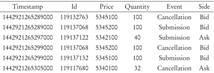
Table 2.1 Amazon’s message list example from 11:27:45:289 to 11:27:45:305 on 22.09.15, where time is expressed in UNIX

format and price is multiplied by 10,000

Timestamp Id Price Quantity Event Side 1442921265289000 119132763 5345100 100 Cancellation Bid 1442921265289000 119137068 5345200 100 Submission Bid 1442921265297000 119137122 5342100 40 Submission Ask 1442921265299000 119137068 5345200 100 Cancellation Bid 1442921265299000 119137132 5345100 100 Submission Bid 1442921265305000 119117680 5340100 32 Cancellation Ask

2.1.1 High-Frequency Data Properties

High-frequency data creates the need for analysis due to its complex nature and dynamics. The analysis can be based on the following general properties of high-frequency data:

• Negative Autocorrelation

Asset’s returns1in a high frequency environment exhibit negative ﬁrst-order

autocorrelation. Autocorrelation measures the correlation between a time

series with a lagged version of itself. More speciﬁcally, for anN-sample time

series X={x₁,x₂, ...,x_N} ∈N ofN samples the autocorrelation with lag k at time instanceiis deﬁned as:

r_X_,_k= E[(xi−μ)(xi+k−μ)] E[(x_i−μ)2_]_E_[(_x

i+k−μ)2]

(2.1) whereE[(x_i−μ)(x_i₊_k−μ)]is the covariance between the time series and its lagged version, and E[(x_i−μ)2_] _and _E_[(_x

i+k −μ)2] are the corresponding variances.

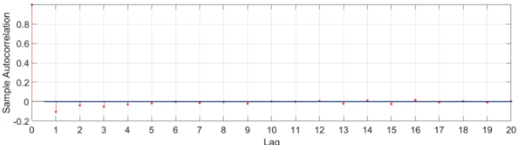
Many authors (e.g. [3],[15],[28]) found evidence of the existence of negative autocorrelation in high-frequency data. An example of the presence of nega-tive correlation can be seen in Figure 2.1 which is based on Amazon trading on 9/22/2015. One can clearly see the presence of negative ﬁrst-order (i.e., lag 1) autocerralation which gradually disappears as the lag increases.

(27)

Figure 2.1 Correlogram up to 20 lags based on Amazon returns for the trading session on 9/22/15. Correlogram shows the existence of negative ﬁrst-order autocorrelation with tight conﬁdence

intervals (blue lines).

• Absence of Normality or Lognormality with Heavy Tails

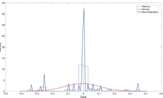
Stock prices in ﬁnancial markets follow a lognormal distribution (e.g., [49]) under the condition that sequential price changes are normally distributed. This does not hold for the case of high-frequency data where the differenc-ing interval2_{becomes shorter (e.g.,}_[₃_]_,_[₁₅_]_,_[₂₄_]_{) and data loses its} normal-ity in the case of a heavy tailed distribution. Figure 2.2 shows that returns’ histograms are not normally distributed and a non-parametric statistical dis-tribution describes better the data (i.e., stock returns). The non-parametric statistical distribution is based on the following kernel density estimator:

ˆ f_h(x) = 1 N h N i=1 K _x₋_x i h (2.2) wherehis the bandwidth adjusted to the data (i.e., Amazon returns) andK(·)is the Gaussian kernel smoothing functionK(x,x_i) =e−(x−xi)

2

2h2 _{. Heavy tails can}

be seen in Figure 2.3, where a Q-Q3provides evidence regarding the existence

of heavy tails in both extremes. • Bid-Ask Bounce

Bid and ask data arrive asynchronously, which means that the quoting process is exposed to noise. The quoting process in tick-by-tick data that creates the bid-ask spread, which is the difference between the bid quote and the ask quote 2_{Differencing interval is deﬁned as the space between two consecutive data points.}

3_{Q-Q (i.e., Quantile-Quantile) plot compares the quantiles of a given dataset and a set of quantiles}

(28)

Figure 2.2 High-frequency data-based Amazon returns can be better described by a non-parametric distribution compared to the normal distribution.

Figure 2.3 Q-Q plot of Amazon returns against normal distribution where presence of heavy tails is obvious in both extremes.

at any time. Bid-ask spread plays a critical role in stock price forecasting since it exhibits a different behavior in liquid and illiquid stocks (i.e., liquid stocks

(29)

have a smaller bid-ask spread compared to illiquid stocks where the spread is higher). This spread represents the proﬁt and some commission fees market maker ﬁrms make. This spread creates room for the bid-ask bounce effect. Bid-ask bounce (e.g., Figure 2.4) is the bouncing of any trade between the bid and ask price. This oscillation can lead to bias in high-frequency data

analy-sis. For instance, authors in[33]suggest that the price movement that takes

place inside the bid-ask spread is not an actual price movement but leads to idiosyncratic volatility increase.4

Figure 2.4 Amazon’s intraday (9/22/15) bid-ask spread ﬂuctuations

2.2 Limit Order Book

Modern financial markets operate under a double auction mechanism called limit order book (LOB). LOB accepts two types of orders, limit and market orders. A limit order is an order to sell or buy a stock at a specified price, whereas a market order is traded instantly under the current market price. As a result, LOB acts as a recording mechanism for the unexecuted trading activity where time and price priority are the primary filters for queues creation. These queues represent, at any time t , the price levels of the bid and ask sides and vary according to order arrivals

(30)

and liquidity5_levels.

Orders, following[30], are deﬁned asx= (p_i,v_i,t_t)where p_i,v_i, and t_i repre-sent the price (i.e., bid or ask), the volume and the order submission time at timei, respectively. All orders arrive with sizev_i ∈ {±kσ|k=1, 2, ...}withσthe smallest traded amount6_{. The set of all active orders,}_L₍_t₎_{, is a càdlàg process since for every} new limit orderx, the following holds:x∈L(t_i)andx∈/lim_t_↑_t

xL(t

₎_{. This activity} defines the depth size for every LOB level in both bid and ask sides. The depth size, especially in the best bid and ask level, is a key element for the price formation (see e.g.,[9],[18]). More specifically, the available bid-side depthnb(p,i)(equivalently, the ask-side depthna(p,t)) at timei is defined as:

nb(p,i):=

{x∈B(i)|p_i=p}

v_i (2.3)

whereB(i)is the set of all active buy orders (equivalentlyA(i)is the set of all sell orders).

The depth of each level in both (bid and ask) sides is modiﬁed constantly due to limit orders, market orders, and cancellations. Limit orders increase the size depth while market orders and cancellations remove liquidity from LOB. Instead of follow-ing this tradfollow-ing activity, the trader can handle the bid and ask queues, as presented in

[14], as stationary processes namely(R_i)i≥1after a price increase and(R˜i)i≥1when there is a price decrease for theit hevent. Both stationary processes exhibit the same distribution for the order book depth in case of a price increase or decrease. For instance, in the case of reduced-form model, for a new order or cancellation arrival, in the bid side, of sizeV_ib at time instancet_ibthere are two scenarios:

• ifvb

i−+Vib≥0 then there is no price change and the order will be satisﬁed • ifvb

i−+Vib<0 then the size of the bid level is reduced together with the price by one ’tick’ of sizeπ. Based on the updated ˜R_i= (_R˜b

i, ˜Rai)values for the bid

5_{Liquidity is deﬁned according to three factors: (i) tightness of a liquid market (i.e., the position’s}

alternation cost over a short period of time), (ii) depth (i.e., order-ﬂow innovations for price changes), and (iii) resiliency (i.e. recovering time from random, uninformative shocks)[39].

6_σ _{together with}_π_{, which is the smallest price interval between orders, are the so-called LOB’s}

(31)

and ask side, the new LOB state is: (p_ib,v_ib,v_ia) = (p_ib₋,v_ib₋+V_ib,v_ia₋)_{_vb i−≥−Vib}+ (p b i−−π, ˜Rib, ˜Rai){vb i−<−Vib} (2.4)

whereis the indicator function, pb

i−is the best bid price before the update,

v_ib₋andv_ia₋are the volume sizes for the best bid and ask sides, respectively. In a similar fashion, for a new arrival to the ask side, of sizeVa

i, LOB’s state will be: • ifva

i−+Via≥0 then there is no price change and the order will be satisﬁed • ifv_ia₋+V_ia<0 then the size of the ask level is reduced together and the price

will be increased by one ’tick’ of sizeπ. Based on the updated ˜R_i= (_R˜b i, ˜Rai) values for the bid and ask side, the new LOB state is:

(p_ia,v_ib,v_ia) = (p_ib₋,v_ib₋,v_ia₋+V_ia)_{_va i−≥−Via}+ (p b i−+π, ˜Rbi, ˜Rai){va i−<−Via} (2.5) whereis the indicator function, p_ib₋is the best bid price before the update, vb

i−and via−are the volume sizes for the best bid and ask sides before the up-date, respectively.

2.2.1 Modelling Limit Order Book Dynamics

The constant LOB state updates create a dynamical system that has attracted the at-tention of many researchers and practitioners. Modeling of LOB dynamics is based on the assumptions that must be proven by the data. Several models have been sug-gested as potential solutions to the description of LOB dynamics.

Cut-Off Strategies

Driven mainly by statistics which are related toL(t)and order ﬂow.7Cut-off strate-gies formulate a decision-making trading approach. The main idea behind this type of modeling is close to a statistical hypothesis test. For instance, following[30], a trader will place an order when the spread8is smaller than 5π. Usually, this type of LOB modeling exhibits the difference between informed and uninformed traders.

7_{Limit orders, together with market orders and cancellations, are the critical components of the}

so-called order ﬂow.

(32)

DeﬁnitionA cut-off strategy, between decisions D₁and D₂, is deﬁned according to the comparison of a statistic Z(t)and a cut-off point z:

D₁, i f Z(t)≤z,

D₂, ot he r wi s e. (2.6)

Diffusion Models

Diffusion models belong to a modeling approach where the arrival of orders, can-cellations, and executions are described by a stochastic process. More specifically, the first model of this type was introduced by[5], where the authors suggested that the interaction between order flow and LOB follows the reaction-diffusion model

A+B → in Physics. These two types of particles are inserted in a pipe of size ˜p

and move randomly by a step of size one. Every time these two particles collide, they are annihilated, and as a result, two new particles are created. This process can describe orders’ arrivals in the LOB. The authors make the following analogies: 1)

Particle→Orders, 2) Finite Pipe→Order Book, and 3) Collision→Transaction.

They deﬁne the stock price at time t as p(t) ∈ {0, ..., ¯p}, where ¯p is an upper bounded discrete price. Every simulation considers half of the agents in the bid side and the other half in the ask side asking for one share of the stock each:

pb_j(0)∈0,¯p 2 , j=1, ...,N 2 (2.7) and pa_j(0)∈¯p 2, ¯p , j=1, ...,N 2 (2.8)

whereN is the number of noise traders9_{. The trading activity revision at each time}

steptis based on an equal probability of a stock going up or down by one tick size.

As a result, every new price for the agent is:

b i d s i d e:p_jb(t+1) =pb_j ±1

as k s i d e: pa_j(t+1) = pa_j ±1 (2.9)

9_{These are the traders whose current volatility depends on the recent changes in the market and}

(33)

The matching or transaction achieved if exists(i,j)∈ {1, ...,N₂}such that:

p_ib(t+1) =pa_j(t+1). (2.10)

This dynamical system follows, as authors suggest, the price variationΔp(t)at time t as this presented by[6]: Δp(t)∼t14 l nt t₀ 1 2 , (2.11)

where t₀represents the initial trading time. The idea that a reaction-diffusion

ap-proach can model LOB dynamics has some drawbacks. For instance, simulations

suggest a Hurst exponent ofH =1/4 and no fat tails exist in the returns’

distribu-tion.

Continuous-time Models

Continuous-time models’ main idea is that order arrivals (i.e., market orders, limit orders, and cancellations) are independent Poisson processes, as this can be seen in models like [16], [17], [19],[20], [53]. The basic model (i.e., [20]) considers the

order ﬂow and the relevant adjustments toL(t)as a queueing system where:

• market orders arrive in chunks of sizeVm_{at a rate of}_ν_{per unit time,}

• limit orders arrive in chunks of sizeVl _{at a rate of}_α_{per unit time,}

• offers are placed, with a uniform probability, on the price grid{1, ...n}with tick sizeπresolution.

The motivation for choosing independent Poisson processes is their simplicity and the fact that they can describe orders’ arrival independently. Following[27], a Poisson process is an arrival process as deﬁned below:

DeﬁnitionAn arrival process is an increasing sequence of random variables 0<S₁<

S₂<..., with S_i₊₁−S_ibe always a positive random variable.

DeﬁnitionA Poisson process is a renewal10process where the interarrival intervals fol-low an exponential distribution function withω >0and each of the interarrival times T_ihas a density

f_T(t) =ωe−ωt, t ≥0. (2.12)

10_{A renewal process is an arrival process during which the sequence of interarrival times is a sequence}

(34)

This model has several drawbacks since Poisson processes are not able to describe the different arrival rates (i.e., intensity periods of high arrival rates cluster in time) as suggested in[21],[31], and[61].

2.3 Machine and Deep Learning

The recent rise of computational power facilitated fields such as machine and deep learning to grow. Machine learning is an automated process where an algorithm performs a task based on a set of filters and conditions. There are several tasks a machine learning algorithm can solve via supervised or unsupervised learning. A supervised task occurs when the algorithm has access to the so-called ground truth, which is a ’proof’ of an event occurrence11. The second type of tasks machine learn-ing algorithms are suitable for are the ones without ground truth. These methods are based only on the given data and operate according to a self-feedback loop dur-ing the learndur-ing process. Both methods require tundur-ing dependdur-ing on the dataset and the problem under consideration. Many applications (e.g., image and voice recogni-tion, time-series analysis, etc.) are based on big datasets, which demand analysis of their dynamics. The focal point of the present thesis is the use of machine learning methods for time-series analysis under the scope of classification and regression for LOB. The machine learning methods presented in this thesis vary from statistics and regression models to neural networks and deep learning.

2.3.1 Ridge Regression

Ridge regression[54]is based on a linear mapping, expressed by a matrixW∈D×C, that optimally maps a set of vectorsx_i ∈D_, _i₌_{1, . . . ,}_N _{to another set of vectors} (noted as target vectors)t_i∈C,i=1, . . . ,n, by optimizing the following criterion:

W∗=argmi n W n i=1 WTx_i−t_i2₂+λW2, (2.13)

where the matrix notation is:

W∗=argmi n

W

WTX−T2₊_λ_W2_. _(2.14)

(35)

X = [x_i, . . . ,x_n]andT= [t_i, . . . ,t_n]are matrices formed by the samplesx_i and t_i

as columns, respectively, andλis the regularization penalty. Every samplex_i

cor-responds to an event with dimensions of that of the input data (e.g., number of dif-ferent features). For instance, in a three-class classiﬁcation problem, the elements of vectorst_i∈C ₍_C ₌_{3 in this case) take values} _t

i k=1, ifxibelongs to classk, and, ift_{i k}=−1, otherwise. The solution of Eq. 2.14 is given by:

W=XXTX+λI−1TT, (2.15)

or

W=XXT+λI−1XTT, (2.16)

whereIis the identity matrix of appropriate dimensions12. After the calculation of

W, a new (test) samplex∈Dis mapped to its corresponding representation in space

C_{, i.e.} _o₌_WT_x_{, and is classiﬁed according to the maximal value of its projection,} i.e.:

l_x=argmax k

o_k. (2.17)

2.3.2 Single-Hidden Layer Feedforward Neural Network

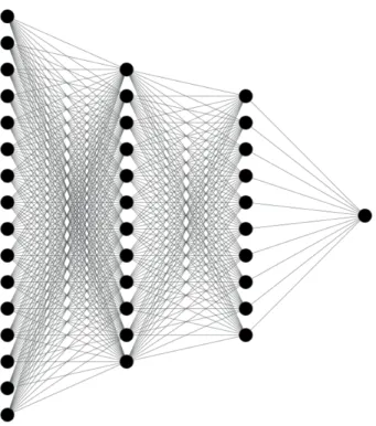
Single-Hidden Layer Feedforward Neural Network (SLFN) is a type of extreme

learning machines (ELM)[35]and belongs to the feedforward type of artiﬁcial neural

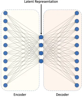
networks. Their topology is based on three layers - input, hidden, and output layers (see Fig. 2.5). SLFN exhibits a good generalization performance and fast learning speed, which makes it suitable for bid datasets.

There are several ways to train this type of neural network. The most common

way is to use the proposed method in[35]where weights of the hidden layers are

determined randomly, but in this thesis, these weights follow[36]where clustering

applied on the training data was used. The clustering is based onK-means algorithm

whereK prototype vectors will be determined, and which are used as the network’s

hidden layer weights.

Since the network’s hidden layer weightsV ∈ D×K _{are ready, the input data}

x_i, i = 1, . . . ,N are non-linearly mapped to vectorsh_i ∈ K_{, expressing the data} 12_{When data is big,}_W_{should be computed using Eq. 2.16, since the calculation of Eq. 2.15 is}

(36)

Figure 2.5 SLFN example with several input units (left), one hidden layer (middle) and an output layer with four units(right) [P1].

representations in the feature space determined by the network’s hidden layer out-putsK_{. Then a radial basis function (RBFN) is used as the activation function, i.e.}

h_i=φRB F(xi), calculated element-wise, as follows: h_{i k}=exp x_i−v_k2₂ 2σ2 , k=1, . . . ,K, (2.18)

whereσis a hyper-parameter denoting the spread of the RBF neuron andv_k

corre-sponds to thek-th column ofV.

The output weightsW∈K×C are subsequently determined by:

W∗=argmi n

W

WTH−T2₊_λ_W2_, _(2.19)

whereH= [h₁, . . . ,h_N]is a matrix formed by the network’s hidden layer outputs for the training data andTis a matrix formed by the network’s target vectorst_i,i= 1, . . . ,n. The network’s output weights will be:

W=HHT +λI−1HTT. (2.20)

After obtaining the network’s parametersVandW, a new (test) samplex∈D_is

mapped to its corresponding representations in spacesK _andC_{, i.e.}_h₌_φ

(37)

ando=WT_h_{, respectively. It is classiﬁed according to the maximal network output,} i.e.: l_x=argmax k o_k. (2.21) 2.3.3 Multilayer Perceptron

Multilayer Perceptron (MLP) ([10],[48],[55]) is a set of functions which ﬁlter the input data in several steps. MLP (see Fig. 2.6 ) is similar to SLFN but with more hidden layers. Every hidden layer consists of nodes that will determine whether the information (i.e., input data from the previous layer) will continue to the next layer. This type of neural network shows a high degree of connectivity, and its weights deﬁne its strength. Usually, an MLP is used for supervised tasks where adjustment of weights takes place via several iterations between the input and the output layers through backpropagation.

Figure 2.6 MLP with two hidden layers (the graph was created in NN-SVG).

One way to train an MLP is to use a sequential data feeding process called batch learning. Batch learning is a process during which the neural network adjusts the

(38)

synaptic weights after the presentation of all the samplesJ={x(i),d(i)}N

i=1in the training process, where: x(i)is the multi-dimensional input vector and d(i) is the

response vector of the supervised problem at instancei where the error function at

instancei is:

e(i)=d(i)−y(i) (2.22)

2.3.4 Convolutional Neural Network

Convolutional neural network (CNN) ([26],[29],[40]) is a type of neural network that exploits spatial correlations between neurons. CNN has the ability to share the so-called tied weights and equivariant representations properties. More speciﬁcally, sparse connectivity can be achieved by using a kernel smaller than the sample input to create a new ﬁltered representation of the given signal. Based on this property, CNN reduces the amount of memory required during training. The second advan-tage that CNN has is the use of tied weights. Tied weights are shared among the inputs since the same amount of weights are applied to the inputs at each layer.

CNN topology varies according to the number of the main building blocks which are: the convolution layer, the pooling layer, and the fully connected layer. An ex-ample of a CNN architecture can be seen in Fig. 2.7.

Figure 2.7 Example of a basic CNN architect (the graph was created in NN-SVG)

The main advantage of CNN is its ability to extract features from the multi-dimensional input signal which is usually expressed as a tensor or matrix. This pro-cess creates linear activations that run via a non-linear activation function (e.g., rec-tiﬁed linear activation function (ReLU), Leaky ReLU, etc). Then a pooling layer

(39)

based on a summary statistic related to the local outputs (e.g., max-pooling) will convert the local output. The last step of the process is the connection to the fully connected layers that will perform the classiﬁcation (or regression) task. This task is based on discrete time series inputs, which formulate the (forward) convolution layer calculation as follows:

y_il+1_,_jl+1_,_d= H i=1 W j=1 D d=1 f_i_,_j_,_d×x_ill+1₊_i_,_jl+1₊_j_,_d (2.23)

whereH,W, andD are the row, columns and depth dimension of the input tensor

x ∈Hl_×_Wl_×_Dl

respectively. f∈Hl_×_Wl_×_Dl

is the ﬁlter bank, and the indexing (il+1₊_i_,_jl+1₊_j_,_d₎_{refers to the iterative local convolution of the ﬁlter bank on the} suggested input for thel-layer. The last step is the use of fully connected layers.

2.3.5 Long Short-Term Memory

Prediction of sequential representations, such as time series, is a common objective in ﬁnance. The presence of temporal behavior of time series needs to be taken into consideration when it comes to model selection. A model which can effectively

man-age these dependencies is long- short-term memory neural (LSTM) network ([25],

[34]). LSTM belongs to the family of recurrent neural networks (RNN) introduced

in[50], which have feedback loops to help identify patterns in the data. LSTM is

an extension of RNN where the difference lies in the fact an LSTM contains sev-eral internal gates that ﬁlter the input information more effectively. The motivation for choosing LSTM is its ability to create connections through time and account for the problem of vanishing (or exploding) gradients. Instead of just applying element-wise non-linear input transformations, LSTM units contain processes which take into consideration the sequential nature of time series. The primary function that explains LSTM’s output is:

h_t= f(h_t₋₁,x_t;η) (2.24)

wherehandxare the state and the input at timet andηare the shared parameters

for a transition function f at time t. LSTM cell is equipped with gates that will

(40)

σg. The ﬁrst pass is the forget gate vector fit: f_i(t)=σg j W_if_,_jh(_jt−1)+ j U_if_,_jx(_jt)+b_if (2.25) where x(_it) andh(_it) are the current input and hidden state vectors of celli at time

t, respectively. The corresponding weight matrices to these vectors are Wf _and

Uf for the forget gate vector withbf the bias term. The next pass is related to the information that is going to be saved to the so-called "cell state". The cell state can

be divided in two parts the input vector and at anhlayer as follows:

C_i(t)= f_i(t)C_i(t−1)+g_i(t)t anh j W_iC_,_jh(_jt−1)+ j U_iC_,_jx(_jt)+b_iC (2.26)

where g(t)is the input gate:

g_i(t)=σ_g

j

W_ig_,_jh(_jt−1)+ j

U_ig_,_jx(_jt)+b_ig (2.27)

The last part is the ﬁltered output. More speciﬁcally, the LSTM output/hidden state

will be formulated by the output gate vectoro_i(t), which can be calculated as follows:

o_i(t)=σ_g

j

W_io_,_jh(_jt−1)+ j

U_io_,_jx(_jt)+b_io (2.28) and the ﬁnal outputh_i(t)is equal to:

h_i(t)=o_i(t)∗t anh(C_i(t)). (2.29)

An example of the internal operations of an LSTM can be seen in Fig. 2.8

2.4 Feature Engineering

Feature engineering is the ﬁeld of study that deals with data analysis and data trans-formation. This study facilitates the process of extracting information relevant to the

problem/task under consideration. There are two main categories for feature

(41)

Figure 2.8 LSTM internal structure which shows how the information ﬂows through gates.

Both categories require in-depth knowledge of data analysis and model development. More speciﬁcally, the former case refers to the process that features a set of vector representation which converts raw data into informative signal based on experts’ opinion, whereas in the latter case a model (e.g., neural network) will extract itself the transformed representations.

Since the problem under consideration in the present thesis focuses on financial data (i.e., the mid-price prediction based on high-frequency data), relevant features/ -factors are related to financial concepts. More specifically, these features will be LOB features, technical indicators, quantitative analysis, econometrics, and fully auto-mated financial processes. The following list of features is by no means exhaustive, demonstrating only a few exemplary cases.

2.4.1 Limit Order Book Features

LOB is an ordering mechanism for the trading activity of the submitted limit and market orders. This trading activity creates a complex system in which relevant

indicators/features should capture its dynamics. The work presented in[38]is an

example of capturing LOB dynamics by handcrafted feature development. LOB features extraction is based on the prediction of mid-price. There are three main categories of feature set whose description can be seen in Table. 2.2

(42)

Table 2.2 LOB feature sets (obtained from [P1])

Feature Set Description Details

Basic u1={Pias k,Vias k,Pib i d,Vib i d}ni=1 10(=n)-level LOB Data Time-Insensitive u2={(Pas ki −Pib i d),(Pias k+Pib i d)/2}ni=1 Spread & Mid-Price

u3={Pnas k−P1as k,P1b i d−Pnb i d,|Pias k+1−Pias k|,|Pib i d+1−Pib i d|}ni+1 Price Differences u4= 1 n n i=1P as k i , 1 n n i=1P b i d i , 1 n n i=1V as k i , 1 n n i=1V b i d i

Price & Volume Means u5= n i=1(P as k i −Pib i d), n i=1(V as k i −Vib i d) Accumulated Differences Time-Sensitive u6= d Pas k i /d t,d Pib i d/d t,dVias k/d t,dVib i d/d t n

i=1 Price & Volume Derivation u7=

λ1

Δt,λ2Δt,λ3Δt,λ4Δt,λ5Δt,λ6Δt

Average Intensity per Type u8= 1_λ1 Δt>λ 1 ΔT ,1_λ2 Δt>λ 2 ΔT ,1_λ3 Δt>λ 3 ΔT ,1_λ4 Δt>λ 4 ΔT ,1_λ5 Δt>λ 5 ΔT ,1_λ6 Δt>λ 6 ΔT

Relative Intensity Comparison u9={dλ1/d t,dλ2/d t,dλ3/d t,dλ4/d t,dλ5/d t,dλ6/d t} Limit Activity Accelaration

These three sets of handcrafted features provide useful insight regarding the evo-lution of price rate changes, or volume rate changes, but they are limited in terms of other LOB characteristics. Several additional factors/features should also be consid-ered, such as volatility estimation, price trends, volume imbalance, etc.

2.4.2 Technical Analysis

Technical analysis is a trading universe where traders make investment predictions based on the idea that stock price is the primary source of information. The cen-tral component of technical analysis is the utilization of charts of volume and price trends. Several indicators developed through the years (e.g., candlestick charts ex-ist since 1600) and fuse with other methods, such as statex-istics. Some examples of technical indicators are:

Average Directional Index

Average directional index (ADX) indicator[56]developed in order to identify the

strength of a current trend. ADX is calculated as follows:

T R=max(H_t−L_t,|Ht−C Lt−1|,|Lt−C Lt−1|) (2.30)

(+DM) =H_t−H_t₋₁ (2.31)

(43)

T R₁₄=T R_t₋₁−(T R_t₋₁/14) +T R (2.33) (+DM₁₄) = (+DL_t₋₁₄)−((+DL_t₋₁₄)/14) + (+DM) (2.34) (−DM14) = (−DLt−14)−((−DLt−14)/14) + (−DM) (2.35) (+DI₁₄) =100×((+DM₁₄)/(+T R₁₄)) (2.36) (−DI14) =100×((−DM14)/(−T R14)) (2.37) DI_{d i f f} 14=|(+DM14)−(−DM14)| (2.38) DI_{s u m}₁₄=|(+DM₁₄) + (−DM₁₄)| (2.39) DX =100×((DI_{d i f f} 14)/(DIs u m14)) (2.40) ADX = (ADX_t₋₁×13) +DX)/14 (2.41)

where: TR is the true range, H_t is the current 10-block’s highest MB price, L_t is

the current 10-block’s lowest MB price,C L_t is the previous 10-block’s closing MB

price,(+DM)is the positive Directional Movement (DM),(−DM)is the negative

DM, T R₁₄ is the TR based on the previous 14-blocks,T R_t₋₁ is the previous TR

price, (+DM₁₄) is DM based on the previous 14 (+DM) blocks, (−DM14) is the

DM based on the previous 14(−DM)blocks,(+DM_t₋₁₄)is the (+DM) of the

pre-vious 14 +DM blocks, DI_{d i f f}

14 is the directional indicator (DI) of the difference between(+DM₁₄) and(−DM14), DIs u m₁₄ is the DI of the sum between(+DM14)

and(−DM₁₄),DX is the directional movement index andADX_t₋₁is the previous

average directional index.

Parabolic Stop and Reverse

(44)

are two main modules for its calculation, the Rising SAR and the Falling SAR, and they are calculated as follows:

• Rising SAR

E P=H_{H i g h}

5 (2.42)

SAR=SAR_t₋₁+AF_t₋₁(E P_t₋₁−SAR_t₋₁) (2.43)

• Falling SAR

E P=L_Low

5 (2.44)

SAR=SAR_t₋₁−AF_t₋₁(E P_t₋₁−SAR_t₋₁) (2.45)

where AF is the acceleration factor, and E P the extreme point with highest high

(H_{H i g h}

5) and lowest low (LLow5) for the last ﬁve 10-MB blocks.

Linear Regression Line

Linear regression line (LRL) is a basic statistical method that provides information for a future projection wherein trading is used to capture overextended price trends. The basic calculation steps are as follows:

PV =c₁+c₂×M B_{p r i c e s} (2.46) c₂=r×(s t d_PV/s t d_{M B} p r i c e s) (2.47) r = 10 i=1(M Bp r i c e s(i)−M Bp r i c e s)(PV(i)−PV) 10 i=1(M Bp r i c e s(i)−M Bp r i c e s) 2₍10 i=1(PV(i)−PV) 2 (2.48) c₁=PV −c₂×M B_{p r i c e s} (2.49)

wherePV are the predicted values, r is the correlation coefﬁcient, andM B_{p r i c e s} and

(45)

2.4.3 Quantitative Analysis

Quantitative analysis ([1],[2]) belongs to a trading universe where a decision is made based on mathematical models and statistics. This type of analysis can effectively be used not only for pattern identiﬁcation in massive datasets but also to mitigate investment risks. One of the goals of the thesis is to use quantitative analysis for pattern recognition. Examples of features that utilize mathematical concepts and statistics follow:

Autocorrelation and Partial Correlation

Autocorrelation and partial correlation [11], [23]are key features in the develop-ment of time series analysis. Under the assumption of stationary stochastic pro-cesses, their local behavior is:

• Autocorrelation

r_X_,_k= E[(xi−μ)(xi+k−μ)] E[(x_i−μ)2_]_E_[(_x

i+k−μ)2]

(2.50) where x_i andx_i₊_k are the time series of lagkat time instancei,μ=E[x_i] =

_∞

−∞x p(x)d x andσ2x=E[(xi−μ)2] =

_∞

−∞(x−μ)2p(x)d x are the constant mean and constant variance, respectively.

• Partial Correlation

– For the general case of an autoregressive modelAR(p), we have:

x_i₊₁=φ1xi+φ2xi−1+...+φpxi−p+1+ξi+1 (2.51) of lag 1 up to pfollows: <x_ix_i₊₁>= p j=1 (φj<xixi−j+1>) (2.52) <x_i₋₁x_i₊₁>= p j=1 (φ_j<x_i₋₁x_i₋_j₊₁>) (2.53) <x_i₋_k₊₁x_i₊₁>= p j=1 (φj<xi−k+1xi−j+1>) (2.54)

(46)

<x_i₋_p₊₁x_i₊₁>= p

j=1

(φj<xi−p+1xi−j+1>) (2.55)

by diving withN−1 and autocovariance of zero separated periods (where

the autocovariance function is even), all the lag periods above will be: r_i=

p

j=1

φjrj−1 (2.56)

where r_i,i = 1, 2, ...,k, ...,p for the matrix operations RRRΦΦΦ = rrr, RRR ∈

p×p_, _ΦΦΦ _∈ p×1 _and _rrr _∈ p×1_{. The symmetric and full rank}_ΦΦΦ _are

as follows: ˆΦΦΦ=RRR−1rrr.

– Yule-Walkerequations calculation for a lagged interval 1ip:

ˆ ΦΦΦ= RRR(i)−1rrr(i)= ⎡ ⎢ ⎢ ⎢ ⎢ ⎢ ⎢ ⎢ ⎣ ˆ φ₁ ˆ φ₂ ... ˆ φi ⎤ ⎥ ⎥ ⎥ ⎥ ⎥ ⎥ ⎥ ⎦ (2.57) Cointegration

Investigation of time-series equilibrium[22],[32]can be tested through the cointe-grated hypothesis. Utilizing the cointegration test will help ML traders avoid the problem of spurious regression. For this reason an Engle-Granger (EG) test is uti-lized for the multivariable case of LOB ask (A_t) and bid (B_t) times series. The for-mulation of the EG test for the ask and bid LOB prices are as follows:

• A_t andB_t ∼I(d), whereI(d)represents the order of integration

• Cointegration equation based on the error term: u_t=A_t−αB_t, where

ordi-nary least squares (OLS) is performed for the estimation ofα

• EG Hypothesis: u(t)∼I(d),d=0

(47)

2.4.4 Econometrics

Econometrics ([46], [51],[59]) is the field of study that covers topics related to fi-nancial applications and assumptions under the scope of statistics and mathemat-ics. This field is vast and covers methods from regression and probability theory to asymptotic theory and volatility estimation. These topics are directly connected to high-frequency financial data, which come with variation in prices, known in the financial literature as volatility. Since the thesis deals with this type of data, some features will be presented in this section as examples of feature engineering under econometric theory.

Volatility Measures

Features based on volatility measures estimate either the integrated variance (IV), that is, the process

IV_t=

t

0

σ2

sds (2.58)

or, more generally, the quadratic variation (QV) [X,X]t = t 0 σ2 sds+ 0<s≤t (ζsdNs)2. (2.59)

Here,X is the logarithmic price of a given asset. Assuming thatX_t follows an Itô

semimartingale; that is, X_t=X₀+ t 0 b_sds+ t 0 σsdWs+ t o ζsdNs, (2.60)