Nonparametric Predictive Inference for System Failure Time

(1)

Durham E-Theses

Nonparametric Predictive Inference for System Failure

Time

AL-NEFAIEE, ABDULLAH,HOMOD,O

How to cite:

AL-NEFAIEE, ABDULLAH,HOMOD,O (2014) Nonparametric Predictive Inference for System Failure Time, Durham theses, Durham University. Available at Durham E-Theses Online:

http://etheses.dur.ac.uk/10877/ Use policy

The full-text may be used and/or reproduced, and given to third parties in any format or medium, without prior permission or charge, for personal research or study, educational, or not-for-prot purposes provided that:

• a full bibliographic reference is made to the original source

• alinkis made to the metadata record in Durham E-Theses

• the full-text is not changed in any way

The full-text must not be sold in any format or medium without the formal permission of the copyright holders. Please consult thefull Durham E-Theses policyfor further details.

(2)

Academic Support Oce, Durham University, University Oce, Old Elvet, Durham DH1 3HP e-mail: [email protected] Tel: +44 0191 334 6107

http://etheses.dur.ac.uk

(3)

Nonparametric Predictive Inference for

System Failure Time

Abdullah H. Al-nefaiee

A thesis presented for the degree of

Doctor of Philosophy

Department of Mathematical Sciences

University of Durham

England

2014

(4)

Dedicated to

my parents

(5)

Nonparametric predictive inference for

system failure times

Abdullah H. Al-nefaiee

Submitted for the degree of Doctor of Philosophy

2014

Abstract

This thesis presents the use of signatures within nonparametric predictive inference (NPI) for the failure time of a coherent system with a single type of components, given failure times of tested components that are exchangeable with those in the system. NPI is based on few modelling assumptions and here leads to lower and upper survival functions. We also illustrate comparison of reliability of two systems, by directly considering the random failure times of the systems. This includes explicit consideration of the difference between failure times of two systems. In this method we assume that the signature is precisely known. In addition, we show how bounds for these lower and upper survival functions can be derived based on limited information about the system structure, which can reduce computational effort substantially for specific inferential questions. It is illustrated how one can base reliability inferences on a partially known signature, assuming that bounds for the probabilities in the signature are available. As a further step in the development of NPI, we present the use of survival signatures within NPI for the failure time of a coherent system which consists of different types of components. It is assumed that, for each type of component, additional components which are exchangeable with those in the system have been tested and their failure times are available. Throughout this thesis we assume that the system is coherent, we start with a system consisting of a single type of components, then we extend for a system consisting of different types of components.

(6)

Declaration

The work in this thesis is based on research carried out at the Department of Mathe-matical Sciences, Durham University, UK. No part of this thesis has been submitted elsewhere for any other degree or qualification and it is all the author’s original work unless referenced to the contrary in the text.

Copyright c 2014 Abdullah H. Al-nefaiee.

“The copyright of this thesis rests with the author. No quotations from it should be published without the author’s prior written consent and information derived from it should be acknowledged”.

(7)

Acknowledgements

I have so much to be thankful for, first and foremost, for Allah the Lord of the universe for the countless blessings he has bestowed on me, both in general and particularly during my work on this thesis.

My main appreciation and special thanks go to my supervisor, Prof. Frank Coolen, for his unlimited support, expert advice and guidance. Without his will-ingness and invaluable suggestions this PhD thesis could not have been completed. I appreciate his high standards, his ability, his knowledge of research methodology. One simply could not wish for a better and more friendly supervisor, which I ap-preciate from my heart. It is really hard to find the words to express my gratitude and appreciation for him.

I am extremely grateful to my parents who gave me everything a son could wish for, including support throughout the writing of this thesis, especially when I needed encouragement.

I want to acknowledge my closest supporters, my beloved wife Wafa, for her confidence and constant encouragement, and my two daughters Tala and Saba, who lighten my life with their smiles and ever present love.

I am also grateful to my brothers and sisters, especially Mohammed, Abdulhade, and Ali, who want the best and success for me, and have been a great source of motivation and support through all these years.

Thanks are also due to my colleagues and my friends who helped me during my numerous challenges. I am indebted for their friendship.

Finally, I wish to thank my country, Saudi Arabia, represented by King Abdullah, for granting me the scholarship and providing me with this great opportunity for completing my studies in the UK and so enabling me to fulfil my ambition.

(8)

Chapter 1 Introduction

1.1 Overview

One of the basic problems in reliability theory is prediction of the failure time of a system consisting of multiple components, each of which has a random failure time. Assessing the reliability of a coherent system requires knowledge about the structure function of the system as well as the probability distribution of component failure times. System reliability can be studied at the structural level by building a relationship between the system reliability and the reliability of its components. Throughout this thesis, we restrict attention to coherent systems, a system is coher-ent if each of its componcoher-ents is relevant and its structure function is monotonously increasing [12].

The theory of system signatures [61] provides a powerful framework for reliability assessment for systems consisting of exchangeable components. For a system withm

components, the signature is a vector containing the probabilities for the events that the system fails at the moment of the j-th ordered component failure time, for all

j = 1, . . . , m. In this thesis, The use of signatures for system reliability is explored

in the generalized theory of uncertainty quantification where lower and upper proba-bilities (also called ‘imprecise probability’ [65] or ‘interval probability’ [67]) are used instead of precise probabilities. This thesis presents the use of signatures within Nonparametric Predictive Inference (NPI), a statistical framework which uses few modelling assumptions enabled by the use of lower and upper probabilities to

(11)

1.2. System signatures 2

tify uncertainty. Mainly, we introduce NPI with the use of signatures to derive lower and upper survival functions for the failure time of systems with exchangeable com-ponents, given failure times of tested components that are exchangeable with those in the system. In addition, comparison of reliability of two systems is presented by directly considering the random failure times of the systems. However, deriving the system signature is computationally complex. We present how limited information about the signature can be used to derive bounds on such lower and upper survival functions and related inferences.

The system survival signature [26] is a generalisation of the system signature to systems with multiple component types. We also present the use of survival signatures within NPI for the failure time of a coherent system, which can consist of different types of components. It is assumed that, for each type of component, additional components which are exchangeable with those in the system have been tested and their failure times are available.

In this thesis the NPI method for the system survival function using the system signature is presented in Chapters 2 and 3, and the NPI method for the system survival function using the survival signature is presented in Chapter 4.

In Section 1.2 we briefly review the concept of system signature. Section 1.3 presents the main idea of NPI. Section 1.4 briefly presents NPI for order statistics of m future real-valued observations given n observations, which will be used in Chapters 2 and 3. Section 1.5 presents a brief overview of NPI for Bernoulli data, which will be used in Chapter 4. Finally, a detailed outline of this thesis is given in Section 1.6, with details of related publications.

1.2 System signatures

In recent decades, system signatures have proven to be a powerful tool for qualifying structures of coherent systems consisting of exchangeable components, which can be used to quantify aspects of reliability of systems such as their failure time distri-bution [61]. Consider a system consisting of components which have exchangeable random failure times [40]. It is convenient to call these ‘exchangeable components’,

(12)

informally they can be said to be all ‘of the same type’. As an example, consider batteries of the same brand; their failure times will not be identical, but not know-ing the individual batteries’ failure times, the exchangeability assumption implies that the information about the failure time of one specific battery is the same as the information about the failure time of any other specific battery. It should be emphasized that such failure times are not statistically independent, as for example learning that one battery’s failure time is small will provide important information about the random failure time of another battery. A standard situation where such an exchangeability assumption is reasonable, and indeed implicit to many standard statistical methods, is when the components (batteries) for which failure times are observed had been chosen by simple random sampling from a batch of components, with interest in predicting the failure times of one or more of the other components from the same batch.

Birnbaum [14] presented the foundations for the study of system reliability via the structure function. For a system with m components, let state vector x = (x1, x2, . . . , xm) ∈ {0,1}m, where for each i, xi = 1 if the ith component functions

andxi = 0 if not. The structure functionφ :{0,1}m → {0,1}is a mapping such that φ(x) = 1 if the system functions and φ(x) = 0 if the system does not function for state vector x. The structure function for series and parallel systems is trivial. The series structure functions only if every component is functioning, while the parallel structure functions as long as at least one component is functioning. The structure function for an m-component series system is given by

φ(x) =

m Y

i=1

xi (1.1)

while for a parallel system it is given by

φ(x) = 1−

m Y

i=1

(1−xi) (1.2)

A system is coherent if each of its components is relevant and its structure function is monotonously increasing. Throughout this thesis we assume that the system is coherent, which means thatφ(x) is not decreasing in any of the components ofx, so system functioning cannot be improved by worse performance of one or more

(13)

of its components. We assume thatφ(0) = 0 and φ(1) = 1, so the system fails if all its components fail and it functions if all its components function [12].

Let the random failure time of a system consisting of m components be TS and

let Tj:m be the j-th order statistic of the m random component failure times, for j = 1, . . . , m, withT1:m ≤T2:m ≤. . .≤Tm:m. The system’s signature [61] is defined

to be them-vectorq with j-th component

qj =P(TS =Tj:m) (1.3)

so qj is the probability that the system failure occurs at the moment of the j-th

component failure. It is natural to assume thatPm

j=1qj = 1; this assumption implies

that the system functions if all components function, has failed if all components have failed, and that system failure can only occur at times of component failures. The essential feature of the calculation of a signature is counting of the orderings of the m potential component failure times that correspond with system failure upon the jth failure time among the m components.

The signature provides a qualitative description of the system structure that can be used in reliability quantification [61]. For example, the survival function of the system failure time can be derived by

P(TS > t) = m X

j=1

qjP(Tj:m > t) (1.4)

and the expected value of TS can be derived by

E(TS) = m X

j=1

qjE(Tj:m) (1.5)

The system signature was introduced by Samaniego in 1985 [60] and has become a useful tool to compute the system reliability [16], and to compare different systems when all components are exchangeable. A comprehensive discussion and an excel-lent review of the results based on system signatures obtained since 1985 and their applications in engineering reliability can be found in a book by Samaniego [61].

In recent years, many authors have discussed theory and applications of system signatures, for example, signatures were used in [52] and [57] to study system com-parison based on stochastic, hazard rate and likelihood ratio orderings. Boland [15]

(14)

presented the signature in terms of the number of path sets in the system as well as the number of ordered cut sets. Andronova et al. [5] applied signatures to a queueing system with an unreliable server. However, signatures have thus far been mostly con-sidered from a probability perspective, not related to statistical inference. The main exception is the recent PhD thesis by Aslett [9], who presents a Bayesian approach for inference on system reliability for several scenarios, with the system structure taken into account through the signature. A particularly interesting feature of his work is the possibility to learn about the system structure in case only system level failure data are available, so without data on individual components. Such inverse inference is useful for black-box systems and requires powerful simulation-based computational methods, for which the Bayesian approach is very suitable. In this thesis, nonparametric predictive inference is used, which provides a frequentist statistics alternative to the Bayesian approach, suitable for inference about system reliability based on failure data for individual components. Throughout the thesis, the system structure is assumed to be known, the presented approach is not suitable for the kind of inverse inferences mentioned above. Knowing the system structure, however, does not necessarily imply that the system signature is readily available, we therefore will also consider inference using only partially known signatures.

Computation of the system signature is a combinatorial exercise. However, this does not mean that it is quite easy, it just means there is a well organized body of knowledge and tools that can be applied to such problems. It is obvious that there are 2 coherent systems of order 2 (series and parallel systems). Shaked and Suarez-Llorens [62] proved that there are 5 different coherent systems consisting of 3 components and 20 different coherent systems consisting of 4 components. They computed the signatures of these systems and used them to study some ordering properties. Navarro and Rubio [56] provide an algorithm to compute the number of coherent systems with a given number of components. They show that there are 180 different coherent systems with 5 components and also computed the signatures of these systems and their expected lifetimes. According to Samaniego [61] the number of coherent systems withm components grows exponentially, there are more than a billion coherent systems with 30 components.

(15)

One may be interested in comparing two systems which do not have the same number of components. Samaniego [61] provides a formula to convert the smaller system into an equivalent larger system with exactly the same failure time distribu-tion as the smaller system. Letq= (q1, . . . , qm) be the signature of a coherent system

withm components which have independent and identically distributed (i.i.d.) fail-ure times. Then the system with m+ 1 components with i.i.d. failure times, with the same distribution as for the smaller system, and with signature

q∗ ₌ m m+ 1q1, 1 m+ 1q1+ m−1 m+ 1q2, 2 m+ 1q2+ m−2 m+ 1q3, . . . , m−1 m+ 1qm−1+ 1 m+ 1qm, m m+ 1qm (1.6)

has identical random system failure time as the system with m components and signature q. Eryilmaz [44] presented an algorithm for computing the signature of consecutive k-out-of-m:F systems, which fail if and only if k of components fail. Such systems have received much attention in the reliability literature in recent years, particularly also with focus on their signatures [45, 55].

Da et al. [48], show how signatures for subsystems can be combined to derive a system’s signature in case of two subsystems in series or parallel configuration, which we will use in Chapter 3. Suppose that the system consists of two subsystemsAand

B with ma and mb components each. Let qa = (q₁a, ..., qmaa) and q

b _{= (}_qb

1, ..., qmbb) be

the signature vectors of subsystems Aand B, respectively. The aim is to derive the signature vectorqof the overall system based on signatures qa_and_qb_{. First consider}

a system which consists of subsystems A and B in parallel configuration. Then the overall system has signature vector q with jth component qj given as follows [48].

Since the system is the parallel of two subsystems, it is clear that the system will not fail at the first component failure, which leads toq1 = 0. For further component

failures, the signature can be derived for the following cases. For 2≤j ≤ma: qj = ma+mb ma −1"j−1 X i=1 j −1 i " qa j−i i X k=1 qb ! ma+mb −j mb −i + qb j−i i X k=1 qa ! ma+mb−j mb−i ## (1.7)

(16)

1.2. System signatures 7 Forma<j ≤mb: qj = ma+mb ma −1" j−1 X i=j−ma qa j−i i X k=1 qb ! j−1 i ma+mb−j mb−i + ma X i=1 qb j−i i X k=1 qa ! j−1 i ma+mb−j mb−i # (1.8) Formb<j ≤ma+mb: qj = ma+mb ma −1" mb X i=j−ma qa j−i i X k=1 qb ! j−1 i ma+mb−j mb−i + ma X i=j−mb qb j−i i X k=1 qa ! j−1 i ma+mb−j mb−i # (1.9)

For a system consisting of subsystems A and B in series configuration, the sys-tem’s signature vectorqhasjth componentqj which can be derived as follows. Since

the system is the series of two subsystems, it is clear that qma+mb = 0. The other

components ofq can be derived for the following cases. For 1≤j ≤ma: qj = ma+mb ma −1"j−1 X i=0 j −1 i " qja−i mb X k=i+1 qb ! ma+mb−j mb−i + qb j−i ma X k=i+1 qa ! ma+mb−j mb−i ## (1.10) Forma<j ≤mb: qj = ma+mb ma −1" j−1 X i=j−ma qa j−i mb X k=i+1 qb ! j −1 i ma+mb−j mb−i + ma−1 X i=0 qb j−i ma X k=i+1 qa ! j −1 i ma+mb−j mb −i # (1.11) Formb<j ≤ma+mb: qj = ma+mb ma −1" mb−1 X i=j−ma qja−i mb X k=i+1 qb ! j −1 i ma+mb−j mb−i + ma−1 X i=j−mb qjb−i ma X k=i+1 qa ! j −1 i ma+mb −j mb −i # (1.12)

(17)

1.3. Nonparametric predictive inference (NPI) 8

1.3 Nonparametric predictive inference (NPI)

Nonparametric predictive inference (NPI) is a statistical approach to learning from data in the absence of prior knowledge, which requires only few modelling assump-tions [21]. NPI gives a direct conditional probability for one or more future ob-servable random quantities, conditional on observed values of related random quan-tities [7, 20, 21]. NPI uses lower and upper probabilities, also known as imprecise probabilities, to quantify uncertainty [8, 30, 65, 67] and has strong consistency prop-erties from frequentist statistics perspective [7, 21]. NPI provides a solution to some explicit goals formulated for objective (Bayesian) inference, which cannot be ob-tained when using precise probabilities [20], and it never leads to results that are in conflict with inferences based on empirical probabilities. Imprecise probabilities provide many exciting opportunities for reliability quantification [31, 63, 64]. The NPI method has already been used for system reliability [1, 23, 37, 53], but only for systems with quite restricted structures. NPI has been developed for a vari-ety of problems in operational research and statistics, including predictive analysis for queueing problems [25], replacement problems [38], and decision making under uncertain utilities [51].

NPI is based on Hill’s assumption A(n) [49] which gives direct probabilities [41]

for one or more real-valued future random quantities, based on observations of n

related random quantities. These probabilities are such that all orderings of the future random quantities among the observed random quantities are equally likely; for more details we refer to Coolen [21]. NPI is a framework of statistical theory and methods that use A(n)-based lower and upper probabilities [30, 31]. In classical

probability theory, a single probability P(E) ∈ [0,1] is used to quantify uncer-tainty about an event E. Lower and upper probabilities generalize the standard theory of (‘single-valued’ or ‘precise’) probability and provide a powerful method for uncertainty quantification [64]. A lower (upper) probability P(E) (P(E)) can be interpreted as supremum buying (infimum selling) price for a gamble on the event

E, or as the maximum lower (minimum upper) bound for the probability of E. An informal way to interpret lower and upper probabilities is as follows; a lower

(18)

prob-1.3. Nonparametric predictive inference (NPI) 9

ability for an eventE reflects the evidence in available information in favour of the event E, the corresponding upper probability for this event reflects the evidence in available information against this event. These are logically linked by the conjugacy propertyP(E) = 1−P(Ec_{), where} _Ec _{is the complementary event to} _E _[30].

To introduce the assumption A(n), we first need to introduce some notation.

Suppose that T1, . . . , Tn, Tn+1 are positive, continuous and exchangeable random

quantities. Let the ordered observations ofT1, . . . , Tn be denoted byt1 < t2 < . . . <

tn. For ease of notation, define t0 = 0 andtn+1 =∞. Thesen observations partition

the non-negative real-line inton+ 1 intervals Ii = (ti−1, ti) for i= 1, . . . , n+ 1. The

assumption A(n) is that the future observation Tn+1, based on n observations, will

fall in the open interval Ii with probability 1/(n+ 1), for each i= 1, . . . , n+ 1,

P(Tn+1 ∈(ti−1, ti)) =

1

n+ 1 (1.13) TheseA(n)-based probabilities are specified for Tn+1, but also hold for any future

observation Tn+i, i ≥ 1, as long as one considers these future observations to be

exchangeable [40]. However, such future observations are not independent [49], learning the value of one of them will change the probabilities for other future observations. Hill [50] discusses A(n) in detail. A(n) does not assume anything else,

and can be considered to be a post-data assumption related to exchangeability. Inferences based on A(n) are predictive and nonparametric, and can be considered

suitable if there is hardly any knowledge about the random quantity of interest, other than the data, which consists of n observations, or if one does not want to use such further information. A(n) is not sufficient to derive precise probabilities

for many events of interest, but it provides optimal bounds for probabilities for all events of interest involving Tn+1.

It should be noted that, to avoid notational complexity, we assume throughout this thesis that there are no tied observations. Any tied observations can be dealt with by breaking ties by adding small values to one or more of the tied observations. The method can be generalized to allow ties by breaking the ties in all possible ways and obtaining the overall NPI lower and upper probabilities as the minimum and maximum, respectively, of the lower and upper probabilities corresponding to each way of breaking the ties [50].

(19)

1.4. NPI for order statistics 10

1.4 NPI for order statistics

For the scenario in Section 1.3, we are now interested in m ≥ 1 future observa-tions, Tn+j for j = 1, . . . , m. We link the data and future observations via Hill’s

assumptionsA(n),A(n+1),. . .,A(n+m−1), see [7,20,27] for more details. Arts et al. [6]

considered NPI for m future observations, and showed that, with Sj = #{Tl ∈ Ii, l = 1, . . . , m}, these assumptions lead to

P( n+1 \ j=1 {Sj =sj}) = n+m n −1 (1.14)

for all (s1, . . . , sn+1) with sj non-negative integers and Pn_j₌₁+1sj = m. For any

event involving the m future observations, Equation 1.14 implies that the number of orderings of them future observations among the n data observations, for which this event holds, can be simply counted as all such orderings have equal probability. Generally in NPI a lower probability for the event of interest is derived by count-ing all ordercount-ings for which this event has to hold, while the correspondcount-ing upper probability is derived by counting all orderings for which this event can hold [7, 20]. The order statistics of them future observationsT1, . . . , Tm are the ordered

compo-nent failure times, denoted byT1:m ≤T2:m ≤. . .≤Tm:m. The following probabilities

for Tj:m, for j = 1, . . . , m, are derived by counting the relevant orderings [27], and

hold fori= 1, . . . , n+ 1, P(Tj:m∈Ii) = i+j −2 i−1 n−i+ 1 +m−j n−i+ 1 n+m n −1 (1.15)

NPI provides a precise probability for the event Tj:m ∈ Ii, as each of the n+_nm

equally likely orderings of n test observations and m future observations has the

j-th ordered future observation in precisely one intervalIi. Therefore, we must have i−1 test observations andj−1 future observations in any order before timeTj:m ∈Ii,

which can occur in i+_i₋j−₁2

different orderings, andn−(i−1) test observations and

m−j future observations in any order after time Tj:m ∈ Ii, which can occur in n−i+1+m−j

n−i+1

different orderings.

As an example, suppose that one is interested in the minimum T1:m of m

fu-ture observations. Formula 1.15 gives P(T1:m ∈ Ii) = n_n−₋i_i+₊₁m n+m

n −1

(20)

1.4. NPI for order statistics 11 P(T1:m ∈ I1) = _n₊m_m. Clearly, the event T1:m ∈ I1 occurs if the smallest of all

n +m observations considered, so the n data observations and m future obser-vations, is among the m future observations, which indeed occurs with probabil-ity m

n+m due to the assumed exchangeability. Another special case of interest is P(T1:m ∈ In+1) = n+_nm

−1

, following from the fact that there is only one ordering for which alln data observations occur before all m future observations.

The probabilities 1.15 straightforwardly lead to the following NPI lower and upper survival functions forTj:m, these are the sharpest bounds for the probability

of the event Tj:m > t that can be justified without further assumptions. The NPI

lower survival function forTj:m is

STj:m(t) =P(Tj:m > t) = n+1

X

l=i+1

P(Tj:m ∈Il) for t∈(ti−1, ti] (1.16)

and the corresponding NPI upper survival function is

STj:m(t) = P(Tj:m > t) = n+1

X

l=i

P(Tj:m ∈Il) for t∈[ti−1, ti) (1.17)

At an observed data valueti these NPI lower and upper survival functions are equal,

that isSTj:m(ti) =STj:m(ti) , whileSTj:m(0) =STj:m(0) = 1. Beyond the largest data

observation, the NPI lower survival function is equal to zero but the NPI upper survival function remains positive,

S_T_j:m(t) = 0 and STj:m(t) =P(Tj:m∈In+1) = m Y l=j l n+l >0 fort > tn

This reflects that there is no evidence in favour of observations greater than tn

actually being able to occur, this is reflected by the lower survival function being equal to zero; but the evidence against this is limited as there are onlynobservations thus far, this is reflected by the upper survival function being a positive decreasing function ofn. In this thesis NPI for order statistics is used in Chapters 2 and 3. In the next section we introduce NPI for Bernoulli random quantities, which is used in Chapter 4.

(21)

1.5. NPI for Bernoulli quantities 12

1.5 NPI for Bernoulli quantities

NPI for Bernoulli random quantities, as introduced by Coolen [19], is summarized in this section. Suppose that there is a sequence of n+m exchangeable Bernoulli trials, each with ‘success’ and ‘failure’ as possible outcomes, and data consisting of s successes in n trials. Let Yn

1 denote the random number of successes in trials

1 to n, then a sufficient representation of the data for the inferences considered is

Yn

1 = s, due to the assumed exchangeability of all trials. Let Y

n+m

n+1 denote the

random number of successes in trials n+ 1 to n+m. Let Rt = {r1, . . . , rt}, with

1 ≤ t ≤ m+ 1 and 0 ≤ r1 < r2 < . . . < rt ≤ m, and, for ease of notation, define s+r0

s

= 0. Then the NPI upper probability for the event Yn+m

n+1 ∈ Rt, given data Yn 1 =s, for s∈ {0, . . . , n}, is P(Ynn+1+m ∈Rt|Y₁n =s) = n+m n −1 t X j=1 s+rj s − s+rj−1 s n−s+m−rj n−s (1.18)

The corresponding NPI lower probability can be derived via the conjugacy property

P(Yn+m n+1 ∈Rt|Y1n=s) = 1−P(Ynn+1+m ∈Rct|Y n 1 =s) (1.19) whereRc t ={0,1, . . . , m}\Rt.

These NPI lower and upper probabilities are the maximum lower bound and minimum upper bound, respectively, for the probability for the given event based on the data, the assumption A(n) and the model presented by Coolen [19].

1.6 Outline of thesis

This thesis is organized such that each chapter addresses one main inference problem, and is related to papers that have been published in academic journals. In Chapter 2 we introduce the use of signatures in the study of system reliability with lower and upper probabilities. We present the comparison of the reliability of two systems by directly considering the random failure times of the systems, including explicit consideration of the difference between failure times of two systems. This chapter

(22)

1.6. Outline of thesis 13

is closely related to the paper ”Nonparametric predictive inference for failure times of systems with exchangeable components” which appeared in Journal of Risk and Reliability in 2012 [24].

In Chapter 3 we present how bounds for lower and upper survival functions can be derived based on limited information about the system signature and related inferences. We present the comparison of the reliability of two systems considering the random failure times of the systems using partially known signatures. This chapter closely resembles the paper ”Nonparametric predictive inference for system failure time based on bounds for the signature”, which appeared in Journal of Risk and Reliability in 2013 [4].

In Chapter 4 we present the use of survival signatures for NPI for the failure time of a coherent system, which can consist of different types of components. In addition, we present how survival signatures of subsystems can be combined to de-rive a system’s survival signature, and we present how limited information about the survival signature can be used to derive bounds on such lower and upper survival functions and related inferences. This chapter forms part of the paper ”Nonpara-metric predictive inference for system reliability using the survival signature”, which appeared in Journal of Risk and Reliability in 2014 [28]. We summarize our main results with some concluding remarks in Chapter 5. All computations in this thesis were performed using R.

Parts of this thesis have been presented at several conferences and short papers have appeared in related conference proceedings. Chapter 2 has been presented at The 19th _{Advances in Risk and Reliability Technology Symposium}

(Stratford-upon-Avon, UK, April 2011) [2]. A part of Chapter 3 was presented at The Statistical Models and Methods for Reliability and Survival Analysis and Their Validation (Bordeaux, France, July 2012) [3]. In addition, results related to Chapter 4 were presented (by Prof. Frank Coolen) at The 20th _{Advances in Risk and Reliability}

(23)

Chapter 2 Failure time of a system consisting

of exchangeable components

2.1 Introduction

This chapter presents the use of signatures for nonparametric predictive inference (NPI) [7, 20] about the failure time of a system consisting of exchangeable com-ponents, given failure times of tested components. A useful feature of describing system structures through signatures is the possibility to compare the reliability of different systems based on stochastic ordering of their signatures, as long as the components in these systems are all exchangeable [61]. This chapter also presents an alternative way to compare the reliability of different systems by directly considering the random system failure times.

We assume in this chapter that the signature is precisely known, in Chapter 3 we will consider the case of a partially known signature. Section 2.2 presents the use of system signatures to derive NPI lower and upper survival functions for a system. In Section 2.3 comparison of reliability of two systems is presented by directly considering the random failure times of the systems. This includes explicit consideration of the difference between failure times of two systems. Section 2.4 contains some concluding remarks.

(24)

2.2. Predicting system failure time 15

2.2 Predicting system failure time

This section presents the NPI lower and upper survival functions for systems with exchangeable components, derived by generalizing Equation 1.4 to lower and upper probabilities. In order to combine NPI with system signatures, it is important to explain a key ingredient of theory of lower and upper probabilities, namely a setP of precise probability distributions, each denoted by P ∈ P, which corresponds to the assessed values and which is such that the lower probability of an eventE isP(E) = infP∈PP(E) and the corresponding upper probability is P(E) = supP∈PP(E). In

his theory of interval probability, Weichselberger [67] calls such a set a ‘structure’, see [7] for more details and strong consistency properties of inferences based on such a construction of lower and upper probabilities.

Generally, in NPI the assumption A(n) provides precise probabilities for some

events involving one or more future observations, and the corresponding structure consists of all precise probabilities which assign those values to all those events. So, the structure Pj for Tj:m, for j = 1, . . . , m, consists of all precise probability

distributions which assign P(Tj:m ∈Ii), as given in Equation 1.15 in Section 1.4, to

interval Ii, for each i = 1, . . . , n+ 1. As interest is in the system failure time TS,

let PS be the structure corresponding to NPI for TS. PS is derived directly from

the Pj, j = 1, . . . , m, by the logical relationship that exists based on Equation 1.4

for the precise probability distributions in the respective structures. This means that for each probability distributionPS ∈ PS, there is a combination of probability

distributions in the structures Pj that, by Equation 1.4, leads to PS. Also the

reverse relation holds, namely that any combination of probability distributions in the structures Pj lead, by application of Equation 1.4, to a probability distribution PS which belongs to PS. The NPI lower and upper survival functions for TS are

derived by minimisation and maximisation, respectively, of the probabilities for events TS > t over the structure PS. While in general this would be non-trivial

optimisation problems, NPI provides a simple solution as explained below.

As mentioned in Section 1.4, suppose that in a test of n components, exchange-able with those in the system considered, the observed failure times were t1 < t2 <

(25)

failure times of those components, say T1, . . . , Tm. The test data andT1, . . . , Tm are

linked via the assumptionsA(n),A(n+1),. . .,A(n+m−1). The order statistics of them

future observations T1, . . . , Tm are the ordered component failure times.

The NPI lower and upper survival functions for the failure time TS of a coherent

system consisting ofm exchangeable components, with the system structure repre-sented by signature q, can be derived by the following generalizations of Equation 1.4. The NPI lower survival function is

S_T_S(t) = P(TS > t) = inf PS∈PS PS(TS > t) = inf PS∈PS m X j=1 qjPS(Tj:m > t) = m X j=1 qj inf Pj∈Pj Pj(Tj:m > t) = m X j=1 qjP(Tj:m > t) (2.1)

The corresponding upper survival function is

STS(t) = P(TS > t) = sup PS∈PS PS(TS > t) = sup PS∈PS m X j=1 qjPS(Tj:m > t) = m X j=1 qj sup Pj∈Pj Pj(Tj:m > t) = m X j=1 qjP(Tj:m > t) (2.2)

The crucial step in the derivations of (2.1) and (2.2) is the fourth equality. In general theory of lower and upper probabilities [7, 20], we only have

inf PS∈PS m X j=1 qjPS(Tj:m > t)≥ m X j=1 qj inf Pj∈Pj Pj(Tj:m > t) (2.3) and sup PS∈PS m X j=1 qjPS(Tj:m > t)≤ m X j=1 qj sup Pj∈Pj Pj(Tj:m > t) (2.4)

so justification of the fourth equalities in (2.1) and (2.2) is required. The ar-gument is given for the case of the NPI lower survival function, justification of the NPI upper survival function follows the same steps. For the equality to hold in (2.3), the probability distributions inPj which minimise Pj(Tj:m > t) for all t must

be attained simultaneously for all j = 1, . . . , m. That this holds follows from the derivation of (1.15), as given in [27] and discussed in Section 1.4, which is based on the n+_nm

equally likely orderings of the n data observations and m future obser-vations. Each NPI lower survival function for a Tj:m, for all j = 1, . . . , m, can be

(26)

derived by considering, for each of the equally likely orderings, the situation with all future observations assigned to interval Ii = (ti−1, ti), by the specific ordering,

to actually be located immediately to the right of ti−1 (so to the left of ti−1 +ǫ

for any ǫ > 0) with all their probability mass for this interval. This construction clearly corresponds to the NPI lower survival function forTj:m, and can be used in

each interval to get all these NPI lower survival functions, so for all j = 1, . . . , m, simultaneously.

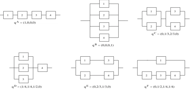
Example 2.1

Figure 2.1 presents the signatures of six coherent systems with m= 4 exchangeable components. Suppose that n = 4 components exchangeable with those in such a system were tested, leading to ordered failure times t1 < t2 < t3 < t4, which create

the partitionI1, . . . , I5 of the positive real-line. Table 2.1 presents the probabilities,

as given by Equation 1.15 and denoted by jPi = P(Tj:4 ∈ Ii) for j = 1, . . . ,4 and

i = 1, . . . ,5, together with the NPI lower and upper survival functions for Tj:4 as

given by Equations 1.16 and 1.17, respectively.

1 2 3 4 1 2 3 4 qA B q C q D q qE q = (0,0,0,1) = (1,0,0,0) 1 2 3 4 = (0,1/3,2/3,0) 1 2 3 4 = (1/4,1/4,1/2,0) 1 2 3 4 = (0,2/3,1/3,0) 1 2 3 4 = (0,1/2,1/4,1/4) F

Figure 2.1: Coherent systems with 4 exchangeable components

Table 2.2 presents the NPI lower and upper survival functions,STS(t) andSTS(t),

for the system failure timeTS, from Equations 2.1 and 2.2, for the systems presented

(27)

2.2. Predicting system failure time 18 j = 1 j = 2 j = 3 j= 4 i 1Pi ST1:4 ST1:4 2Pi ST2:4 ST2:4 3Pi ST3:4 ST3:4 4Pi ST4:4 ST4:4 1 0.500 0.500 1 0.214 0.786 1 0.071 0.929 1 0.014 0.986 1 2 0.286 0.214 0.500 0.286 0.500 0.786 0.171 0.757 0.929 0.057 0.929 0.986 3 0.143 0.071 0.214 0.257 0.243 0.500 0.257 0.500 0.757 0.143 0.786 0.929 4 0.057 0.014 0.071 0.171 0.071 0.243 0.286 0.214 0.500 0.286 0.500 0.786 5 0.014 0 0.014 0.071 0 0.071 0.214 0 0.214 0.500 0 0.500

Table 2.1: jPi, STj:4(t) and STj:4(t) fort ∈Ii, for n= 4 and m= 4

in Table 2.2 with the use of survival signature, as presented in that chapter. Table 2.2 illustrates that the upper survival function for the system failure time is always equal to one in the first interval and the corresponding lower survival function is less than one. Of course, these lower and upper survival functions decrease at each observed failure time of a component in the test. The lower survival function is zero after the largest observation while the upper survival functions always remains positive. Tables 2.1 and 2.2 show that the upper survival function in interval Ii is

equal to the lower survival function in intervalIi−1. This is a property that generally

holds for the lower and upper survival functions in this chapter, and which follows directly from Equations 1.16 and 1.17.

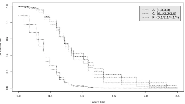
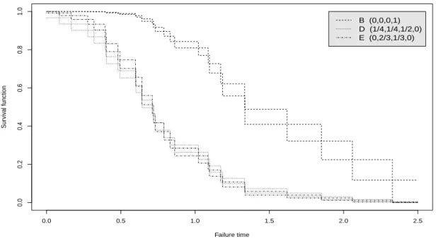
Figures 2.2 and 2.3 present the NPI lower and upper survival functions for the six systems in Figure 2.1 based onn = 30 observations of component failure times, simulated from the Weibull distribution with shape parameter 2 and scale parameter 1. The 30 ordered simulated component failure times are given in Table 2.3.

The signatures of systems C and F are not stochastically ordered (see Section 2.3), which leads to their NPI lower and upper survival functions crossing as is illustrated in Figure 2.2, and the same applies for systems D and E, shown in Figure 2.3. These lower and upper survival functions clearly indicate the differences in the system reliability for these six systems. However, one may wish to quantify the differences in reliability more precisely, a new approach that can be used for this will be presented in Section 2.3.

(28)

2.2. Predicting system failure time 19 q (1,0,0,0) (0,0,0,1) (0,1₃,2₃,0) i S_T_S STS STS STS STS STS 1 0.50 1 0.99 1 0.88 1 2 0.21 0.50 0.93 0.99 0.67 0.88 3 0.07 0.21 0.79 0.93 0.41 0.67 4 0.01 0.07 0.50 0.79 0.17 0.41 5 0 0.01 0 0.50 0 0.17 q (1₄,1₄,1₂,0) (0,2₃,1₃,0) (0,1₂,1₄,1₄) i S_T_S STS STS STS STS STS 1 0.79 1 0.83 1 0.87 1 2 0.56 0.79 0.59 0.83 0.67 0.87 3 0.33 0.56 0.33 0.59 0.44 0.67 4 0.13 0.33 0.12 0.33 0.21 0.44 5 0 0.13 0 0.12 0 0.21

Table 2.2: STS(t) and STS(t) for t∈Ii

0.086 0.167 0.277 0.319 0.394 0.400 0.402 0.481 0.494 0.599

0.601 0.642 0.642 0.712 0.720 0.732 0.790 0.832 0.863 1.023

1.088 1.097 1.172 1.185 1.334 1.336 1.620 1.851 2.060 2.329

(29)

2.2. Predicting system failure time 20 0.0 0.5 1.0 1.5 2.0 2.5 0.0 0.2 0.4 0.6 0.8 1.0 Failure time Sur viv al function A (1,0,0,0) C (0,1/3,2/3,0) F (0,1/2,1/4,1/4)

Figure 2.2: NPI lower and upper survival functions for system A, C and F (Ex. 2.1)

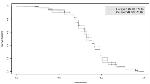
Example 2.2

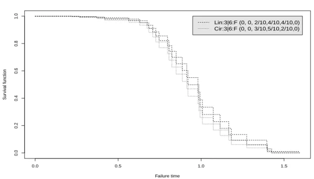
To further illustrate the NPI lower and upper survival functions for systems pre-sented in this chapter, consider linear and circular consecutive k-out-of-m:F sys-tems, which fail if and only if k or more linearly or circularly ordered components fail [44, 45, 55]. Table 2.4 gives n = 30 component failure times simulated from a Weibull distribution with shape parameter 3 and scale parameter 1. Figure 2.4 presents the NPI lower and upper survival functions, based on these data, for both a linear and circular consecutive 2-out-of-4:F system, for which the signatures are also given in the figure. The circular system fails for all neighbouring pairs of failing components for which the linear system fails, but in addition it also fails if only the first and last ordered components fail. This results in the circular system being less reliable than the linear system, as shown in Figure 2.4. Figure 2.5 presents similar NPI lower and upper survival functions for the linear and circular consecu-tive 3-out-of-6:F systems based on the same component failure data. These systems are clearly more reliable early on than the 2-out-of-4 systems. For all these four

(30)

2.2. Predicting system failure time 21 0.0 0.5 1.0 1.5 2.0 2.5 0.0 0.2 0.4 0.6 0.8 1.0 Failure time Sur viv al function B (0,0,0,1) D (1/4,1/4,1/2,0) E (0,2/3,1/3,0)

Figure 2.3: NPI lower and upper survival functions for system B, D and E (Ex. 2.1)

0.223 0.265 0.372 0.419 0.564 0.630 0.675 0.685 0.709 0.727

0.747 0.798 0.807 0.824 0.850 0.887 0.914 0.921 0.981 0.987

0.994 1.008 1.073 1.115 1.167 1.182 1.275 1.397 1.400 1.425

Table 2.4: 30 simulated component failure times for (Ex. 2.2)

systems considered, the lower survival function is zero beyond the largest observed component failure time, t = 1.425, reflecting that the data provide no evidence in favour of survival beyond this time, yet the corresponding upper survival functions are positive reflecting the fact that such survival cannot be deemed to be impos-sible on the basis of the 30 observations only. Figure 2.6 and 2.7 present the NPI lower and upper survival functions for linear consecutive 2-out-of-4 and 3-out-of-6 systems, and for circular consecutive 2-out-of-4 and 3-out-of-6, respectively.

(31)

2.3. Comparing failure times of two systems 22 0.0 0.5 1.0 1.5 0.0 0.2 0.4 0.6 0.8 1.0 Failure times Sur viv al functions Lin:2|4:F (0,1/2,1/2,0) Cir:2|4:F(0,2/3,1/3,0)

Figure 2.4: NPI lower and upper survival functions for the linear and circular con-secutive 2-out-of-4:F systems (Ex. 2.2)

2.3 Comparing failure times of two systems

System signatures provide a straightforward way to compare the reliability of two systems with m exchangeable components (so both systems having components of the same single type) if the signatures are stochastically ordered [61]. Let the sig-nature of system A be qa _{and of system} _B _be _qb_{, and let the failure times of these}

systems be Ta _and _Tb_{, respectively. If} Pm j=rq a j ≥ Pm j=rq b j for all r = 1, . . . , m

then P(Ta _{> t}₎ _≥ _P₍_Tb _{> t}_{) for all} _{t >} _{0. Such a comparison is even possible if}

the two systems do not have the same number of components, as one can always increase the length of a system signature in a way that does not affect the corre-sponding system’s failure time distribution [61], hence one can always make the two systems’ signatures of the same length. For example, the signatures (1

4, 1 4,

1

2,0) and

(0,1₅,3₅,1₅,0) do not have the same number of components. Using Equation 1.6 in Section 1.2, we find that the 5-component system with signature (2

10, 2 10, 3 10, 3 10,0)

(32)

2.3. Comparing failure times of two systems 23 0.0 0.5 1.0 1.5 0.0 0.2 0.4 0.6 0.8 1.0 Failure time Sur viv al function Lin:3|6:F (0, 0, 2/10,4/10,4/10,0) Cir:3|6:F (0, 0, 3/10,5/10,2/10,0)

Figure 2.5: NPI lower and upper survival functions for the linear and circular con-secutive 3-out-of-6:F systems (Ex. 2.2)

stochastically ordered with the signature (0,1 5,

3 5,

1

5,0) . However, many systems’

structures do not have corresponding signatures which are stochastically ordered. For example, the signatures (1

4, 1 4, 1 2,0) and (0, 2 3, 1

3,0) in the example in Section 2.2

are not stochastically ordered.

This section presents a different way to compare the random failure times Ta

and Tb _{of two systems} _A _and _B _{within the NPI framework, namely by considering}

the event that system B does not fail before system A, so Ta _≤ _Tb_{. This has the}

further advantage of being applicable to any two independent systems, so also to systems that each only have a single type of components but with the components of system A of a different type than those of system B. Subsection 2.3.1 presents NPI lower and upper probabilities for the eventTa _≤_Tb _{for two systems that share}

the same type of components, followed in Subsection 2.3.2 by such results for two systems with different types of components. Subsection 2.3.3 generalizes this by considering the event Ta_≤_Tb₊_δ _{for any real-valued constant} _δ_{, and how the NPI}

(33)

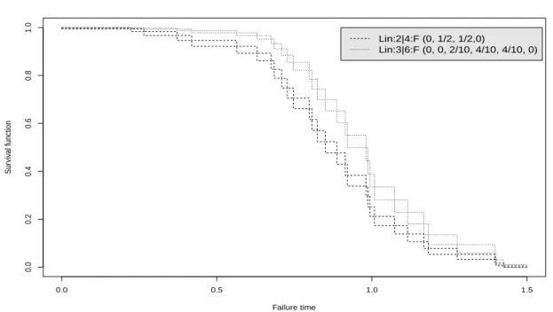
2.3. Comparing failure times of two systems 24 0.0 0.5 1.0 1.5 0.0 0.2 0.4 0.6 0.8 1.0 Failure time Sur viv al function Lin:2|4:F (0, 1/2, 1/2,0) Lin:3|6:F (0, 0, 2/10, 4/10, 4/10, 0)

Figure 2.6: NPI lower and upper survival functions for the linear consecutive 2-out-of-4:F and 3-out-of-6:F systems (Ex. 2.2)

lower and upper probabilities for this event behave as a function of δ. This enables a more detailed insight into the actual difference between the random lifetimes of the systems A and B.

2.3.1 Two systems with components of a single type

Consider two systems A and B with m components each and all their components assumed to be exchangeable, so both systems share components of a single type. Using the results presented in Section 2.2, it is easily seen that a similar result holds for the NPI lower and upper probabilities as for precise probabilities mentioned above, namely if Pm j=rq a j ≥ Pm j=rq b

j for all r= 1, . . . , m then P(Ta > t) ≥P(Tb > t) and P(Ta _{> t}₎ _≥ _P₍_Tb _{> t}_{) for all} _{t >} _{0. If the signatures} _qa _and _qb _are

not stochastically ordered, a different way to compare the systems’ failure times is needed, and indeed it is natural to consider the eventTa_≤_Tb_{. This does not require}

(34)

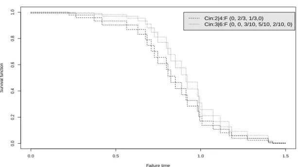
2.3. Comparing failure times of two systems 25 0.0 0.5 1.0 1.5 0.0 0.2 0.4 0.6 0.8 1.0 Failure time Sur viv al function Cin:2|4:F (0, 2/3, 1/3,0) Cin:3|6:F (0, 0, 3/10, 5/10, 2/10, 0)

Figure 2.7: NPI lower and upper survival functions for the circular consecutive 2-out-of-4:F and 3-out-of-6:F systems (Ex. 2.2)

components and systemB ofmb components, where the failure times of allma+mb

components are assumed to be exchangeable. Let the ordered random failure times of the components in systemA beTa

1:ma ≤T a

2:ma ≤. . .≤T a

ma:ma and let the ordered

random failure times of the components in systemBbeTb

1:mb ≤T b

2:mb ≤. . .≤T b mb:mb.

Using the signatureqa _and _qb _{of these systems, the following equality holds [61]}

P(Ta≤Tb) = ma X i=1 mb X j=1 qiaq b jP(T a i:ma ≤T b j:mb) (2.5)

This equality can be used directly in NPI without depending on observed failure times, due to the assumed exchangeability of the failure times of allma+mb

compo-nents. The probabilities in the sum on the right-hand side of (2.5) are precise-valued in NPI, so no use of lower and upper probabilities is required. These probabilities are P(Ta i:ma ≤T b j:mb) = ma+mb ma −1"j−1 X l=0 i−1 +l i−1 ma−i+mb−l ma−i # (2.6)

(35)

2.3. Comparing failure times of two systems 26

This follows by a straightforward counting argument, using the fact that exchange-ability of the ma +mb component lifetimes includes that their orderings are all

equally likely. This implies that the ma+mb ma

different orderings of the lifetimes of the ma components in system A and the mb components in system B, neglecting

the specific role played by each component in the system (note that this is taken into account by the signatures), are all equally likely. For the event Ta

i:ma ≤ T b j:mb

to occur, the number of components in system B failing before Ta

i:ma, so before the

failure time of thei-th failing component in system A, can be at most j−1. For a value of l ∈ {0,1, . . . , j−1}, the corresponding term in the sum in Equation (2.6) counts all equally likely orderings of the component failure times with precisely l

such failure times for components in system B occurring before Ta i:ma.

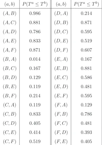
Table 2.5 presents the probabilities as given in Equations 2.5 and 2.6 for the events Ta _≤ _Tb _{for all combinations of two systems out of the six presented in}

Figure 2.1. Consider, for example, the systems D and E in Figure 2.1, which have signatures that are not stochastically ordered. Let their failure times be denoted by TD _and _TE_{, respectively, then} _P₍_TD _≤ _TE_{) = 0}_._{519 as shown in Table 2.5,}

which can be interpreted as indicating that these two systems are about equally reliable, with system E slightly more reliable than system D. While for systems A

andB in Figure 2.1, which have signatures that are stochastically ordered, we have

P(TA _≤ _TB_{) = 0}_._{986, which clear shows that system} _B _{is far more reliable than}

system A.

2.3.2 Two systems with different types of components

Let system A consist of ma exchangeable components, and system B of mb

ex-changeable components, with the components of the different systems being of dif-ferent types and their random failure times assumed to be fully independent, which means that any information about components of the type used in system A does not contain any information about components of the type used in system B, and vice versa. The ordered random failure times of the components in systemA and of those in systemB are denoted as in Subsection 2.3.1. Suppose that na components

(36)

2.3. Comparing failure times of two systems 27 (a, b) P(Ta≤Tb) (a, b) P(Ta≤Tb) (A, B) 0.986 (D, A) 0.214 (A, C) 0.881 (D, B) 0.871 (A, D) 0.786 (D, C) 0.595 (A, E) 0.833 (D, E) 0.519 (A, F) 0.871 (D, F) 0.607 (B, A) 0.014 (E, A) 0.167 (B, C) 0.167 (E, B) 0.881 (B, D) 0.129 (E, C) 0.586 (B, E) 0.119 (E, D) 0.481 (B, F) 0.214 (E, F) 0.595 (C, A) 0.119 (F, A) 0.129 (C, B) 0.833 (F, B) 0.786 (C, D) 0.405 (F, C) 0.481 (C, E) 0.414 (F, D) 0.393 (C, F) 0.519 (F, E) 0.405

Table 2.5: Pairwise comparisons of six systems from Figure 2.1

ta

1 < ta2 < . . . < tana, and similarly that ordered observed failure times of nb tested

components, exchangeable with those in system B, are tb

1 < tb2 < . . . < tbnb. Using

the signaturesqa _and _qb _{of these systems, a result similar to Equality 2.5 holds for}

the NPI lower probability for the event Ta_≤_Tb_{, namely}

P(Ta_≤_Tb_{) =} ma X i=1 mb X j=1 qa iqjbP(Tia:ma ≤T b j:mb) (2.7) where, as presented in [27] P(Tia:ma ≤T b j:mb) = na X l=1 P_la,i[P(Tjb:mb ≥t a l)] (2.8) with P_la,i = P(Ta i:ma ∈ (t a

l−1, tal)). The summation in (2.8) does not include a term

for l = n+ 1 because P(Tb

j:mb ≥ ∞) = 0. Let vl ∈ {1, . . . , nb + 1} be such that tb vl−1 < t a l < tbvl, then P(Tb j:mb ≥t a l) = nb+1 X v=vl+1 P(Tb j:mb ∈(t b v−1, tbv)) (2.9)

(37)

The justification of Equation 2.7 is similar to that of Equation 2.1 in Section 2.2, effectively the NPI lower probabilities for the eventsTa

i:ma ≤T b

j:mb, for i= 1, . . . , ma

and j = 1, . . . , mb, can all be attained simultaneously for the same underlying

configuration of observed and future failure times for components of type A (all future observations ‘at’ the right end-point of each interval) and the same underlying configuration of observed and future failure times for components of type B (all future observations ‘at’ the left end-point of each interval) [27]. The corresponding NPI upper probability for the event Ta _≤_Tb _{is derived and justified similarly, and}

is P(Ta≤Tb) = ma X i=1 mb X j=1 qiaq b jP(T a i:ma ≤T b j:mb) (2.10) where P(Tia:ma ≤T b j:mb) = na+1 X l=1 P_la,i[P(Tjb:mb ≥t a l−1)] (2.11) and P(Tjb:mb ≥t a l) = nb+1 X v=vl P(Tjb:mb ∈(t b v−1, t b v)) (2.12) Example 2.3

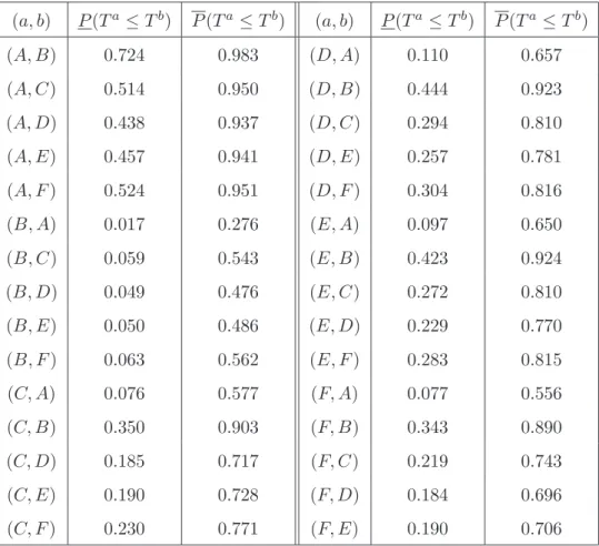
The pairwise comparison results presented in this section are illustrated using the six systems from Example 2.1, each with four exchangeable components but with the different systems considered having different types of components with independence of failure times assumed. Table 2.6 presents the NPI lower and upper probabilities for the events Ta _≤_Tb_{, as presented in Equations 2.7 and 2.10, for the failure times} Ta _and_Tb _{for all combinations of two systems out of the six presented in Figure 2.1.}

For all these 30 events, it is assumed that na = 3 components exchangeable with

those in the system with failure time Ta _and _n

b = 2 components exchangeable with

those in the system with failure time Tb _{have been tested and that the ordering}

of the test data is ta

1 < tb1 < ta2 < tb2 < ta3. Of course, the NPI lower and upper

probabilities in Table 2.6 show that systemA is the least reliable and systemB the most reliable of these systems. Notice that the comparisons of systems A, B, C, F

with either system D or E (whose signatures are not stochastically ordered) give very similar results, yet they all indicate that systemE is slightly more reliable than

(38)

2.3. Comparing failure times of two systems 29 (a, b) P(Ta≤Tb) P(Ta≤Tb) (a, b) P(Ta≤Tb) P(Ta≤Tb) (A, B) 0.724 0.983 (D, A) 0.110 0.657 (A, C) 0.514 0.950 (D, B) 0.444 0.923 (A, D) 0.438 0.937 (D, C) 0.294 0.810 (A, E) 0.457 0.941 (D, E) 0.257 0.781 (A, F) 0.524 0.951 (D, F) 0.304 0.816 (B, A) 0.017 0.276 (E, A) 0.097 0.650 (B, C) 0.059 0.543 (E, B) 0.423 0.924 (B, D) 0.049 0.476 (E, C) 0.272 0.810 (B, E) 0.050 0.486 (E, D) 0.229 0.770 (B, F) 0.063 0.562 (E, F) 0.283 0.815 (C, A) 0.076 0.577 (F, A) 0.077 0.556 (C, B) 0.350 0.903 (F, B) 0.343 0.890 (C, D) 0.185 0.717 (F, C) 0.219 0.743 (C, E) 0.190 0.728 (F, D) 0.184 0.696 (C, F) 0.230 0.771 (F, E) 0.190 0.706

Table 2.6: Pairwise comparisons of six systems from Figure 2.1 (Ex. 2.3)

system D, the same conclusion as drawn in Subsection 2.3.1. This is an attractive way to compare the random failure times of two systems, which takes both the system structures and the information from the test data directly into account and considers a natural event of interest. The NPI lower probability reflects the evidence in favour of the event Ta _≤ _Tb _{while the corresponding upper probability reflects}

the evidence in favour of the complementary eventTa _{> T}b_{. The difference between}

corresponding upper and lower probabilities, also called the ‘imprecision’, is due to the limited information available and the relatively weak modelling assumptions. In Table 2.6 the imprecision of most events is large, which is due to there being only 5 observations in total. If more test data are available, the imprecision typically becomes smaller, it would decrease to 0 if the numbers of test data in both groups go to infinity.

(39)

com-2.3. Comparing failure times of two systems 30 Data ordering P(TD ≤TE) P(TD ≤TE) td₁ < td₂ < t₃d< te₁ < te₂ 0.548 1 td 1 < td2 < te1 < td3 < te2 0.442 0.940 td₁ < td₂ < t₁e < te₂ < td₃ 0.371 0.869 td₁ < te₁ < t₂d< td₃ < te₂ 0.328 0.852 td₁ < te₁ < t₂d< te₂ < td₃ 0.257 0.781 te₁ < td₁ < t₂d< td₃ < te₂ 0.219 0.757 te₁ < td₁ < t₂d< te₂ < td₃ 0.149 0.686 td₁ < te₁ < t₂e< td₂ < td₃ 0.181 0.675 te₁ < td₁ < t₂e< td₂ < td₃ 0.072 0.580 te₁ < te₂ < t₁d< td₂ < td₃ 0 0.466

Table 2.7: Pairwise comparisons of systems D and E with nD = 3 and nE = 2

parison of systems D and E, considering the eventTD _≤_TE _with _n

D = 3 observed

failure times for components exchangeable with those in system D and nE = 2

ob-served failure times for components exchangeable with those in system E, and all possible orderings of these observed failure times. These lower and upper probabil-ities vary of course for the different data orderings, and also the imprecision varies. If the three tested components of type D all failed before the two components of type E, the data do not contain any evidence against the possibility that compo-nents of type D will always fail before components of type E, which is reflected in

P(TD _≤_TE_{) = 1 in this case. Similarly, the other extreme data ordering does not}

provide any evidence in favour of the possibility that components of type D will ever fail before components of typeE, as reflected byP(TD _≤_TE_{) = 0 for the final}

ordering in Table 2.7.

2.3.3 Difference between failure times of two systems

The method presented in Subsection 2.3.2 compares the random failure times of two systems by considering the event that one fails before the other, but it does not provide insight into the actual difference between these failure times. Therefore, the

(40)

approach of Subsection 2.3.2, using the same setting of two systems with different types of components, is now generalized by considering the event Ta _≤_Tb ₊_δ_{, for}

real-valuedδ. Of course, the setting of Subsection 2.3.1 can be similarly generalized. The following generalization of Equation 2.5,

P(Ta≤Tb+δ) = ma X i=1 mb X j=1 qiaq b jP(T a i:ma ≤T b j:mb +δ)

is proven in the same way as Equation 2.5, and is intuitively logical because adding the constant valueδ to the random lifetime of a system can be thought of as adding it to the lifetimes of all its components, doing so will not change the signature of the system. This immediately carries through to the NPI lower probability for this event, which is P(Ta≤Tb+δ) = ma X i=1 mb X j=1 qiaq b jP(T a i:ma ≤T b j:mb +δ) (2.13)

with the NPI lower probabilities in the sum on the right-hand side equal to

P(Ta i:ma ≤T b j:mb+δ) = na X l=1 P_la,i[P(Tb j:mb +δ ≥t a l)] (2.14)

Letvl,δ ∈ {1, . . . , nb+ 1} be such thattbvl,δ−1 < t a l −δ < tbvl,δ, then P(Tb j:mb+δ≥t a l) = nb+1 X v=vl,δ+1 P(Tb j:mb ∈(t b v−1, tbv)) (2.15)

The corresponding NPI upper probability for the event Ta_≤_Tb₊_δ _is

P(Ta_≤_Tb₊_δ_{) =} ma X i=1 mb X j=1 qa iqjbP(Tia:ma ≤T b j:mb +δ) (2.16) where P(Ta i:ma ≤T b j:mb+δ) = na+1 X l=1 P_la,i[P(Tb j:mb+δ ≥t a l−1)] (2.17) and P(Tjb:mb+δ≥t a l−1) = nb+1 X v=vl,δ P(Tjb:mb ∈(t b v−1, t b v)) (2.18)

Compared to the NPI lower and upper probabilities presented in Subsection 2.3.2, which correspond to those forδ = 0 here, calculation of these NPI lower and upper probabilities just follows from shifting themb test observations for components

(41)

exchangeable to those in system B by adding δ, or alternatively by subtracting δ

from each observation ta

l. For changing values of δ, these NPI lower and upper

probabilities only change ifδis large enough to change the ordering of thetb

1, . . . , tbnb

relative to the valuesta

1−δ, . . . , tana−δ, such a change of the ordering can happen for

at mostna×nb different values ofδ. Therefore,P(Ta≤Tb+δ) andP(Ta≤Tb+δ)

can have at most na ×nb + 1 different values (including the case δ = 0), and as

function of δ these lower and upper probabilities are step functions which change value at the same na×nb points, making their computation straightforward unless na×nb is very large.

Example 2.4

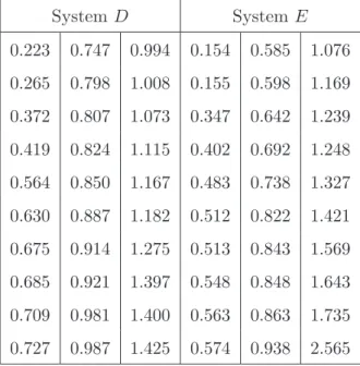
Systems D and E of Figure 2.1 have been of interest as their signatures are not stochastically ordered. Assume now that they have different types of components, and that nd = ne = 30 components exchangeable with those of each type in the

respective system have been tested, leading to the failure times in Table 2.8. These ordered failure times for system D were simulated from a Weibull distribution with shape parameter 3 and scale parameter 1, and for system E from a Weibull distri-bution with shape parameter 2 and scale parameter 1.

System D SystemE 0.223 0.747 0.994 0.154 0.585 1.076 0.265 0.798 1.008 0.155 0.598 1.169 0.372 0.807 1.073 0.347 0.642 1.239 0.419 0.824 1.115 0.402 0.692 1.248 0.564 0.850 1.167 0.483 0.738 1.327 0.630 0.887 1.182 0.512 0.822 1.421 0.675 0.914 1.275 0.513 0.843 1.569 0.685 0.921 1.397 0.548 0.848 1.643 0.709 0.981 1.400 0.563 0.863 1.735 0.727 0.987 1.425 0.574 0.938 2.565

(42)

Figure 2.8 presents the NPI lower and upper probabilities for the event Td _≤ Te ₊ _δ _{as function of} _δ_{. In the top-left figure, Figure 2.8.1, these functions are}

given for the data in Table 2.8. For these data, these functions remain constant for values of δ less than −2.342 or greater than 1.271, as in these cases the two data sets are completely non-overlapping, which shows in the fact that the NPI lower probability for this event is equal to zero for δ < −2.342 and the NPI upper probability for this event is equal to one for δ > 1.271. Actually, the changes in these NPI lower and upper probabilities atδequal to−2.342 or 1.271 are very small and not well visible in Figure 2.8.1. The same is true at other values of δ close to these minimal and maximal ones at which the NPI lower and upper probabilities change. At δ = −2.342, the NPI lower probability Td _≤ _Te₊_δ _{increases from 0}

to 0.00013 and the NPI upper probability increases from 0.03630 to 0.03656, while atδ = 1.271 the lower probability increases from 0.98702 to 0.98717 and the upper probability increases from 0.99996 to 1.

The three further figures included in Figure 2.8 show the effect of substantial changes to the actual observations, that is changes that actually change the order of the observations, and hence they show how the NPI lower and upper probabilities for the event Td _≤ _Te ₊_δ _{adapt to changes in the component test data. First,}

the largest observed failure time for system D, 1.425, is replaced by 3.425, which makes it the largest observed value in both sets of data. The resulting NPI lower and upper probabilities for the event Td _≤ _Te₊_δ _{as functions of} _δ _{are presented}

in Figure 2.8.2, but the effect on the figures is not well visible when compared to the original situation in Figure 2.8.1. Figures 2.8.3 and 2.8.4 show the NPI lower and upper probabilities with the largest 4 and 10, respectively, values for System

D, as given in Table 2.8, changed by adding 2 to the original data values, which implies that these all become larger than the largest observation for SystemE. Now the effect is clear in both figures, and of course substantially stronger in case 10 observations have been changed. Figure 2.9 presents the same functions of Figures 2.8.1 and 2.8.4, so for the original data and with 10 values changed, on a larger scale to see the differences more clearly. While the differences for the larger values of δ

(43)

−4

−2

0

2

4

0.0 0.4 0.8

1

−4

−2

0

2

4

0.0 0.4 0.8

2

−4

−2

0

2

4

0.0 0.4 0.8

3

−4

−2

0

2

4

0.0 0.4 0.8

4

(44)

2.4. Concluding remarks 35 −4 −2 0 2 4 0.0 0.2 0.4 0.6 0.8 1.0

Figure 2.9: Difference of failure times of two systems (Figures 2.8.1 and 2.8.4)

close to 0 and even for negative values ofδ.

2.4 Concluding remarks

In this chapter we have introduced the use of signatures in the study of system failure times with lower and upper probabilities. There are many related research challenges, for example a slightly more challenging topic is simultaneous comparison of more than two systems’ failure times. The NPI lower and upper probabilities for pairwise comparisons, as presented in Section 2.3, cannot be combined directly into such quantifications for multiple comparisons. For example, it may be of interest to consider the event that a particular one of the systems considered is the most reliable in the sense of its random failure time being the largest of all systems’ failure times, so it is of interest to generalize the method presented in Section 2.3 to derive NPI lower and upper probabilities for such events. This can be done in NPI along

Nonparametric Predictive Inference for System Failure Time

Durham E-Theses

Nonparametric Predictive Inference for System Failure

Time

Nonparametric Predictive Inference for

System Failure Time

Abdullah H. Al-nefaiee

A thesis presented for the degree of

Doctor of Philosophy

Department of Mathematical Sciences

University of Durham

England

2014

Dedicated to

my parents

Nonparametric predictive inference for

system failure times

Abdullah H. Al-nefaiee

Submitted for the degree of Doctor of Philosophy

2014

Abstract

Declaration

Acknowledgements

Contents

Chapter 1

Introduction

1.1

Overview

1.2

System signatures

1.3

Nonparametric predictive inference (NPI)

1.4

NPI for order statistics

1.5

NPI for Bernoulli quantities

1.6

Outline of thesis

Chapter 2

Failure time of a system consisting

of exchangeable components

2.1

Introduction

2.2

Predicting system failure time

2.3

Comparing failure times of two systems

2.3.1

Two systems with components of a single type

2.3.2

Two systems with different types of components

2.3.3

Difference between failure times of two systems

−4

−2

0

2

4

1

−4

−2

0

2

4

2

−4

−2

0

2

4

3

−4

−2

0

2

4

4

2.4

Concluding remarks