E¢ cient M-estimators with auxiliary information
Francesco Bravo
yUniversity of York
First version September 2008
Revised September 2009
Abstract
This paper introduces a new class of M-estimators based on generalised em-pirical likelihood (GEL) estimation with some auxiliary information available in the sample. The resulting class of estimators is e¢ cient in the sense that it achieves the same asymptotic lower bound as that of the e¢ cient generalised method of moment (GMM) estimator with the same auxiliary information. The paper also shows that in case of smooth estimating equations the proposed es-timators enjoy a small second order bias property compared to both e¢ cient GMM and full GEL estimators. Analytical formulae to obtain bias corrected estimators are also provided. Simulations show that with correctly speci…ed auxiliary information the proposed estimators and in particular those based on empirical likelihood outperform standard M and e¢ cient GMM estimators both in terms of …nite sample bias and e¢ ciency. On the other hand with moder-ately misspeci…ed auxiliary information estimators based on the nonparametric tilting method are typically charactersed by the best …nite sample properties.
Keywords and Phrases: Asymptotic e¢ ciency, Generalised empirical likelihood, Generalised method of moments, Second order bias.
This paper is dedicated to Jemima.
yI would like to thank Peter Phillips for helpful comments. Address correspondence to: Francesco Bravo, Department of Economics and Related Studies, University of York, York, Y010 5DD, United Kingdom. email:[email protected]
1
Introduction
Since the seminal paper of Huber (1964) M-estimators, which are generalisations of the usual maximum likelihood estimators, have played an important role in statistical theory; see for example Van der Vaart (1998, Chapter 5). In this paper we introduce a new class of M-estimators, which is motivated by the fact that in many situations of practical interest we may have some auxiliary information about the otherwise un-known distributionF of the sample. For example we might know the probability that the observed data belong to a certain part of the sample space, or thatF has given known moments (joint or marginal), or that is symmetric around a certain constant. This information is often available from auxiliary data such as national statistics or the census. Alternatively the auxiliary information can be a direct by-product of a given theoretical model. In these situations we might expect that incorporating such information into the estimation process can reduce the bias and increase the e¢ ciency of the parameter estimates. For example Imbens and Lancaster (1994) and Hellerstein and Imbens (1999) use auxiliary information within a generalised method of moments (GMM) regression framework, whereas Handcock, Houvilainen and Rendall (2000) combine sample and auxiliary information within generalised linear models. Imbens and Lancaster (1994) report substantial e¢ ciency gains in the parameter estimates by incorporating marginal moments from Census data.
The main objective of this paper is to propose a simple two-step method to in-corporate auxiliary information into an M-estimation process. The method is based on the generalised empirical likelihood (GEL) estimator developed by Smith (1997) (see also Newey and Smith (2004) and references therein). To be speci…c in the …rst step GEL is used to obtain an estimator of F that is consistent with the auxiliary information available in the sample. This estimator is typically more e¢ cient than the empirical distribution function normally used in nonparametric settings and puts unequal weight on each of the observations. In the second step the parameters of in-terest are then estimated using the same estimating equations that would have been used if the auxiliary information was not available, but with the contribution of each observation multiplied by its corresponding weight. This weighted estimation proce-dure de…nes a new class of M-estimators (WM-estimators henceforth) that typically will be more e¢ cient than usual M-estimators. Intuitively, the latter are based on an estimator of F - the empirical distribution function- that is not e¢ cient in presence of auxiliary information, whereas the former are based on an estimator - the GEL
distribution function- that by construction makes e¤ective use of this information. The two-step estimation method of this paper is a generalisation of that proposed by Zhang (1995) and Hellerstein and Imbens (1999) - see also Owen (2001, Chapter 3.11). These authors use empirical likelihood to obtain the weights to be used in the estimation. Empirical likelihood however is only one of the possible estimators that can be used; one could in fact use Owen’s (1991) euclidean likelihood. Another possibility is to use Efron’s (1981) nonparametric tilting, or the more general empirical Cressie-Read statistic as de…ned by Baggerly (1998). These methods di¤er from each other either in terms of computational complexity or in terms of enjoying desirable statistical properties. For example, Brown and Chen (1998) used Euclidean likelihood because of its computational simplicity, whereas Imbens, Spady and Johnson (1998) used nonparametric tilting because of its robustness and numerical stability. They also typically di¤er in terms of …nite sample properties. On the other hand all of these methods share a common structure of being members of the general class of GEL. Thus GEL provides a general and convenient unifying method to obtain a large class weighted estimators.
The two-step estimation method of this paper can be related to other methods including GMM, full (or one-step) GEL (Parente and Smith, 2005), and parametric likelihood estimation. All of these methods include the auxiliary information directly into the estimation process and produce M-estimators that are asymptotically equiv-alent to those obtained in this paper (i.e. they have the same asymptotic variance). However the proposed two-step procedure seems to be preferrable to these alterna-tives for two reasons: First it is computationally simpler because it involves two separate optimisation problems, which are typically easier to solve numerically espe-cially for highly nonlinear models. Second in the case of smooth estimating equations the resulting WM-estimators enjoy a small second order bias property, that is the bi-ases have less components than those based on both GMM and full GEL estimators, which in fact tend to be more biased in …nite samples - see the simulations presented in Section 4 for some evidence. This interesting property is a direct consequence of the di¤erent way the auxiliary information is incorporated into the estimation process (i.e. directly in the case of GMM and GEL, indirectly in the case of the two-step estimation), and of the fact that the auxiliary information does not contain nuisance parameters. Indeed with nuisance parameters the property would typically not hold. Perhaps more importantly the resulting WM-estimators would not be asymptotically equivalent to those based on either GMM or full GEL estimation and would be
typi-cally ine¢ cient.
In this paper we make several contributions: …rst we establish consistency and asymptotic normality of the WM-estimators based on GEL estimation of auxiliary information. We show that they are e¢ cient in the sense that they have the same asymptotic variance as that of the e¢ cient GMM estimator with the same auxiliary information. Second we show how GEL can be used to consistently estimate the asymptotic variances of the WM-estimators. Third we consider the case where the auxiliary information is misspeci…ed (i.e. it is inaccurate), and investigate the asymp-totic properties of the WM-estimators under local misspeci…cation. Fourth we obtain expressions for the second order biases of the WM-estimators and compare them with those of GMM and GEL estimators. These expressions can be used to obtain analyt-ical bias corrected versions of all of these estimators. Finally we illustrate the results with two empirically relevant examples: an instrumental variable quantile regression model and a binary dependent variable regression model. for these two models we use simulations to assess and compare the …nite sample performances of the WM, stan-dard M and e¢ cient GMM estimators with both correct and moderately misspeci…ed auxiliary information.
The results of this paper are quite general and can be used in practice to improve the e¢ ciency of a large number of M-estimators de…ned both by smooth and non-smooth estimating equations, including the robust estimators of Huber (1973), the regression quantiles of Koenker and Basset (1978) and the trimmed least squares of Powell (1986) among others.
The rest of the paper is structured as follows: next section describes brie‡y GEL estimation. Section 3 contains the main results, whereas Section 4 illustrates the results of this paper with two examples, and reports the results of the simulations. Section 5 contains some concluding remarks. An appendix contains all the proofs.
The following notation is used throughout the paper: “a:s:” stands for almost surely,a:s:!,!p ,!d denote convergence almost surely, in probability and in distribution, respectively, and k k denotes the Euclidean norm. Finally “ ” denotes transpose, while “0” denotes derivative.
2
GEL estimation with auxiliary information
We begin this section with a simple example which motivates the two-step estimation procedure proposed in this paper.
Example 1.(Hellerstein and Imbens, 1999) Let xdenote a random variable with unknown distribution F, and suppose we want to estimate the population mean . Without any auxiliary information about F the sample mean x = Pni=1xi=n is the
e¢ cient estimator for . Consider now estimation of knowing thatPr (x >0) =p. While x is still consistent, it is no longer e¢ cient. The e¢ cient estimator for is in fact the weighted averagexp =px1+(1 p)x0wherex1 =
Pn i=1xiIfxi >0g= P Ifxi >0g and x0 = Pn i=1xiIfxi 0g= P
Ifxi 0g. This estimator can also be written as
xp = Pn i=1wixi=nwherewi = (p=p) Ifxi>0g [(1 p)=(1 p)]Ifxi 0g andp=PIfxi >0g=n
and note that the asymptotic normalised variance ofxp isE[V (xjIfxi >0g)]so that
n[V (x) V (xp)] = V (x) E[V (xjIfxi >0g)] =V [E(xjIfxi >0g)]>0
asn ! 1.
Example 1 clearly shows that incorporating weights obtained from available aux-iliary information into an estimation process can increase its precision. It is precisely this type of weighted estimation that we are going to focus on in this paper.
Let fxig n
i=1 be a random sample from an unknown distribution F with support
X <: Suppose that there exists some auxiliary information about F that can be expressed as a “moment function”
Z
g(x)dF (x) = E[g(x)] = 0; (1) whereg(x) is an<q-valued vector of functionally independent measurable functions.
To describe how GEL estimation can be used in (1), let (v) denote a function of a scalar v that is concave on its domain, an open interval V containing 0. Let
Vn :=f : g(xi)2 V, i= 1; :::; ng and de…ne the GEL class of functions
Gn( ) = n
X
i=1
( g(xi))=n
where is an <q-valued vector of unknown parameters.
Gn( ) includes as special
cases empirical likelihood (EL) with (v) = log (1 v) and V = ( 1;1), (NT) nonparametric tilting with (v) = exp (v), Euclidean likelihood (EU) with (v) = (1 +v)2=2 and the family of empirical Cressie-Read statistics (ECR) with (v) = (1 +v)(1+ )= =(1 + ) where 2 < is a user-speci…ed constant. In the rest of the paper we impose the following normalisation on (v): let j(v) = dj (v)=dvj and
j := j(0) (j = 1;2; :::); we normalise so that 1 = 2 = 1.1
1As long as
Let b:= arg max 2VnGn( ); the estimated weights b wi = 1 b g(xi) = n X j=1 1 b g(xj) ; (2)
sum to one by construction, satisfy the sample moment condition Pni=1wbig(xi) = 0
when the …rst order conditions for b hold (by the strong law of large numbers), and are positive when b g(xi) is uniformly small in i. Thus they can be interpreted as
implied probabilities which incorporate the auxiliary information as de…ned in (1). Given wbi the GEL distribution function estimator of F is de…ned as
b Fw(x) = n X i=1 b wiIfxi xg:
The following theorem summarises the basic asymptotic properties of b and Fbw(x);
letE[g(x)g(x) ] := :
Theorem 1 Assume that Ekg(x)k < 1 for some > 2, is positive de…nite,
and (v) is twice continuously di¤erentiable in a neighbourhood of 0. Then b :=
arg max 2VnGn( ) exists a:s: and
n1=2b!d N 0; 1 : (3) Moreover n1=2 Fbw(x) F (x) d !N(0; VFw(x)); (4) where VFw(x) = F(x) (1 F(x)) E[g(xi)Ifxi xg] 1E[g(x i)Ifxi xg]:
Equation (4) clearly shows that in presence of (1) the estimator Fbw(x) based on
the implied probabilities(2) is more e¢ cient than the empirical distribution function
b
Fn(x) =
Pn
i=1Ifxi xg=n:It is precisely this e¢ ciency property ofFbw(x)that will
be used in the rest of the paper to obtain more e¢ cient M-estimators.
3
Main results
Let (x; ) :<d
! <k denote a known vector of functions up to
0 such that
( ) :=E (x; ) (5)
be imposed by replacing (v)by 2= 21 [( 1= 2)v]:It is satis…ed by EL, NT and ECR among others.
and
( ) = 0at = 0
where 0 2 intf g, and <k is the parameter space. In a fully nonparametric
setting, an M-estimatorbof 0 solves approximately
n b inf 2 k n( )k+oa:s:(1); (6) where n( ) := Z (x; )dFbn(x) = n X i=1 (xi; )=n
is the sample analogue of (5). Note that in the most recent statistical literature an estimator that solves (6) is also referred as Z estimator (see Van der Vaart (1998)). Note also that if (x; ) is smooth(6) simpli…es to the more familiar
b:= arg min
2 k n( )k:
3.1
Correctly speci…ed auxiliary information
Suppose that there exists auxiliary information aboutF available in the moment form given in(1). In order to include such information into the estimation process, let
w( ) := Z (x; )dFbw(x) = n X i=1 b wi (xi; )
denote the weighted sample analogue of (5) where the implied probabilities wbi are
as in (2). Then we de…ne the class of WM-estimatorsbw as
w bw inf
2 k w( )k+oa:s(1): (7)
The following theorem establishes the strong consistency ofbw:
Theorem 2 Suppose that (I) the parameter space is a compact set, (II) for all
>0 infk 0k> k ( )k "( )>0, (III) sup 2 k n( ) ( )k=oa:s:(1). Then,
under the assumptions of Theorem 1 bw
a:s:
! 0:
The conditions of Theorem 2 are fairly standard in both the statistical and econo-metric literature on nonlinear models estimation. Su¢ cient conditions for the uni-form convergence (III) to hold are: (I), (x; ) continuous at each 2 a:s:, and
Esup 2 k (x; )k <1. Note however that the (III) is often stronger than needed for consistency of the estimator. The following theorem replaces uniformity with monotonicity as in Huber (1964). Assume that (x; ) :< ! < and <.
Theorem 3 Suppose that (I) the parameter space is an open interval, (II) for all
> 0 infj 0j> j ( )j "( )> 0, (III) there exists a neighbourhood N0 of 0 such
that EsupN0j (x; )j < 1, (IV) (x; ) is continuous and monotone in . Then,
under the assumptions of Theorem 1 bw
a:s:
! 0:
The following theorem establishes the asymptotic normality for the GEL-based WM-estimatorbw satisfying(7) without assuming smoothness of (x; ):
Theorem 4 Suppose that n1=2 b
w 0 =Op(1), and (I) there exists a …nite
non-singular matrix such that limk 0k!0k ( ) ( 0)k = o(k 0k), (II) for
all positive n ! 0 supk 0k nk n( ) ( ) n( 0)k = op n
1=2 (III) (a)
(x; ) is continuous at 0 a:s. (b) there exists a neighbourhood N0 of 0 such that
EsupN0k (x; )g(x)k < 1 (IV) n1=2
n(x; 0)
d
! N(0; V ( 0)), (V) 0 2 intf g.
Then under the assumptions of Theorem 1
n1=2 bw 0 d !N(0; g( 0)); where g( 0) = 1 V ( 0) E[ (x; 0)g(x) ] 1E[ (x; 0)g(x) ] ( ) 1 :
As with Theorem 2, the conditions of Theorem 4 are fairly standard. Suf-…cient conditions for the n1=2-consistency condition to hold are that b
w satis…es w bw inf 2 k w( )k+op n 1=2 together with the local di¤erentiability
of ( ) (I), the local stochastic equicontinuity (II) and a central limit theorem (IV). The following theorem establishes the asymptotic normality for the WM-estimator
bw using conditions similar to those used by Huber (1964, Lemma 4).
Theorem 5 Suppose that bw satis…es (7), bw p
! 0, and (I) ( ) is di¤erentiable
at = 0 with 0( 0) 6= 0 (II) (x; ) is monotone in , (III) E 2(x; ) and
E[ (x; )g(x)] are continuous at = 0, (IV) there exists a neighbourhood N0 of 0
such that EsupN0 2(x; ) <1 and EsupN0[j (x; )j kg(x)k]<1 . Then, under
the assumptions of Theorem 1,
n1=2 bw 0 d !N 0; 20g( 0) ; where 2 0g( 0) = E 2(x; 0) E[ (x; 0)g(x) ] 1E[ (x; 0)g(x)] = 0( 0)2: (8)
The following theorem establishes the asymptotic normality for the WM-estimator
bw assuming that (x; ) is di¤erentiable; let 0(x; 0) =@ (x; )=@ j = 0. Theorem 6 Suppose thatbw satis…es w bw = inf 2 k w( )k,bw
p
! 0, and (I)
(x; ) is continuously di¤erentiable in a neighbourhood N0 of 0, (II) E[ 0(x; )]is
continuous and nonsingular at 0,E k (x; 0)k kg(x)k
2
<1, there exists a
neigh-bourhood N0 of 0 such that EsupN0[k
0(x; )
k kg(x)k] <1 (III) n1=2 n(x; 0)
d
!
N(0; V ( 0)), (IV) 0 2intf g Then, under the assumptions of Theorem 1
n1=2 bw 0 d !N 0; 0g( 0) ; where 0g( 0) = [E 0(x; 0)] 1 V ( 0) E[ (x; 0)g(x) ] 1E[ (x; 0)g(x) ] [E 0(x; 0) ] 1 (9) Theorems 4-6 show that in presence of auxiliary information (1) on F, the as-ymptotic variances of the weighted estimatorsbw are always smaller than or equal to
the asymptotic variances of the corresponding WM-estimators(6), which are, respec-tively, 1V ( 0) ( ) 1,E 2(x; 0)= 0( 0)2and[E 0(x; 0)] 1 V ( 0) [E 0(x; 0) ] 1 :
The reduction in the asymptotic variance will depend on the relevance of the auxil-iary information: the larger the correlation between (x; )andg(x)the greater the gain in precision.
Remark 1 Calculations show that g( 0) corresponds to the asymptotic
vari-ance of the e¢ cient GMM estimator is given by
I( 0) 1 = n [ ;0] [Eh(x; 0)h(x; 0) ] 1 [ ;0] o 1 ;
where h(x; ) = [ (x; ) ; g(x) ] . Thus the estimators of this paper are e¢ cient in the class of GMM estimators de…ned as
Wn1=2Hn bGM M inf 2 W 1=2 n n X i=1 h(xi; )=n +oa:s(1); (10)
where Wn is a (possibly random) positive semi-de…nite weighting matrix. Moreover
if we assume that (x; ) is di¤erentiable, it is well-known (Chamberlain, 1987) that
I( 0) 1 is the lower bound for any n1=2 consistent regular estimator of 0 under
the sense that they achieve the (semiparametric) information lower bound for models de…ned by E[h(x; 0)] = 0:
We now consider the problem of estimating g( 0). We propose to use the
following GEL-based estimator
b g bw =bwb1 ( b Vwb bw n X i=1 b wi h xi;bw g(xi) i b 1 b w (11) n X i=1 b wi h xi;bw g(xi) i ) bw 1; where Vbwb bw = Pn i=1wbi xi;bw xi;bw , bwb = Pn i=1wbig(xi)g(xi) , and bwb is an estimator of whose form depends on the smoothness of (x; ). In the smooth case contains ordinary derivatives which can be easily estimated (see Remark 2 below). In the nonsmooth case a general strategy to estimate is to use numerical derivatives, that is bwb jl = n X i=1 b wi h j xi;bw+bnel j xi;bw i =bn j; l = 1; :::; k
where bn ! 0 at an appropriate rate as n ! 1, and el is lth unit vector. The
following theorem establishes the weak consistency of b g bw .
Theorem 7 Suppose that bn ! 0, b2nn ! 1, there exists a neighbourhood N0 of 0
such that EsupN0 k (x; )k2 < 1, and that the conditions of Theorems 1, 2, and
4 hold. Then
b g bw p
! g( 0):
Remark 2 A practical problem for the computation of (11) is the choice of the size ofbnused to form the numerical derivatives. This is in general a di¢ cult problem,
similar in fact to the choice of bandwidth in nonparametric density estimation. In speci…c cases it is possible to construct estimators that do not involve numerical di¤erentiation. For example if is proportional to (or features) the (unknown) density
f(x; ) an alternative estimator for can often be based on kernel methods - see Example 2 below. Another case is when (x; ) is di¤erentiable a:s: with derivative that is continuous in a:s: and dominated by an integrable function. On the other hand in the smooth case bwb =
Pn
i=1 0i bw wbi, and it is easy to show that (11) is
We …nally consider one-step WM-estimators and show that they have the same asymptotic distribution as that of the “fully iterated”WM-estimatorbw of Theorem
5. Consider solving w bw = 0 using the Newton’s algorithm starting with bw.
The full GEL-based WM-estimator is de…ned as
b1w =bw " n X i=1 b wi 0 xi;bw # 1 n X i=1 b wi xi;bw :
Theorem 8 Suppose that the conditions of Theorem 5 hold, and thatn1=2 bw 0 =
Op(1):Then,
n1=2 b1w 0
d
!N 0; 0g( 0) ;
where 0g( 0) is as in (9).
Remark 3All of the results of this section can be generalised by introducing a se-quence of nonsingular random matricesMn(xi; )and consideringkMw(xi; ) w( )k,
as for example in the classical method of minimum 2. As long assup
2 kMn(xi; )k
is bounded and converges to a nonsigular asymptotic matrix M( 0)it is not di¢ cult
to show that the resulting WM-estimator is consistent and asymptotically normal with covariance
g( 0) = 1fM( 0)V ( 0)M( 0) E[M( 0) (x; 0)g(x) ] 1E[M(
0) (x; 0)g(x) ] ( ) 1:
3.2
Misspeci…ed auxiliary information
Thus far we assumed that the auxiliary information (1) is correctly speci…ed (i.e. it is accurate, or at least accurate with a negligible sampling error). There are however empirically relevant situations in which this might not be necessarily the case. There-fore it is of interest to investigate what are the consequences of using misspeci…ed (i.e. inaccurate) information on the estimation procedure of this paper. In this section we consider two types of misspeci…cation: a global and a local one. The former can be parameterised as
E[g(x)] = 6= 0: (12) An example of (12)is the situation where the auxiliary information is obtained from a sample that is not compatible with the one used in the estimation, in the sense that the two samples are drawn from a di¤erent population. Another example is
the situation where there is a measurement error in the auxiliary information. In both cases the function g(x) needs not have zero expectation when the expectation is taken over the sample population.
Remark 4 The proofs of Theorems 1 and 2 show that when (12) is true the parameter estimator bw is in general inconsistent and n1=2 n bw diverges. This
follows because the almost sure limit of the estimatorbis not zero, implying that the GEL weights (2) e¤ectively introduce an almost sure non zero term which typically a¤ects the asymptotics of the WM-estimator.
We can test directly whether E[g(x)] = 0 using, for example, a GEL or a Wald test statistic, that is
Gn = 2 n X i=1 h b g(xi) (0) i ; (13) Wn = ng n X i=1 g(xi)g(xi) =n ! 1 g
where g =Pni=1g(xi)=n. The asymptotic distributions of Gn and Wn are 2p: If the
p-values of (13) are reasonably high we should be fairly con…dent that the auxiliary information available is accurate enough that possibly only a small error is intro-duced into the M-estimation via the constraintPni=1wbig(xi) = 0. On the other hand
if the p-values are relatively low then the auxiliary information might be moderately misspeci…ed. This situation is empirically relevant, because it is likely that typical sources of auxiliary information such as the Census contain some form of mild mis-speci…cation (due for example to the presence of measurement error). In Section 4 we use simulations to investigate the …nite sample e¤ects of using this type of misspeci…ed auxiliary information in the weighted estimation.
The second type of misspeci…cation is a local one, that is
E[g(x)] = =n1=2: (14) This is a situation in between the assumption of knowledge of correctly speci…ed aux-iliary information and that of a globally misspeci…ed information, because it captures the case where the auxiliary information is misspeci…ed for any …nite n but the size of the variation isO n 1=2 so that it vanishes asymptotically.
1
n1=2b!d N 1 ; 1 ; n1=2 Fbw(x) F(x)
d
!N( ; VFw(x));
where = E[g(xi)Ifxi xg] 1 and VFw(x) is the asymptotic variance as
de-…ned in (4):
Theorem 10 Suppose that (14) holds. Then under the same assumptions of
Theo-rems 2 or 3 bw
a:s:
! 0.
Theorem 11 Suppose that (14) holds. Then under the same assumptions of Theo-rems 4-6
n1=2 bw 0
d
!N( ( 0); Vg( 0)); (15)
where ( 0) = 1E[ (x; 0)g(x) ] 1 with Vg( 0) = g( 0) in the case of
Theorem 4, ( 0) = E[ (x; 0)g(x) ] 1 =[ 0(x; 0)]
2
with Vg( 0) = 2 0g( 0)
in the case of Theorem 5, and ( 0) = [E 0(x; 0)]
1
E[ (x; 0)g(x) ] 1 with
Vg( 0) = 0g( 0) in the case of Theorem 6.
Remark 5 Calculations show that the asymptotic distribution of the e¢ cient GMM estimator (and hence that of the full GEL estimator) under the local mis-speci…cation (14) is(15). Thus the WM estimators of this paper are asymptotically equivalent to both GMM and GEL estimators under local misspeci…cation.
The following …gure shows the e¤ect of local misspeci…cation in terms of …nite sample bias of a simple weighted least squares estimator for the regression parame-ters of yi = 0xi +"i where 0 = [0;0:5] , xi = [1; x1i] , and [x1i; "i] N(0; I).
The auxiliary information is parameterised as E(y) = =n1=2 where = 30, and is
estimated by empirical likelihood. Note that values closer to the origin correspond to bigger sample sizes.
Figure 1 approximately here
3.3
Higher order comparisons
The previous two sections showed that under both correct and locally misspeci…ed auxiliary information WM, GMM and (hence) (full) GEL estimators are asymptot-ically equivalent. In this section we assume that (x; ) is smooth and investigate the higher order asymptotic properties of the WM-estimators.
The following theorem gives a third order stochastic expansion for WM-estimators under regularity conditions similar to those used for example by Newey and Smith (2004); let @k( ) =@k( )= j1::::@ jk.
Theorem 12 Suppose that bw satis…es the conditions of Theorem 6, and that (I)
(x; )is four times continuously di¤erentiable in a neighbourhoodN0 of 0, (II) there
exists a neighbourhoodN0 of 0 such that fork = 1; :::;4(a)Esup 2N0 @
k (x; ) < 1, (b) Esup 2N0h @k (x; ) kg(x)kki, (c) Eh @k 1 (x; 0) kg(x)kk i < 1 (d)
Ekg(x)kk < 1, (III) (v) is four times continuously di¤erentiable in a
neighbour-hood of 0. Then
n1=2 bw 0 =Q1+Q2 +Q3+Op n 3=2 ; (16)
where Q1
d
! N 0; 0g( 0) , 0g( 0) is as in (9), Q2 and Q3 are, respectively, an
Op n 1=2 quadratic and Op(n 1)cubic polynomial in (x; 0)andg(x)whose exact
expressions are given in (32) and (33) in the Appendix.
The following corollary gives an explicit expression for the second order bias of
n1=2 b
w 0 . Lettr( ) denote the trace operator, (j) denote the jth (j = 1; :::; k)
component of , and let g (x) = 1=2g(x) denote the standardised auxiliary
infor-mation.
Corollary 13 Under the assumptions of Theorem 12 the second order bias for
n1=2 bw 0 is given by Biashn1=2 bw 0 i = [Bw1 + (1 + 3=2)Bw2]=n 1=2; (17) where Bw1 = [E( 0(x; 0))] 1n Eh 0(x; 0) (E[ 0(x; 0)]) 1 (x; 0) i E " k X j=1 @ 0(x; 0)=@ (j) # [E( 0(x; 0))] 1 V ( 0) [E( 0(x; 0))] 1 =2 ) [E( 0(x; 0))] 1 Eh 0(x; 0) (E[ 0(x; 0)]) 1 E (x; 0)g (x) g (x) i ; Bw2 = [E( 0(x; 0))] 1 E (x; 0)tr g (x)g (x) E (x; 0)g (x) E g (x)tr g (x)g (x) :
Corollary 13 shows that the bias of the WM-estimators depends on the expected …rst and second derivative of the estimators, as well as on the (higher order) correla-tion between the estimating equacorrela-tions (and their derivatives) and the auxiliary infor-mation. Corollary 13 also shows that among all of the WM-estimators those based on empirical likelihood (or any other estimator with 3 = 2) are the least biased in
the sense that their bias is given only by Bw1 as opposed to Bw1 + (1 + 3=2)Bw2:
Interestingly the same result holds if the higher order correlation between the esti-mating equation and the auxiliary information and the third moment of the latter are simultaneously zero. Note also that the small bias property of empirical likelihood based WM estimators mirrors that obtained by Newey and Smith (2004) in the case of full GEL estimation of overidenti…ed moment conditions models.
Let d Biashn1=2 bw 0 i =hBbw1 + (1 + 3=2)Bbw2 i =n1=2; (18) where b Bw1 = " n X i=1 b wi 0 xi;bw # 18< : n X i=1 b wi 2 4 0 x i;bw n X i=1 b wi 0 x;bw ! 1 xi;bw 3 5 n X i=1 k X j=1 b wi@ 0 x;bw =@ (j) n X i=1 b wi 0 xi;bw ! 1 n X i=1 b wi xi;bw xi;bw n X i=1 b wi 0 xi;bw ! 1 =2 9 = ; " n X i=1 b wi 0 x;bw # 1 n X i=1 b wi 2 4 0 x;b w n X i=1 b wh 0 x;bw i! 1 n X i=1 b wi x;bw gb(xi) gb(xi) 3 5; Bw2 = " n X i=1 b wi 0 x;bw # 1( n X i=1 b wi h xi;bw tr gb(xi)gb(xi) i " n X i=1 b wi xi;bw gb(xi) # n X i=1 b wi h g (xi)tr gb(xi)gb(xi) i) ; b = n X i=1 b wig(xi)g(xi) ;
Corollary 14 Under the same assumptions of Theorem 12 d Biashn1=2 bw 0 i a:s !Biashn1=2 bw 0 i :
Remark 6 Given the asymptotic equivalence between the GEL based WM-estimators of this paper and those based on either the e¢ cient GMM or the full GEL methods for the augmented moment conditionh(x; ) = (x; ) ; g (x) it seems interesting to make a higher order comparison between them. Using the results of Newey and Smith (2004) some calculations show that the second-order bias of the e¢ cient GMM estimatorbGM M is
Biashn1=2 bGM M 0
i
= Bw1 +Bw2+Bh1 +Bh1 +Bh2 +Bh2 =n
1=2 (19)
where Bw1, Bw2 are as in(17) and
Bh1 = [E( 0(x; 0))] 1 En (x; 0) (x; 0) [V ( 0) E( 0(x; 0))E( 0(x; 0))] 1 E( 0(x; 0))g (x) E n (x; 0)g (x) [V ( 0) E( 0(x; 0))E( 0(x; 0))] 1 E( 0(x; 0))g (x) ; Bh2 = [E( 0(x; 0))] 1 V ( 0) E( 0(x; 0))E( 0(x; 0)) 1 [E( 0(x; 0))] 1 En 0(x; 0) V ( 0) E( 0(x; 0))E( 0(x; 0)) 1 E( 0(x; 0))g (x) o ;
whereas the bias for the full GEL estimatorbGEL is
Biashn1=2 bGEL 0
i
= Bw1 +Bw2 +Bh1 +Bh1 =n
1=2: (20)
A simple comparison between(17)with(19) (20)clearly shows that both the e¢ cient GMM and the full GEL estimators have an additional bias termsBh1 and Bh2, which
arise from the computation ofPni=1@h xi;b =@ =nand of the optimal weight matrix
hPn
i=1h xi;b h xi;b =n
i 1
. Thus for the type of auxiliary information considered in this paper WM estimators compare favourably with respect to both e¢ cient GMM and full GEL estimators in terms of second order bias.
Remark 7 Expansion (16) can be used to compute the higher order variance (and/or the mean squared error) of the original and bias corrected version WM-estimators. The resulting expression is extremely complicated and unfortunately does not give any clear indication in terms of which estimator is characterised by
the smallest variance (albeit the Monte Carlo evidence presented in the next section seems to favour those based on empirical likelihood when the auxiliary information is correctly speci…ed). On the other hand Newey and Smith (2004) show that among the class of the bias corrected full GEL estimators the empirical likelihood one enjoys the same third order e¢ ciency property as that of the maximum likelihood estimator. They use an indirect argument in which they …rst show that the empirical likelihood estimator e¤ectively coincides with a multinomial maximum likelihood estimator re-stricted to satisfy the moment condition, and then use the arguments of Pfanzagl and Wefelmeier (1978) to infer the third order e¢ ciency of the bias corrected empirical likelihood estimator. However the same indirect argument cannot be applied to the weighted estimation procedure proposed in this paper because it is based on a two-step estimator that uses a restricted multinomial estimator that cannot be embedded in Newey and Smith’s (2004) general argument.
4
Monte Carlo evidence
In this section we illustrate the theory developed in the paper with three examples: estimation of the slope parameters in an instrumental variable quantile regression model, robust estimation of location, and M-estimation of a binary dependent variable regression model.. The …nite sample performance of the usual M-estimator (6), e¢ -cient GMM estimator (i.e. as de…ned in (10) with Wn =
Pn
i=1h zi;e h zi;e =n
and e is a n1=2-consistent preliminary estimator of
0) and the WM-estimators (7)
for all of the examples is assessed by simulations. In addition the simulations are also used to assess the robustness of the WM and e¢ cient GMM estimators to using moderately misspeci…ed auxiliary information, which is identi…ed by a p-value of an empirical likelihood ratio test used to assessed its correctness between approximately 0.10 and 0.252.
In the simulations we generate 5000 independent Monte Carlo random samples of sizesn= 50and100from aN(0;1)(standard normal distribution) population, at(4)
(t distribution with four degrees of freedom), 2(4) 4(centred chi-squared
distrib-ution with four degrees of freedom), and ( 2(4) 4)=p8 (standardised chi-squared
2With p-values less than 0.10 one would typically reject the hypothesis of correctly speci…ed
aux-iliary information. With p-values higher than around 0.25 preliminary simulations results suggested that the …nite sample behaviour of both WM and e¢ cient GMM estimators is very similar to the case of correctly speci…ed auxiliary information.
distribution with four degrees of freedom). All the computations were carried out in R. For each sample we evaluate biases (B), variances (V) and relative e¢ ciencies
(E)3 of the usual M, GMM and the three WM-estimators that are most used in prac-tice, namely Euclidean likelihood (EU) , nonparametric tilting (NT) and empirical likelihood (EL). The three corresponding implied probabilities (2) to be used in (7)
are given, respectively, by
b wEUi = 1 g 1g(xi)= h n 1 g 1g i; (21) b wN Ti = exp b g(xi) = n X i=1 exp b g(xi) ; b wELi = 1=hn 1 b g(xi) i ;
whereg :=Pni=1g(xi)=n, :=Pni=1g(xi)g(xi) =n,b:= arg max [ Pni=1exp ( g(xi))]
inwbN T
i and b:= arg max
Pn
i=1log (1 g(xi))in wb
EL i .
Remark 8. In general to compute b one can apply the multivariate Newton’s algorithm to Pni=1 ( g(xi)); this amounts to Newton’s method for solving the
nonlinear system ofq …rst-order conditionsPni=1 1( g(xi))g(xi) = 0with starting
point in the iterative process set to 0 = 0 . For such choice of starting point, the
convergence of the algorithm is typically quadratic. Note also that the case of EU there is no need to use any numerical optimisation method to …nd the maximiser b since the latter can be obtained in closed form and is given by b= 1g.
Example 2 Let x= [y; z1; z2] and let qp(yjz2) := inffy:F (yjz2) pg=z1 p0
denote the pth (0 < p < 1) quantile of y conditional on z2 assumed to have the
same dimension of z1: The instrumental variables quantile regression estimator bp
for p solves Pni=1 xi;bp =n = 0, where (xi; p) := z2isignpfyi z1i pg, and
signpf g = pIf 0g (1 p)If 0g. Let " = y z1 p0 and z = [z1; z2] ; the
following proposition establishes the asymptotic distribution of the weighted instru-mental variables quantile regression estimatorbpw solving Pni=1wbi xi;bp = 0:
Proposition 15 Suppose that (1) holds, and (I) F"(0jz) =p, (II) compact, (III)
Ekz2k 2
< 1, Ekz1z2k < 1; (IV) F"(jz) is di¤erentiable at 0 with F"0(0jz) =
f"(0jz) > 0, (V) E[f"(0jz)z1z2] is nonsingular, (VI) there exists a neighbourhood
N0 of 0 such that EsupN0k (x; )g(x)k<1, (VII) p0 2intf g. Then
n1=2 bpw p0
d
!N(0; g( 0));
3The relative e¢ ciency of two asymptotically normal estimators say b
a and bb is de…ned as
where
g( 0) = 1 p(1 p)E(z2z2) E[signpf"gz2g(x) ] 1E[signpf"gz2g(x) ] 1;
= E[f"(0jz)z1z2]. Moreover suppose that (VIII) bn ! 0, b2nn ! 1 , (III’)
Ekzk3 < 1 ,(IX) there exists a constant such that f"(jz) f" for all z. Then
b g bpw p ! g( p0), where b g bpw =bwb1 ( p(1 p) " n X i=1 b wiz2iz2i # " n X i=1 b wisignpfb"igz2ig(xi) # (22) b 1 b w " n X i=1 b wisignpfb"igz2ig(xi) # ) b 1 b w ; bwb =Pni=1wbiIfjb"ij 2bngz1iz2i=bn, bwb is as in(11), andb"i =yi z1ibpw:
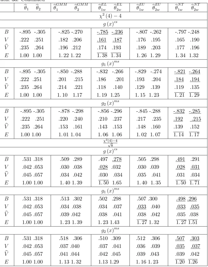
In the simulations we consider median regression estimation of 0 = [1;0:5] in
y=z1 0+" where z1 = [z11; z12] z11=z11+" and z1j (j = 1;2)and " areN(0;1).
The instruments are speci…ed as z2 = [z21; z22] and z2j (j = 1;2) are N(0;1). The
auxiliary information consists of the knowledge of two quantiles for the instrument
z21, that is E[g(x)] = [I(z21 q) p] = 0 with p = [0:1;0:4] . For the correctly
speci…ed case g(x)cs the values of the quantiles are qcs = [ 1:28; 0:25] . For the two moderately misspeci…ed cases g1(x)ms and g2(x)ms we use the same random
seed 123 and specify for n = 50 qms1 = [ 0:70; 0:06] and qms2 = [ 0:55; 0:04]
which yield average p-values (based on 5000 replications) of the EL ratio test for the hypothesis E[g(x)cs] = 0 of 0.200 and 0.114, respectively. For n = 100 we specify
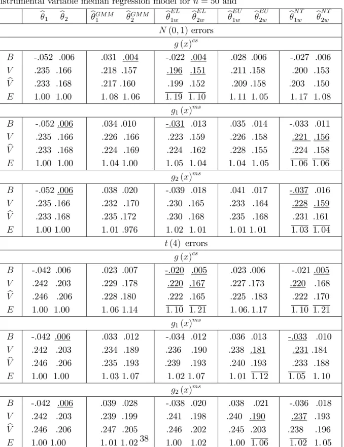
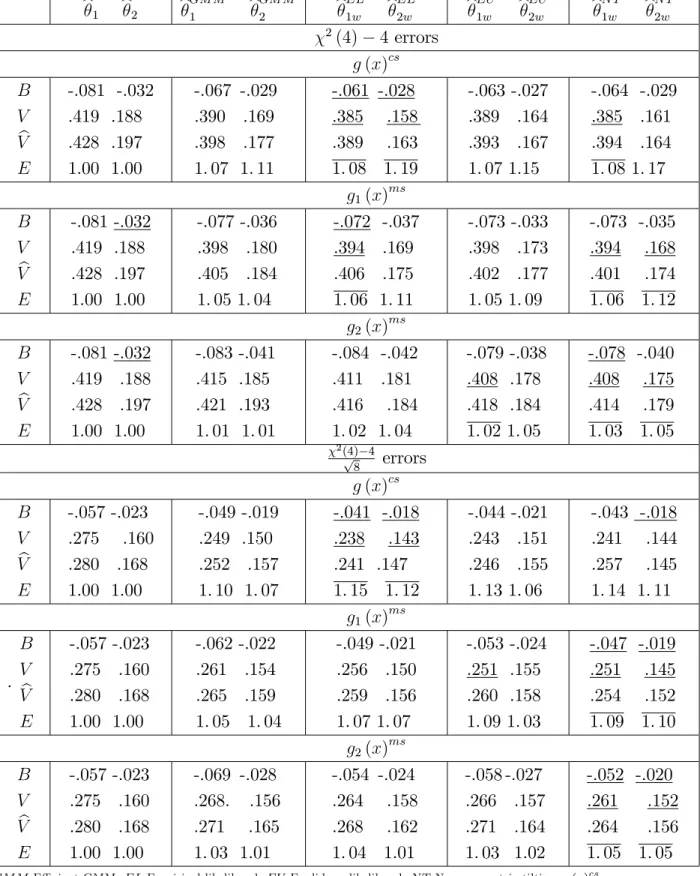
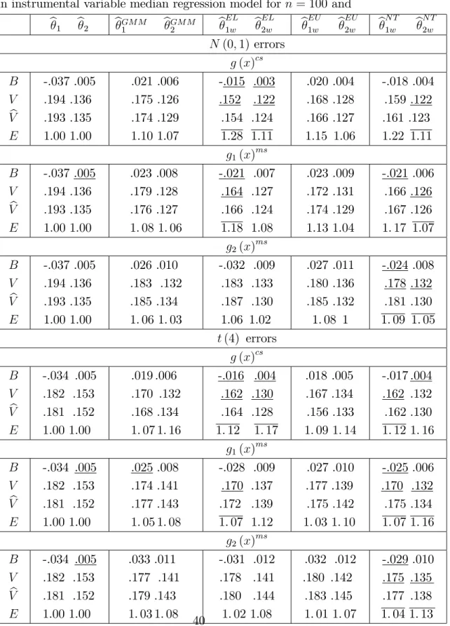
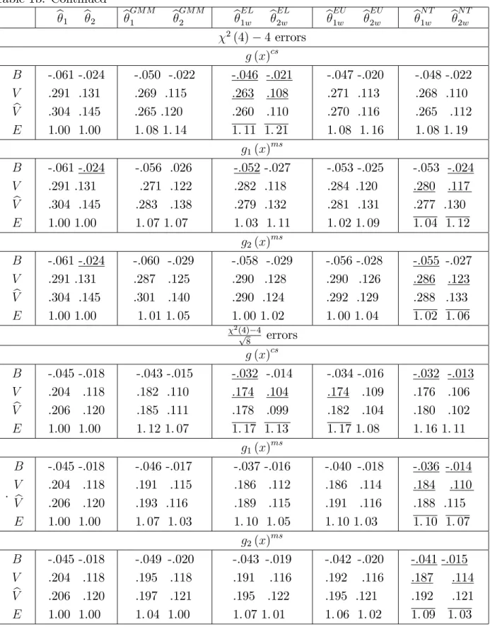
qms1 = [ 0:90; 0:10] and q2ms = [ 0:76; 0:11] which yield average p-values (based on 5000 replications) of the EL ratio test for the hypothesis E[g(x)ms] = 0 of 0.207 and 0.117, respectively. Tables 1a and 1b report also the point estimates of(22) with bandwidth bn chosen by the “Hall-Sheather” rule (Hall and Sheather, 1988).
Tables 1a,b approximately here
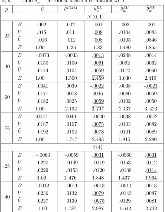
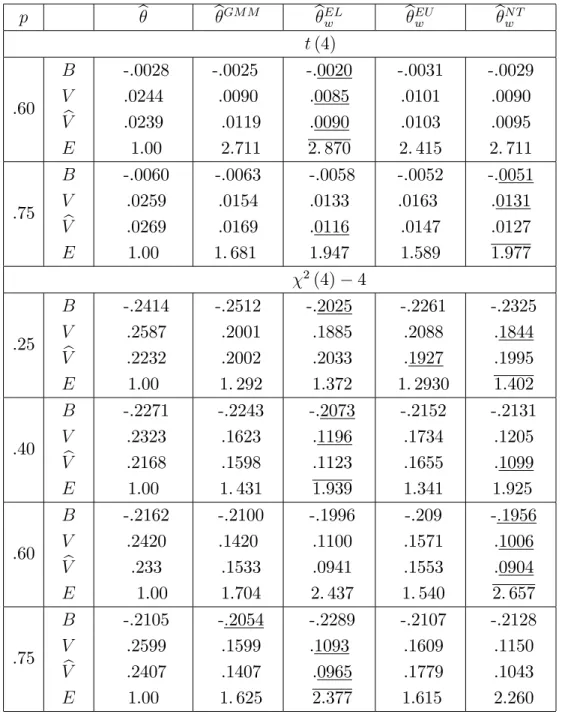
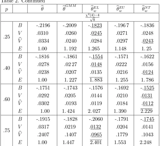
Example 3. Huber’s (1964) location estimatorbfor 0solvesPni=1 xi b =n=
0where ( ) = for j j k and ( ) =ksign( ) for …nitek, or is simply the sample mean for k =1. The following proposition establishes the asymptotic distribution of the weighted location estimatorbw solving Pni=1wbi xi;b = 0:
Proposition 16 Suppose that(1)holds, and (I)xis symmetrically distributed around
0, (II) is an open interval, (III) Ejxj
2 <1, (IV) Ejxj kg(x)k<1. Then n1=2 bw 0 d !N 0; 2g( 0) ; where 2 g( 0) = Z 0+k 0 k x2dF(x) +k2 Z 0 k 1 + Z 1 0+k dF (x) g 1 g = Z 0+k 0 k F(x) 2 ; and g = hR 0+k 0 k x+k R1 0+k R 0 k 1 i g(x)dF (x): Moreover b2g bw a:s ! 2 g( 0) where b2g bw = " n X i=1 b wiI n xi bw k o# 2( n X i=1 b wix2iI n xi bw k o + (23) k2 n X i=1 b wiI n xi bw k o + n X i=1 b wiI n xi bw+k o! b gb 1 b w b g ) ; b g = n X i=1 b wixig(xi)I n xi bw k o +k n X i=1 b wig(xi)I n xi bw+k o k n X i=1 b wig(xi)I n xi bw k o : and bwb is as in (11):
In the simulations we consider estimating the location when thepth population quantile q is known, so that E[g(x)] = E(Ifx qg) p = 0. Table 2 reports the …nite sample properties ofbandbw forp= [0:25;0:40;0:60;0:75] for the casek = 1:5,
including the point estimates Vb of the variance 2g( 0) obtained using (23):
Table 2 approximately here
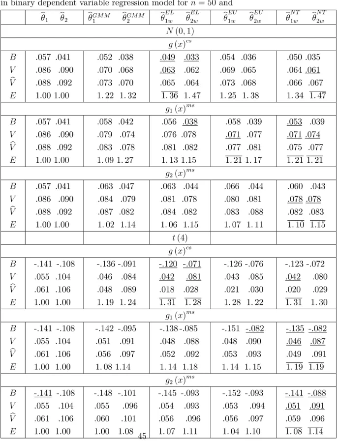
Example 4 Let x = [y; z ] for a binary variable y 2 f0;1g and F ( ) denote the cumulative density function with f( ) and f0( ) to denote its density and …rst
derivative. For example for F( ) = ( ) that is the cumulative distribution of a standard normal we have the standard probit model. An M-estimator (optimally weighted Z estimator) b for 0 solves Pni=1 xi;b =n = 0, where (xi; ) :=
(yi F (zi ))f(zi )zi=F(zi )F ( zi ), where, with a slight abuse of notation,
F ( zi ) = 1 F(zi ) The following proposition establishes the asymptotic dis-tribution of the weighted M-estimatorbw solving Pni=1wbi xi;bw = 0:
Proposition 17 Suppose that(1)holds and (I) compact,Esup 2Fkf(z )=F(z )
F( z )k <1, (II) Ekzk2 < 1, (III) E(zz ) is nonsingular, (IV) there exists a
neighbourhood N0 of 0 such that EsupN0k (x; )g(x)k < 1, (V) p0 2 intf g.
Then n1=2 bw 0 d !N(0; F g( 0)); where F g( 0) = [E( 0(x; 0))] 1 fE( 0(x; 0)) E[(y F (z 0)) (z 0)=F( z 0)zg(x) ] 1E[(y F (z 0)) (z 0)=F ( z 0)zig(x) ] [E( 0(x; 0))] 1 ; E( 0(x; 0)) = E[ (z 0) ( z 0)zz ]and ( ) =f( )=F ( ). MoreoverbF g bw a:s: ! F g( 0), where bF g bw = xb i;bw 1 b w ( b xi;bw b w " n X i=1 b wi yi F zibw zibw =F zibw zig(xi) ]bwb1 " n X i=1 b wi yi F zibw zibw =F zibw zig(xi) # ) b xi;bw 1 b w ; (24) and xb i;bw b w =Pni=1wbi zibw zibw zizi:
In the simulations we consider estimating 0 = [1;0:5] with z = [1; z1] , and z1
is N(0;1). The auxiliary information consists of the knowledge of the conditional mean of y given z 0, that is E[g(x)] = E(yjz 0) +; E(yjz <0) = 0. For the correctly speci…ed case g(x)cs the approximate values of cs
+; cs are
[0:91;0:71] for N(0;1) errors (i.e. standard probit), [0:87;0:70] for t(4) errors,
[0:62;0:49] for centred 2(4) errors, and [0:97;0:68] for standardised 2(4) errors.
For the two moderately misspeci…ed cases g1(x)ms and g2(x) we use use the same
random seed 123 and specify forn = 50 [0:74;0:62] and [0:71;0:59] for the N(0;1)
case, [0:71;0:60] and [0:67;0:57] for the t(4) case, [0:45;0:35] and [0:41;0:33] for the centred 2(4) case, and …nally [80;60] and [77;56] for the standardised 2(4)
case. With these values the average p-values (based on 5000 replications) of the EL ratio test for the hypothesis E[g(x)cs] = 0 are, respectively, 0.195 and 0.111, 0.216 and 0.114, 0.197 and 0.115 and …nally 0.216 and 0.112. For n = 100 we specify
ms
+1; ms1 = [0:78;0:67] and [0:76;0:65] for the N(0;1) case, [0:75;0:64] and
[0:73;0:61] for thet(4)case,[0:50;0:40] and [0:47;0:39] for the centred 2(4) case,
values the average p-values (based on 5000 replications) of the EL ratio test for the hypothesis E[g(x)ms] = 0 are, respectively, 0.211 and 0.119, 0.221 and 0.111, 0.204 and 0.123 and …nally 0.219 and 0.112.
We also consider the bias corrected M and WM estimators, that isn1=2 b
w Biasd bw
where Biasd bw is a consistent estimator (see (18)) of
Biashn1=2 bw 0 i =fE[ (v0) ( v0)zz ]g 1 E (y F (v0))2 (v0) (25) ( v0)zz =F(v0)F ( v0) + (y F (v0))f0(v0)zz =F(v0)F ( v0)] fE[ (v0) ( v0)zz ]g 1[f(v0) (y F (v0))z]=F (v0)F ( v0) =n1=2+ E ( 3 k X j=1 (v0) ( v0)f(v0)f0(v0)zz z(j) ) fE[ (v0) ( v0)zz ]g 1=2n1=2 fE[ (v0) ( v0)zz ]g 1 E (y F (v0))2 (v0) ( v0)zz =F(v0)F ( v0) + (y F(v0))f0(v0)zz =F (v0)F ( v0)]fE[ (v0) ( v0)zz ]g 1 E (y F (z 0)) (z 0)=F( z 0)zg (x) g (x) =n1=2+ fE[ (v0) ( v0)zz ]g 1 E f (v0) (y F (v0))ztr g (x)g (x) E (y F (z 0)) (z 0)=F ( z 0)zg (x) E g (x)tr g (x)g (x) =n1=2;
where v0 =z 0, z(j) is the jth component of z, and
g (x) =h yI(z >0) +0 = +0 1 +0 1=2; yI(z 0) 0 = 0 1 0 1=2i :
The GMM bias corrected estimator isn1=2 b
GM M Biasd bGM M whereBiasd bGM M
is a consistent estimator of Biashn1=2 bGM M 0 i =Biashn1=2 bw 0 i fE[ (v0) ( v0)zz ]g 1 E (y F (v0)) 2 (v0) ( v0)zz =F(v0)F( v0) [E( (v0) ( v0)zz ) (I (v0) ( v0)zz )] 1E[ (v0) ( v0)zz ]g (x) =n1=2 E f(v0) (y F(v0))zg (x) =F (v0)F ( v0) [E( (v0) ( v0)zz ) (I (v0) ( v0)zz )] 1E[ (v0) ( v0)zz ]g (x) =n1=2+fE[ (v0) ( v0)zz ]g 1 fE[ (v0) ( v0)zz ]g 1 [E( (v0) ( v0)zz ) (I (v0) ( v0)zz )] 1 fE[ (v0) ( v0)zz ]g 1 E (y F (v0))2 (v0) ( v0)=zz =F(v0)F ( v0) + (y F(v0))f0(v0)zz =F (v0)F ( v0)] [E( (v0) ( v0)zz ) (I (v0) ( v0)zz )] 1 E( (v0) ( v0)zz )g (x) =n1=2:
Tables 3a,b and 4a,b report, respectively, the …nite sample properties ofb,bw,bGM M
and their bias corrected versionsbc4,bcw,bcGM M as well as the point estimates Vb of
the variance F g( 0) obtained using (24) with correct and moderately misspeci…ed
auxiliary information.
Tables 3 a,b 4 a,b approximately here
We …rst discuss the results of Tables1a- 4b in the case of correctly speci…ed auxil-iary information. First all of the three WM-estimators have …nite sample biases that are smaller than those of the original M and GMM estimators. The bias reduction seems to be a little more substantial in the case of symmetric distributions. Second, as clearly expected from Theorems 4-6, all of the three WM estimators have …nite sample variances that are uniformly smaller than those of usual M-estimators, and are typically smaller than those of GMM estimators. The e¢ ciency gain (i.e. the mag-nitude of the variance reduction) of the proposed estimators depends on the type of estimation considered, on the relevance of the auxiliary information and on the shape of the distribution of the observations. Third the variance estimators (22) (24)
work remarkably well with symmetric distributions and both EL and NT weights. Fourth the bias correction is very e¤ective and removes almost completely the …nite sample bias for symmetric distributions and drastically reduces that for skewed dis-tributions. The variances of the bias corrected estimators are also reduced. Fifth among the three WM estimators considered, those based on EL weights have an edge over those based on NT and EU weights in terms of e¢ ciency. They also seem to have an edge in terms of …nite sample bias. This result is interesting because not only con…rms the small bias property of EL based WM-estimators for the case of smooth estimating equations (see Section 3.3), but also because it suggests that this property seems to be holding also for nonsmooth estimating equations. Finally these results hold for both sample sizes, suggesting that the asymptotic approximations are reliable for relatively small sample sizes. The only di¤erence is that the biases and variances are slightly larger for n= 50.
We now discuss the results of Tables 1a-4b in the case of moderately misspeci…ed auxiliary information. For the g1(x)ms cases, that is for cases where the degree of
misspeci…cation is relatively low, the results are qualitatively very similar to those obtained with correctly speci…ed auxiliary information, and indicate that although 4The bias corrected version bc of the M-estimatorb isbc =b Biasd b where Biasd b is a
the misspeci…cation has some negative …nite sample e¤ects on both GMM and WM estimators, the WM estimators are still clearly superior to both M and GMM estima-tors in terms of …nite sample bias and e¢ ciency. However WM estimaestima-tors based on EL weights seem to be a¤ected by the misspeci…cation comparatively more than those based on either EU or NT. The “sensitivity” to misspeci…cation of EL is con…rmed and emphasised in the second (stronger) case of misspeci…cation (that is forg2(x)
ms
). In this case, as expected from the discussion in Remark 4, all of the WM estimators are characterised by bigger …nite sample biases, but among them those based on NT weights seems to be less sensitive to the increase in the level of misspeci…cation. The robustness of NT is also re‡ected in the variances, which are now typically smaller than those based on EL weights. Finally under misspeci…cation the bias corrections are not as e¤ective as in the case of correctly speci…ed auxiliary information, but they are still useful to reduce the bias of the WM-estimators. As for the case of correctly speci…ed information these results are robust to the sample size; in the case ofn = 50
EL seems to be a little more sensitive to misspeci…cation.
In sum the results of the simulations can be summarised as follows: if the auxiliary information is correctly speci…ed (or the p-vales of a test statistic used to assess its correctness are above 0.20-0.25) WM-estimators (with or without bias correction) based on EL weights are characterised by the best …nite sample performances both in terms of bias and e¢ ciency. On the other hand if there are some doubts about the “correctness”of the auxiliary information (as suggested, for example, by p-values between 0.10-0.25), then WM estimators with NT weights have the best …nite sample performance.
5
Conclusions
In this paper we have introduced a new class of weighted M-estimators where the weights are obtained from GEL estimation of some auxiliary information about the otherwise unknown distribution of the data. These estimators are e¢ cient in the sense of having a smaller variance than that of standard M-estimators, and also in the sense of having the same asymptotic variance as that of e¢ cient GMM estimators with the same auxiliary information. Compared to the latter however, the estimators of this paper are much simpler to compute. Furthermore in the case of smooth estimating equations the proposed estimators are characterised by a small second order bias property compared to e¢ cient GMM estimators.
The …nite sample behaviour of the weighted M-estimators based on the three most used GEL members (empirical likelihood, Euclidean likelihood and nonpara-metric tilting) has been investigated by means of simulations. The results of the latter suggest that when the auxiliary information is correctly speci…ed the proposed estimators are typically less biased and can be notably more precise than those based on standard M and e¢ cient GMM estimation, with those based on empirical like-lihood being the least biased and more precise. On the other hand when there are some doubts about the accuracy of the auxiliary information weighted M-estimators based on nonparametric tilting seem to be preferrable.
References
Andrews, D. (1994), Empirical processes methods in econometrics, in R. Engle and D. Mcfadden, eds, ‘Handbook of Econometrics’, Vol. 4, Amsterdam: North-Holland.
Baggerly, K. A. (1998), ‘Empirical likelihood as a goodness of …t measure’,Biometrika 85, 535–547.
Brown, B. M. and Chen, S. X. (1998), ‘Combined and least squares empirical likeli-hood’, Annals of the Institute of Statistical Mathematics50, 697–714.
Chamberlain, G. (1987), ‘Asymptotic e¢ ciency in estimation with conditional mo-ment restrictions’, Journal of Econometrics 34, 305–334.
Efron, B. (1981), ‘Nonparametric standard errors and con…dence intervals (with dis-cussion)’,Canadian Journal of Statistics, 9, 139–172.
Hall, P. and Sheather, S. (1988), ‘On the distribution of a studentized quantile’,
Journal of the Royal Statistcal Society B50, 381–391.
Handcock, M., Houvilainen, S. and Rendall, M. (2000), ‘Combining registration sys-tem and survey data to estimate birth probabilities’,Demography 37, 187–192. Hellerstein, J. and Imbens, G. (1999), ‘Imposing moment restrictions from auxiliary
data by weighting’, Review of Economics and Statistics 81, 1–14.
Huber, P. (1964), ‘Robust estimation of a location parameter’,Annals of
Huber, P. (1973), ‘Robust regression: Asymptotics, conjectures and Monte Carlo’,
Annals of Statistics 1, 799–821.
Imbens, G. and Lancaster, T. (1994), ‘Combining micro and macro data in micro-econometric models’,Review of Economic Studies 61, 655–680.
Imbens, G. W., Spady, R. H. and Johnson, P. (1998), ‘Information theoretic ap-proaches to inference in moment condition models’, Econometrica 66, 333–357. Koenker, R. and Basset, G. (1978), ‘Regression quantiles’, Econometrica 46, 33–50. McCullagh, P. (1987), Tensor Methods in Statistics, London: Chapman and Hall. Newey, W. K. and Smith, R. J. (2004), ‘Higher order properties of GMM and
gener-alized empirical likelihood estimators’, Econometrica72, 219–256.
Owen, A. (1991), ‘Empirical likelihood for linear models’, Annals of Statistics 19, 1725–1747.
Owen, A. (2001),Empirical Likelihood, Chapman and Hall.
Parente, P. and Smith, R. (2005), ‘GEL methods for non-smooth moment indicators’. Working paper, University of Warwick.
Pfanzagl, J. and Wefelmeier, W. (1978), ‘A third-order optimum property of the maximum likelihood estimator’, Journal of Multivariate Analysis 8, 1–29. Powell, J. (1986), ‘Symmetrically trimmed least squares estimators for Tobit models’,
Econometrica 54, 1435–1460.
Smith, R. J. (1997), ‘Alternative semi-parametric likelihood approaches to generalised method of moments estimation’,Economic Journal 107, 503–519.
Van der Vaart, A. (1998),Asymptotic Statistics, Cambridge University Press.
Zhang, B. (1995), ‘M-estimation and quantile estimation in the presence of auxiliary information’, Journal of Statistical Planning and Inference44, 77–94.
Appendix
We use the following abbreviations and conventions: let g(xi) = gi, Mn= maxikgik,
(xi; ) = i( ),lim = limn!1andPni=1 =
P
; also CLT, CMT, LIL and (U)S(W)LLN stand for central limit theorem, continuous mapping theorem, law of iterated loga-rithm and (uniform) strong (weak) law of large numbers, respectively.
Proof of Theorem 1. By the …rst Borel-Cantelli lemma Mn = oa:s: n1= so
that on n := :k k n , gi = oa:s:(1) and therefore n Vn a:s: Since
Gn( ) is strictly concave on n it follows that there exists (a:s:) a unique e :=
arg max 2 nGn( ). A Taylor expansion about 0 gives
Gn(0) Gn e = X h e gi+ 2( gi)e gigie=2 i =n e kgk s e 2
wherek k e ,g =Pgi=n and s >0 is the smallest eigenvalue of .
Subtract-ing Gn(0) s e
2
; dividing by e and …nally using LIL one gets e kgk =
Oa:s: n 1=2(log logn)1=2 . Since e =oa:s: n , e2 intf ng a:s: hence the …rst
order condition for an interior maximum @Gn e =@ = 0 is satis…ed a:s: Clearly
e 2 Vn so by concavity of Gn( ) and convexity of Vn it follows that Gn e =
sup 2VnGn( ) which implies the existence of a unique b := arg max 2VnGn( ). Next by Taylor expansion 1 b gi = 1 + 2( gi)b gi where k k b . Since
b Mn = oa:s:(1) maxij 2( gi) + 1j =oa:s:(1) uniformly in i so 1 b gi = 1
b gi+oa:s:(1). Similarly
1=X 1 b gi = 1=n 1 +
X
2( gi)gi=n b= 1=n 1 +Oa:s: n 1log logn ;
by LIL and thus
max
i wbi 1=n 1 +b gi =Oa:s: n
1log logn : (26)
By construction Pwbigi = 0 a:s, so by(26) 0 = g+
P
gigib=n+Oa:s:(n 1log logn).
By SLLNPgigi=n a:s
! and hence by CMTn1=2b= 1Pg
i=n1=2+Oa:s: n 1=2log logn .
Applying CLT and CMT to the latter gives (3). Again by(26)
n1=2 Fbw(x) F (x) = n1=2 Fbn(x) F (x) n1=2
X
Ifxi xgb gi=n+
Oa:s: n 3=2log logn =n1=2 Fbn(x) F (x) n1=2E
h
b giIfxi xg
i
from which (4) follows by CLT, and CMT.
Proof of Theorem 2. Note that by(26)
k w( )k k n( )k(1 +oa:s(1))
uniformly in . By this, the de…nition of the estimator and standard arguments
bw bw w bw + w bw
sup
2 k
n( ) ( )k+oa:s(1) n bw +oa:s(1)
oa:s(1) +oa:s(1)k ( 0)k=oa:s(1):
By (II) it then follows that bw 2 k 0k< a:s: and since is arbitrarybw a:s:
! 0:
Proof of Theorem 3. Let w( ") =
P b
wi i( ") for some " > 0:
By (26) and SLLN we have that w( ") a:s:
! ( "). Then monotonicity of
i( ) implies monotonicity of ( ) and since 0 is the unique root of ( 0 "),
( 0 ")<0< ( 0+") for " su¢ ciently small. It then follows that
w( 0 ")<0< w( 0+") a:s:
whence there exists abw such that w bw a:s:
= 0 and bw a:s
! 0by the continuity of
w( ):
Proof of Theorem 4. LetdGbn(x) := dFbn(x) dF (x). Note that w( ) = ( 0) +ok 0k+ n( ) 1 +b gi +oa:s:(1) = Hw( ) +o(k 0k) + Z ( ( ) ( 0))dGbn(x) + b X[ ( ) ( 0)]gi=n+oa:s:(1); where Hw( ) = ( 0) + n( 0) 1 +b gi : Letn1=2 0 =Op(1); then n1=2 w Hw op(1) + (27) sup k 0k n n1=2 Z ( i( ) i( 0))dGbn(x) + n1=2b X i i( 0) gi=n =A1+A2:
By (II) A1 =op(1) while by (III) (a) and the consistency of there exists a n !0
such that supk 0k nk( i( ) i( 0))gik = op(1). Then by (III) (b) and
dom-inated convergence Esupk 0k nk( ( ) ( 0))gik ! 0 so that by triangle and
Markov inequalities X i i( 0) gi=n X sup k 0k n k( i( ) i( 0))gik=n=op(1);
and A2 = Op(1)op(1) = op(1): Thus n1=2 w is asymptotically equivalent to
n1=2H
w . Lete:= arg min kHw( )k and note that
n1=2Hw = n1=2Hw e +op(1);
which implies that n1=2 e
k k n1=2 e = Co
p(1) and hence
n1=2 e = o
p(1). Thus the distribution of is asymptotically equivalent to
that ofe. Sincebw is n1=2-consistent by assumption, the conclusion follows by CLT
and CMT.
Proof of Theorem 5. Assume that ( ) is nonincreasing in , let yn = 0+
y 0g=n1=2where y 2 <, and w(yn) denote the corresponding weighted estimating
equation. Then by (26), (3) and SLLN
w(yn) = X i(yn) 1 +b gi =n+oa:s:(1) = X i(yn) E[ (yn)g ] 1gi =n+oa:s:(1) = X zin=n+oa:s:(1):
As in Huber (1964) it su¢ ces to show thatlim Prf w(yn) 0g= lim PrfPzin=n 0g=
F (y) for every y, where F ( ) is the standard normal distribution. Let Zin :=
(zin Ez1n)= (z1n)where 2(z1n) =V ar(z1n)and note thatlimn1=2E[z1n= (z1n)] =
y(Huber, 1964, p. 78). Thereforelim PrfPzin=n 0g= lim Pr n 1=2PZin y .
Since the Lindeberg condition limRz
n>n1=2"z
2
ndF (z) = 0 holds for
zn := i(yn) +Ej (yn)j kgk 1 kgk ;
it follows by a CLT for triangular arrays thatlim Pr n 1=2PZ
in y =F (y):
Proof of Theorem 6. By(26) and mean value expansion
0 =Xwbi i bw = X i( 0)=n+ X 0 i( ) bw 0 =n+b X i( 0)gi=n+ b X 0
where k 0k bw 0 from which bw 0 =hX 0i( )=n+X 0i( )b gi=n i 1 X i( 0)=n+ X
i( 0)b gi=n+Oa:s: n 1(log logn) :
Since !a:s 0, using (3), USLLN, LIL and CMT one gets
n1=2b X i( 0)gi=n+E[ ( 0)g ] 1g =oa:s(1); b X 0 i( )gi=n b sup 2N0 X 0 i( )gi=n E 0( )g +
b kE 0( )gk=Oa:s: n 1=2(log logn)
1=2
;
X 0
i( )=n E[ 0( 0)] =oa:s(1):
The conclusion follows by CLT and CMT.
Proof of Theorem 7. By consistency ofbw and WLLN bwb p ! , X b wi i bw i bw V sup 2N0 X ( i( ) i( ) =n E[ ( ) ( ) ]) +op(1) so thatVbwb p
!V. Note that by the stochastic equicontinuity (I) and(26)forl= 1; :::; k
b
wi bw+bnel wbi bw bw +bnel bw =op n
1=2b 1
n ;
whereas by the local di¤erentiability (II) and triangle inequality
bw+bnel =bn el bw 0 =bn +op n 1=2bn1 ;
so that again by triangle inequality bwb l
p
! ( )l l = 1; :::; k. Finally by the consis-tency ofbw, ULLN and the triangle inequality
X b wi i bw i( 0) gi + X b wi i( 0)gi E[ i( 0)gi] X i bw (xi; 0) gi =n+op(1) X sup k 0k n k( i( ) i( 0))gik=n+op(1) =op(1)
so that the conclusion follows by CMT.
Proof of Theorem 8. Recall that the one-step weighted M-estimator for 0 is
b1w =bw hX b wi 0i bw i 1X b wi i bw : (29)
By (26) and a mean value expansion it can be shown that (29) can be written as n1=2 b1 w 0 =n1=2A4n1 P3 j=1Ajn, where A1n = X h i( 0) + i( 0)b gi +oa:s:(1) i =n; A2n = X h i bw i( 0) 0i bw 0 i =n; A3n = b X h i bw i( 0) 0i bw 0 i gi=n; A4n = X h 0 i 1 +b gi+oa:s:(1) i =n: LetF g =E[ ( 0) ( 0) ] E[ ( 0)g ] 1E[ ( 0)g ] ; by CLT, CMT and LLN it follows thatn1=2A 1n d !N(0; F g), n1=2A2n =E[ 0( 0)]n1=2 bw 0 +oa:s(1), n1=2A3n b oa:s:(1) +kE[ ( 0)g]k n1=2 bw 0 =
Oa:s: n 1=2(log logn)1 =2
(oa:s:(1) +Op(1)) =op(1);
and kA4n E 0( 0)k=oa:s(1); whence the results follows by CMT.
Proof of Theorem 9. The arguments of the proof of Theorem 1 apply viz. a. viz. to gi := gi =n1=2, so that it is easy to see that 0 = g +
P
gigib=n+
Oa:s: n 1(log logn)1=2 . Thus the …rst conclusion follows by CLT and CMT. As for
the second conclusion note that
n1=2 Fbw(x) F (x) = n1=2 Fbn(x) F (x) n1=2
X
Ifxi xgb gi=n+
Oa:s: n 3=2(log logn)
1=2 =n1=2 Fbn(x) F (x) n1=2E h b giIfxi xg i +oa:s:(1);
and the result follows again by CLT and CMT.
Proof of Theorem 10. Let gi :=gi =n1=2. Note thatmaxi b gi =oa:s:(1)
so that the proofs of Theorem 2 and 3 are still valid, hence the conclusion.
Proof of Theorem 11. Note that
n1=2Hw( ) = n1=2( 0) +n1=2 n( 0) 1 +b gi
so that by CLT and CMT
n1=2 b 0
d
!N 1E[ (x; 0)g(x) ] 1 ; g
where g is as de…ned in Theorem 4. Furthermore similarly to (27)
n1=2b X i i( 0) gi=n n
1=2b X
i i( 0) gi=n
Thus the …rst conclusion follows as in the proof of Theorem 4. The second conclusion follows as in Theorem 5 using
X
zin=n+E[ ( 0)g ] 1 +op(1):
The third and last conclusion follows using an expansion analogous to that in (28), namely 0 =Xwbi i bw = X i( 0)=n+ X 0 i( ) bw 0 =n+b X i( 0)gi=n+ b X 0
i( )gi bw 0 =n+Oa:s: n 1(log logn) =
X i( 0)=n+ X 0 i( ) bw 0 =n+ X gigi=n 1 g X i( 0)gi=n+ b X 0
i( )gi bw 0 =n+Oa:s: n 1(log logn)
1=2
;
and the rest of the proof is identical to that of Theorem 6.
Proof of Theorem 12. We use tensor notation and indicate arrays by their elements as for example in McCullagh (1987). Thus, for any index sayj,ajis a vector,
ajk is a matrix, etc. We also follow the summation convention, that is for any two
repeated indices, their sum is understood. For 1 a; b; c; ::: q and 1 ; ; ::: k
let
Aabc::: = X gaigibgci::: abc::: =n; abc::: =E giagbigci: ; B 1::: k = X @k i ( 0)=@ 1:::@ k 1:::: k =n; 1:::: k = E @k i ( 0)=@ 1:::@ k ; C 1::: kabc::: = X @k i ( 0)=@ 1:::@ k giag b i::: 1 :::: kabc::: =n; 1:::: kabc::: = E @k i ( 0)=@ 1:::@ k giag b i::: ;
that is Aabc:::, B 1::: k and C 1::: kabc::: represent O
p n 1=2 random arrays of,
re-spectively. higher order moments of the standardised auxiliary information, higher order derivatives of the estimating functions, and of covariances between higher order derivatives of the estimating functions and the higher order arrays of moments of the standardised auxiliary information.
First we obtain a third-order stochastic expansion for ba that solves 0 =Pwb igia.
Recall that wbi = 1 bagia =
P
1 bagia thus using a third order Taylor expansion
of the numerator and of the denominator and some algebra we obtain
0 = X 1 +bbgib 3 bbgbi
2
=2 3 bbgib
3
which can then be inverted to give
ba = Aa+AabAb+
3 abcAbAc=2 AabAbcAc 3AabcAbAc=2 + 3 abcAbAcdAd 4
abcdAbAcAd=3! 2 3
abc cefAbAeAf=2 +O
p n 2 : (30)
Next using (30) we obtain thatwbi has the following stochastic expansion
b wi = 1 gaiA a+ga iA abAb+ 3g a i abcAbAc=2 ga iA abAbcAc 3g a iA abcAbAc=2 + 3g a i abc
AbAcdAd 4 abcdgiaAbAcAd=3! 23gia abc cefAbAeAf=2
3g a ig b iA aAb=2 + 3g a ig b iA a AbcAc + 3 bcdAcAd=2 3g a ig b iA acAbdAcAd=2 2 3g a ig b iA ac bde AcAdAe=2 33giagbi acd befAcAdAeAf=8 + 4giag b ig c iA aAbAc=3! +O p n 2 : (31)
Finally we obtain a third order stochastic expansion forbthat solves0 = Pwbi i b .
By a third order Taylor expansion about 0
0 =Xwbi i +@ i ( 0)=@ b 0 +@2 i ( 0)=@ @ b 0 b 0 =2+
where for notational simplicity i ( 0) = i. By (30) and (31) we get 0 = +X igib Ab+AbcAc+ 3 bcdAcAd=2 AbcAcdAd 3AbcdAcAd=2+ 3A bcdAcAd=2 + 3 bcdAcAdeAe 4 bcdeAcAdAe=3! 2 3 bcd defAcAeAf=2 =n 3 X igibgic Ab+ AbdAd+ 3 bdeAdAe=2 Ac+ AceAe+ 3 cefAeAf=2 =n+ 4 X igibgicAbAcAd=(3!n) +B b 0 + X Bi b 0 gia Aa+AabAb+ 3 abcAbAc=2 AabAbcAc 3A ab bcdAcAd=2 + 3 abcAbAcdAd 2
3 abc cdeAbAdAe=2 4 abcdAbAcAd=3! =n+ 3
X Bi b 0 giagibAaAb=(2n) + b 0 + X b 0 gia A a +AabAb+ 3 abcAbAc=2
AabAbcAc 3Aab bcdAcAd=2 + 3 abcAbAcdAd 23 abc cdeAbAdAe=2
4 abcd AbAcAd=3! =n 3X b 0 giag b i A a +AacAc + 3 acdAcAd=2 Ab+AbdAd+ 3 bdeAdAe=2 =(2n) + 4X b 0 giag b ig c iA aAbAc=(3!n) + B b 0 b 0 =2 + b 0 b 0 =2 X b 0 b 0 giaAa=(2n) + b 0 b 0 b 0 =3! +Op n 2 ;
where =Pi i=n and similarly for B :::. Inverting this expansion we get
b 0 = + aAa+Q2+Q3+Op n 2 ;
where is the matrix inverse of ,
Q2 = C aAa aAabAb 3 a abcAbAc=2 + 3 abAaAb=2+ (32) B B aAa a Aa+ a bAaAb " " 2 " " aAa+ " "a bAaAb =2 ;
and Q3 = B C aAa+ aAabAb+ 3 a abcAbAc=2 3 abAaAb=2 +(33) B B " " +B " " aAa+ "a " Aa "a " bAaAb + B " " # =2 + " a bAaAb=2 " # aAa + C a AabAb 3 abcAbAc=2 + aAab AbcAc+ 3 bcdAcAd=2 3 a
AabcAbAc=2 + abcAbAcdAd 3 abc cdeAcAdAe=2
4 a abcdAbAcAd=3! +C a Aa+ bAaAb a AabAb+ bAacAbAc 3 a abc AbAc+ dAbAcAd =2 B " "+ " "aAa + A =2 " + aAa + bAb " + " cAc =3! :
Proof of Corollary 13. The result follows by direct calculations in (32) using using
E Aab:::Aa1b1::: = ab:::a1b1:::=n; E Aab:::Aa1b1:::Aa2b2::: = ab:::a1b1:::a2b2:::=n2;
E Aab:::Aa1b1:::Aa2b2:::Aa3b3::: = ab:::a1b1:::a2b2:::a3b3:::=n3+ [3] (n 1) ab:::a1b1::: a2b2:::a3b3:::=n2
where [3] = ab:::a1b1::: a2b2:::a3b3:::+ ab:::a2b2::: a1b1:::a3b3:::+ ab:::a3b3::: a1b1:::a2b2:::, and
simple algebra:
Proof of Corollary 14. The result follows by ULLN and CMT as in the proof of Theorem 7.
Proof of Proposition 15. We verify the conditions of Theorems 2 and 4. Note that (I)-(III) andEsup p2 kz2isignpf"igk (1 +p)Ekz2k<1imply by Theorem
2 thatbpw a:s:
! p0. Note also that by the results of Andrews (1994)
X
z2isignpf"i z1i( p p0)=n E[p F"(z1i( p p0)jz)]g
is stochastically equicontinuous; furthermore by CLT
X
z2isignpf"ig=n1=2 d
!N(0; p(1 p)E(z2z02))
so that by the di¤erentiability condition (IV) it can be shown thatn1=2 bpw p0 =