Wall-Resolved Large-Eddy Simulation of Flow Separation Over
NASA Wall-Mounted Hump
Ali Uzun
∗National Institute of Aerospace, Hampton, VA 23666
Mujeeb R. Malik
†NASA Langley Research Center, Hampton, VA 23681
This paper reports the findings from a study that applies wall-resolved large-eddy simulation to investigate flow separation over the NASA wall-mounted hump geometry. Despite its conceptually simple flow configu-ration, this benchmark problem has proven to be a challenging test case for various turbulence simulation methods that have attempted to predict flow separation arising from the adverse pressure gradient on the aft region of the hump. The momentum-thickness Reynolds number of the incoming boundary layer has a value that is near the upper limit achieved by recent direct numerical simulation and large-eddy simulation of in-compressible turbulent boundary layers. The high Reynolds number of the problem necessitates a significant number of grid points for wall-resolved calculations. The present simulations show a significant improve-ment in the separation-bubble length prediction compared to Reynolds-Averaged Navier-Stokes calculations. The current simulations also provide good overall prediction of the skin-friction distribution, including the relaminarization observed over the front portion of the hump due to the strong favorable pressure gradient. We discuss a number of problems that were encountered during the course of this work and present possible solutions. A systematic study regarding the effect of domain span, subgrid-scale model, tunnel back pres-sure, upstream boundary layer conditions and grid refinement is performed. The predicted separation-bubble length is found to be sensitive to the span of the domain. Despite the large number of grid points used in the simulations, some differences between the predictions and experimental observations still exist (particularly for Reynolds stresses) in the case of the wide-span simulation, suggesting that additional grid resolution may be required.
I.
Introduction
Smooth-body flow separation is an important problem of practical interest, due to its appearance in many tech-nological applications. The problem involves a boundary layer attached to a solid surface, which becomes detached from the surface after interaction with an adverse pressure gradient generated by a change in body contour or the pres-ence of a shock. This phenomenon commonly occurs in flows over aircraft wings, helicopter rotors, turbomachinery blades and high-lift configurations, to name a few. Separation often leads to increased aerodynamic drag, stall and re-duced system performance. Such separated flows are generally difficult to predict because they involve high Reynolds number turbulence. These high Reynolds number flows have been traditionally studied using techniques such as Reynolds-Averaged Navier-Stokes (RANS) calculations, wall-modeled large-eddy simulations (WMLES) or hybrid RANS-LES type approaches. In the case of RANS, available turbulence models commonly fail to properly account for non-equilibrium effects in separated flows, and therefore leave room for improvement. An example demonstrating the failure of RANS in a low-speed flow separation problem can be found in the paper by Rumsey et al.1The problem
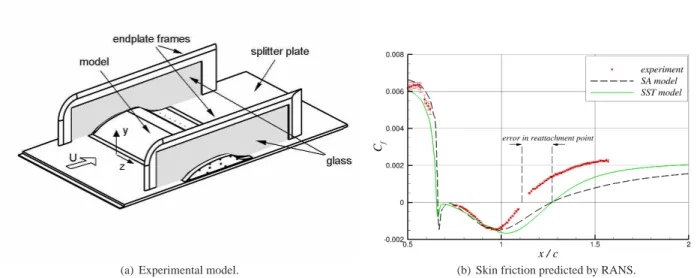
involves a wall-mounted hump geometry, also known as the NASA hump, representative of the upper surface of an airfoil, as depicted in Figure1(a). The aft portion of the hump generates an adverse pressure gradient, which causes boundary layer separation atx/c ≈ 0.665and flow reattachment further downstream, atx/c ≈ 1.11. Figure1(b) depicts the failure of RANS in the prediction of separation-bubble length, which is overestimated by about35%.
The same benchmark problem has also been studied using WMLES (e.g., see the studies of Avdis et al.,3Shur et al.,4 Park,5 Duda and Fares,6 Iyer and Malik7). In WMLES, the critical near-wall region of the turbulent boundary
∗Senior Research Scientist, Senior Member AIAA.
†Senior Aerodynamicist, Computational AeroSciences Branch, MS 128, Fellow AIAA.
(a) Experimental model. (b) Skin friction predicted by RANS.
Figure 1. NASA wall-mounted hump experiment2.
layer is modeled, rather than resolved, to avoid stringent grid resolution requirements. Despite generally promising results from these studies, the overall success of WMLES at present can be characterized as mixed at best. The success or failure of WMLES in separated flows strongly depends on the accuracy of the wall model employed in the near-wall region. While wall models have been proposed for both equilibrium and non-equilibrium conditions, the true performance of some wall models is hard to assess since certain critical information, such as surface skin-friction distribution, is not always provided or grid convergence of the solution is not clearly demonstrated. From aerodynamic considerations, the skin-friction distribution is one of the most important quantities and WMLES usually does not yield satisfactory results for this quantity. The recent study by Iyer and Malik7showed in particular that for the NASA wall-hump problem, the skin friction predicted by a WMLES based on an equilibrium wall model needed improvement. For the current configuration, there is also a region of strong favorable pressure gradient over the front part of the hump, where RANS and WMLES both tend to yield inaccurate skin-friction distributions.
There have also been studies of the wall-mounted hump problem in which traditional LES was applied without any wall models (e.g., see the studies by You et al.8 and Franck and Colonius9). However, careful examination of
these studies reveals that the near-wall grid resolutions are not sufficient. In particular, the boundary layer resolution in wall units reported by You et al.8 cannot be attained with the number of grid points used (about7.5million points
total) and therefore, is in error. As will be discussed, a lot more grid points are needed for a wall-resolved simulation at high Reynolds number. Even though these prior studies have reported some encouraging results, we believe that the practice of performing an LES using an under-resolved grid without wall modeling is ill-founded because the near-wall region of the boundary layer has to be modeled if the grid resolution is not sufficient to properly resolve that region.
A survey of the current literature confirms the lack of well-resolved turbulence simulations for complex separated flows at high Reynolds number. To our knowledge, for the NASA hump problem, the best-resolved simulation prior to the current work is the coarse-grid “DNS” performed by Postl and Fasel.10 This DNS is labeled “coarse-grid” because the resolution in wall units is more in line with a wall-resolved LES (WRLES) rather than DNS. A total of 210million points were used in their DNS with a relatively small spanwise domain of0.142c, wherecis the hump chord length. Despite reasonable overall agreement, the predicted separation-bubble length was found to be larger than that in the experiment. A more recent WRLES was conducted for the same problem by Yeh et al.11This WRLES was performed at half the experimental Reynolds number and for a spanwise domain of0.2c, using93million grid points. The predicted separation-bubble length was larger than the experimental measurement by about20%.
Well-resolved simulations of complex separated flows are very rare in the literature mainly because of the ex-tensive computational resources required. To address this deficiency and generate detailed data needed for a better understanding of the problem at hand, WRLES of the NASA hump benchmark test case is performed using up to850 million grid points in the present work. A systematic study regarding the effect of domain span, subgrid-scale (SGS) model, tunnel back pressure, upstream boundary layer conditions and grid refinement on the results is performed. As will be seen, the separation-bubble length is found to be sensitive to the span of the computational domain. This paper
will discuss the main problems that were encountered during the course of this work and present viable solutions.
II.
Computational Methodology
The code used in the present study solves the unsteady fully three-dimensional compressible Navier-Stokes equa-tions discretized on multi-block structured and overset grids. A turbulence simulation can be run in the form of direct numerical simulation (DNS), large-eddy simulation (LES), delayed detached eddy simulation (DDES) or unsteady Reynolds-Averaged Navier-Stokes (URANS) calculation.
The code employs an optimized prefactored fourth-order compact finite-difference scheme12 to compute all
spa-tial derivatives. This optimized scheme offers improved dispersion characteristics compared to standard sixth- and eighth-order compact schemes.13 To eliminate spurious high-frequency numerical oscillations that may arise from
several sources (such as grid stretching, unresolved fluctuations and approximation of physical boundary conditions) and ensure numerical stability during the simulation, we also employ a sixth-order compact filtering scheme.14, 15
The overset-grid capability is useful in meshing complex geometries and avoiding grid-point singularities. To main-tain high-order accuracy throughout the entire computational domain, we perform a sixth-order accurate explicit La-grangian interpolation16 whenever overset grids are used. A Beam-Warming type approximately factorized implicit scheme is used for the time advancement.17 More details of the simulation methodology are given in related publica-tions.18–21 Successful applications of the methodology to some wall-bounded flow problems can be found in papers by Uzun and coworkers.18, 22, 23
III.
Test Case: Flow Separation Over NASA Wall-Mounted Hump
The test case studied in this paper involves low-speed flow separation over a wall-mounted hump geometry, also known as the NASA hump, representative of the upper surface of an airfoil, as depicted in Figure1(a). In the follow-ing sub-sections, we provide a description of the experimental setup and computational modelfollow-ing, discuss the main problems encountered and examine the simulation results.
A. Experimental Setup and Computational Modeling
An experimental investigation of the NASA wall-mounted hump, depicted in Figure1a, was conducted by Greenblatt et al.2 The reference length scale is taken as the hump chord length,c = 420mm. The Reynolds number based on
freestream velocity and chord length has a value ofRec ≈936,000. As will be discussed, there is some uncertainty regarding the momentum-thickness Reynolds number of the incoming boundary layer, Reθ, measured about two chord lengths upstream of the hump. The experimental study originally reported a value ofReθ= 7200. Our estimate for this parameter isReθ ≈ 6454, as discussed in sectionIII.B.1. Regardless of the exact value, suchReθ values are relatively high from a computational point of view, as the highestReθ achieved by DNS24 and WRLES25 for incompressible turbulent boundary layers at the time of this writing is6500and8300, respectively. Because of the highReθ, a significant number of grid points is needed for the wall-resolved calculations in the present study.
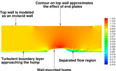
The freestream Mach number upstream of the hump is0.1. The experimental setup includes end plates attached to the model as depicted in Figure 1a. Modeling of these end plates in a wall-resolved simulation would prove computationally very expensive. The simulations therefore use a periodic spanwise domain. The simulations consider two spans of0.2cand0.4c. The distance between the end plates in the experiment is1.4c. The flow blockage effect caused by the end plates in the experiment causes additional flow acceleration over the hump. A specially contoured top wall that mimics this effect is therefore used here. Figure2 depicts the main features of the problem under investigation and also shows the specially contoured top wall. More details can be found on the NASA Turbulence Modeling Resource website at: http://turbmodels.larc.nasa.gov/nasahump val.htmla. The experimental chord-based
Reynolds number is matched exactly in all simulations. As will be discussed, the experimental Mach number is also matched exactly in the narrow-span case, but is increased to0.2for the wide-span case to speed up the calculations since the computational cost increases with decreasing Mach number for our compressible flow solver. Further details of the simulations are provided in sectionIII.C.
Figure 2. Main features of the NASA hump problem depicted in terms of instantaneous normalized streamwise velocity contours. (Only part of the full streamwise extent of the computational domain is shown.)
B. Problems Encountered
Before examining the computational results, we discuss a number of important problems that were encountered during the course of this work and present possible solutions.
1. Experimental Incoming Boundary Layer Details
The first problem is concerned with the details of the incoming boundary layer measured atx/c = −2.14 in the experiment, wherexdenotes the streamwise distance measured from the hump leading edge (located atx/c = 0). Although the experimental study2 originally reported a momentum-thickness Reynolds number ofRe
θ = 7200at
that location, the momentum-thickness integral of the mean velocity profile obtained from a RANS calculation (that matches the experimental mean velocity profile26) provides a lower value ofRe
θ ≈6454. The comparison between this RANS mean velocity profile and the experimental measurement is shown in Figure3. Moreover, the experimental skin-friction measurement27taken atx/c=−2.14provides a normalized friction velocity value ofu
τ/u∞≈0.0378.
The corresponding Reynolds number based on the experimental boundary layer thickness and friction velocity is
Reτ ≈2225. For a canonical flat-plate turbulent boundary layer, this friction velocity corresponds toReθ ≈5000. Flat-plate turbulent boundary layer data available from DNS24 and WRLES25 were examined to determine theReθ corresponding to the reported skin-friction velocity. Figure4shows the flat-plate turbulent boundary layer profiles from these DNS and LES for5000≤Reθ≤7000in the form of mean streamwise velocity and streamwise turbulence intensity, and the comparison with the experimental measurement. We see that none of the computational profiles are an exact match to the experimental profile. These findings suggest that the boundary layer upstream of the hump in the experiment (atx/c=−2.14) is perhaps not precisely a flat-plate turbulent boundary layer.
Given this uncertainty in upstream boundary layer conditions, we considered two options for the simulations. The first option is to match the reported upstream skin friction in the experiment and hence setReθ = 5000for the incoming boundary layer upstream of the hump. A turbulent inflow generation technique that generates a canonical flat-plate turbulent boundary layer atReθ = 5000can be employed for this purpose. The second option is to take the mean velocity profile available from RANS and add the turbulent fluctuations to this mean profile using an inflow generation technique. We use only the first option for the narrow-span calculation but explore both options for the wide-span case. For the turbulent inflow generation, a specific version of the rescaling-recycling technique, discussed in Uzun and Hussaini,28is used. This inflow generation method is additionally augmented with several modifications proposed by Morgan et al.29 to eliminate possible energetic low frequencies that may be artificially introduced by the turbulent inflow generation technique. The distance between the inlet and recycle stations is15times the incoming boundary layer thickness. This distance is in the typically recommended range.
y / c 0 0.02 0.04 0.06 0.08 0.1 0.12 0.14 0.16 0 0.2 0.4 0.6 0.8 1
wall hump experiment inflow RANS
U / Uref
Figure 3. Comparison between RANS-predicted mean streamwise velocity profile and experimental measurement atx/c=−2.14.
2. Grid Size for WRLES
The second problem is concerned with maintaining a reasonable grid resolution while keeping the total number of grid points at a manageable level for the available computational resources. A proper WRLES requires a significant grid resolution in the near-wall region of the turbulent boundary layer. This is because energy-containing small eddies in the near-wall region need to be resolved and are not accounted for accurately by the SGS modeling. Our preliminary tests on a canonical flat-plate turbulent boundary layer show that the present methodology requires a streamwise resolution of∆x+
≈25, a spanwise resolution of∆z+
≈12.5, and a wall-normal resolution of∆y+
≈1on the wall, where the superscript+indicates wall units, in order to predict the wall skin friction accurately. This resolution approaches the typical values used in DNS of turbulent boundary layers.24 As will be seen, these values predict the skin friction
reasonably well (within a few percent) in the attached-flow region prior to separation.
y+ 10-1 100 101 102 103 104 0 5 10 15 20 25
30 wall hump experiment inflow
flat plate DNS, Re = 5000 flat plate DNS, Re = 6500 flat plate LES, Re = 7000
U+
(a) Mean streamwise velocity profiles in wall units.
y+ 10-1 100 101 102 103 104 0 0.5 1 1.5 2 2.5 3
wall hump experiment inflow flat plate DNS, Re = 5000 flat plate DNS, Re = 6500 flat plate LES, Re = 7000
u+rms
(b) Streamwise turbulence intensity profiles in wall units.
Figure 4. Comparison of experimental inflow measurements with flat-plate turbulent boundary layer data from DNS24and LES25. Maintaining this grid resolution all the way to the edge of the turbulent boundary layer in the present problem be-comes prohibitively expensive because of computational resource limitations. A reasonable compromise is to maintain the fine grid spacings only in the near-wall region, say up to abouty+
≈200, and then coarsen both the streamwise and spanwise resolution by a factor of two in the outer region away from the wall. This is the strategy adopted here. In the near-wall region, the turbulent boundary layer approaching the hump is resolved using∆x+
≈25,∆z+
∆y+
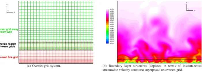
≈0.8on the wall. Similar resolution is maintained for the boundary layer over the hump. The flow solver has overset-grid capability, and the inner and outer region grids communicate by means of sixth-order accurate overset-grid interpolation. Figure5shows a cross-section of the two-level overset-grid system at a streamwise location upstream of the hump and the instantaneous boundary layer structures superposed on the overset-grid. The small structures near the wall are resolved by the near-wall fine grid while the coarser outer grid seems appropriate for the larger struc-tures away from the wall. A similar overset-grid strategy was successfully tested in the study of Tollmien-Schlichting instability waves developing in a subsonic laminar boundary layer. Comparison with the solution of the parabolized stability equations showed that the overset-grid technique did not introduce an error in the computation of instability waves.
(a) Overset-grid system. (b) Boundary layer structures (depicted in terms of instantaneous streamwise velocity contours) superposed on overset-grid.
Figure 5. Two-level overset-grid system atx/c=−2. For better clarity, the vertical scale in the left and right figures is not the same.
3. Acoustic Resonance and Its Effect on Turbulent Inflow Generation
The third problem is concerned with the turbulent inflow generation in the region upstream of the hump. In our initial simulations, we attempted to employ a rescaling-recycling technique28 to generate a turbulent incoming boundary
layer at about two chord lengths upstream of the hump. However, this strategy did not work as expected in this region because it did not produce a boundary layer with properties similar to those of a canonical flat-plate turbulent boundary layer. Upon further investigation, an acoustic resonance phenomenon was determined to be responsible for this issue. We found that the acoustic disturbances generated by the flow going over the hump get trapped inside the closed tunnel and excite an acoustic resonance, eventually giving rise to trapped waves in front of the hump, as depicted in Figure6(a). These trapped acoustic waves continuously propagate up and down in front of the hump, precisely in the region where information is rescaled and recycled for the turbulent inflow generation. Upon impingement onto the lower wall, they instantaneously create local adverse or favorable pressure gradients, thus violating the zero pressure gradient assumption on which the inflow generation technique is based. Wind-tunnel acoustic resonance is a phenomenon that is known to occur in physical experiments and has previously motivated Ikeda et al.30 to perform a computational investigation of the wind-tunnel acoustic resonance induced by the flow over a 2-D airfoil.
We considered two possible solutions to this problem. The first option is to perform an auxiliary simulation for a turbulent boundary layer developing on a flat plate and use the unsteady information at a given streamwise station (where the local momentum-thickness of the boundary layer may correspond to a value such asReθ = 5000) from this calculation as the inflow conditions for the hump simulation. This option was in fact employed in the narrow-span simulation. However, this strategy further increases the computational cost and complexity as it requires two simulations to be carried out simultaneously. A second and computationally cheaper option is to suppress the acoustic resonance by adding a damping term to the right-hand side of the governing equations. The damping term is only active in the vicinity of the top tunnel wall and has the form ofσ(q−q), whereσis a function of the vertical distance
and controls the strength of the damping term.σis zero in the region where the damping term is inactive. The damping term forces the numerical solution,q, in the chosen region toward a reference state, such as a running time-average of
the local flow,q. The region in which the damping term is applied is sufficiently away from the turbulence-containing
region, hence the turbulent fluctuations in the attached and separated regions are not affected by this term. Figure 6(b) shows a schematic of this approach and demonstrates that the damping term is indeed effective in suppressing the acoustic resonance. With the troublesome trapped acoustic waves out of the picture, the inflow generation technique
can work successfully in the region upstream of the hump and there is no need for an auxiliary simulation. This approach is used in the wide-span calculations.
(a) Waves trapped upstream of hump. (b) Suppression of acoustic resonance.
Figure 6. Acoustic resonance giving rise to trapped waves and its suppression by use of a special damping term.
C. Simulation Details
The experimental chord-based Reynolds number (i.e.,Rec = 936,000) is matched exactly in all simulations. The simulations consider two spans of0.2cand0.4c. The experimental Mach number of0.1is also matched in the narrow-span calculation, but is increased to0.2for the wide-span calculations to reduce the computational time. The time step of all simulations is2.5×10−4
c/aref, wherearefis the reference speed of sound. The reference freestream conditions are taken atx/c=−2.14. With this time step, the maximum CFL number is about17. Three subiterations per time step are applied for the fully implicit time advancement scheme. Our experience shows that the maximum CFL number in the simulation should be kept below a maximum of approximately25to ensure sufficient temporal accuracy from the second-order implicit time advancement scheme. This was determined by examining the skin-friction predictions in a canonical flat-plate turbulent boundary layer obtained with different CFL numbers.
A schematic of the computational domain is shown in Figure2. This figure depicts part of the full streamwise extent of the domain. To reiterate, the hump leading edge is located atx/c= 0, while the inlet boundary of the hump domain is atx/c =−2.14. The physical region of interest in the hump domain extends up tox/c = 1.6. A sponge zone is placed downstream of the physical region of interest. The outflow boundary of the computational domain is placed at the end of the sponge zone and is located atx/c = 4. The back pressure on the outflow boundary is set slightly below the upstream pressure (see sectionIII.D.2). The top wall of the computational domain is treated as an inviscid wall while viscous adiabatic boundary conditions are imposed on the lower wall. Characteristic boundary conditions are applied at the outflow boundary. The inflow boundary is based on characteristic relaxation boundary conditions31 that inject turbulent fluctuations (generated by the inflow generation technique) in the boundary layer while allowing upstream-traveling waves to exit the domain. The turbulent boundary layer approaching the hump is resolved using90to100points in the wall-normal direction. Flow acceleration over the hump causes a significant thinning of the boundary layer. The thinnest part of the boundary layer over the hump is resolved using a minimum of about30points in the wall-normal direction.
1. Narrow-Span Calculation
As mentioned earlier, the narrow-span calculation involves an auxiliary simulation that computes the turbulent bound-ary layer developing over a flat plate and a main simulation for the flow over the hump. An instantaneous plane extracted from the flat-plate domain atReθ = 5000is injected as the inflow conditions on the upstream boundary of the hump domain. The flow solver runs on the two domains simultaneously and generates the inflow conditions for the hump domain on the fly. The flat-plate domain contains about90million points while the wall hump domain contains about210million points. The two-level overset-grid strategy is used for both domains. The static Vreman SGS model32is employed with a fixed model coefficient of0.025. Statistical results are averaged over about10chord
flow times, where one chord flow time unit (i.e.,c/Uref) is defined as the time it takes for the reference freestream velocity,Uref, to travel one chord length.
2. Wide-Span Calculations
The wide-span grid is obtained by doubling the spanwise extent of the narrow-span grid while keeping the same resolution as for the narrow-span grid. In the wide-span calculations, the tunnel acoustic resonance is suppressed by the use of a damping term in the vicinity of the top wall and the turbulent inflow generation is done upstream of the hump within the main simulation. The number of points in the wide-span grid is about420million. Because of the increased grid size, the Mach number is increased from0.1 to0.2 to speed up the calculation and help reduce the computational cost. The time step is kept the same as that in the narrow-span case (2.5×10⁻⁴c/aref). Doubling the
Mach number from0.1to0.2means that the flow in the wide-span case convects twice as fast. The inflow and outflow boundary locations are the same as those in the narrow-span case. A number of calculations are performed for the wide-span case. These calculations reveal the effect of SGS model, tunnel back pressure, upstream boundary layer
Reθand grid refinement on the numerical predictions. Statistical results are typically averaged over about30c/Uref.
D. Results
We now examine the simulation results and make comparisons with the experimental measurements.
1. Narrow-Span Calculation
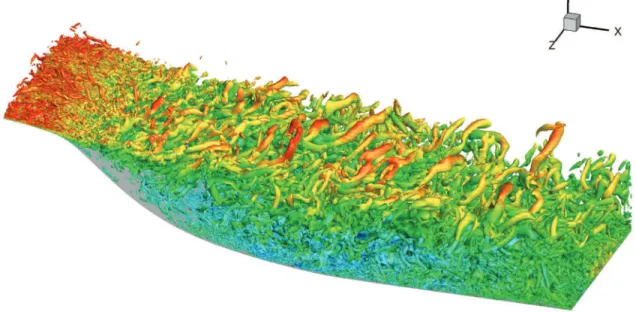
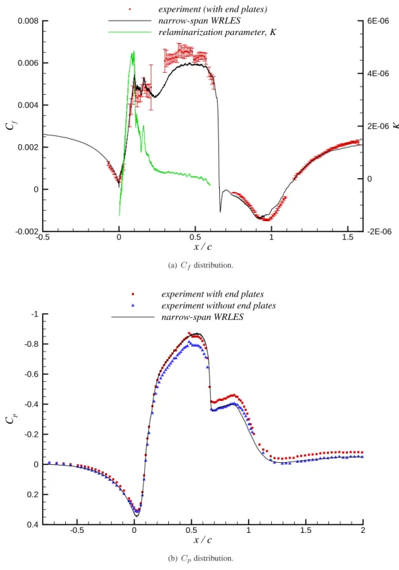
The results from the narrow-span WRLES are analyzed first. Figure7depicts the complex nature of the separated flow in the aft portion of the wall-mounted hump. The initially thin separated free shear layer quickly gives rise to the formation of large-scale structures, which in turn govern the dynamics of the shear layer growth and dictate the reattachment location of the separated flow. Figure8 shows the skin-friction and pressure coefficients and the comparison with the experimental measurement. The skin-friction and pressure coefficients are defined as
Cf = τwall 1 2ρrefU 2 ref and Cp= p−pref 1 2ρrefU 2 ref (1)
where τwall is the viscous wall shear stress, ρandp, respectively, are the density and pressure, and the subscript ref denotes the reference freestream conditions atx/c = −2.14. The WRLES results are based on the mean flow obtained by averaging the unsteady flow in time and along the span. The skin-friction comparison figure includes the error bars for the experimental data. The overallCf distribution and the separation-bubble length are predicted by the simulation reasonably well. The separation and reattachment locations in the simulation are determined by the streamwise locations at whichCf becomes zero. The predicted separation and reattachment locations based on this criterion are fairly close to the experimentally observed values. The separation location is atx/c≈0.665in the experiment and atx/c ≈0.659in the simulation, while the reattachment is atx/c ≈1.11in the experiment and at
x/c= 1.095in the simulation. The underprediction ofCf in the peak region prior to flow separation is primarily an SGS model effect, as will be demonstrated in the wide-span calculations.
Of particular note is the plateau in the measured skin friction at 0.1 < x/c < 0.2, which is predicted well by the present simulation. This plateau is presumably caused by a tendency toward relaminarization due to the strong favorable pressure gradient in this region. Figure8a includes the relaminarization parameter,K, and shows that this parameter reaches its peak just before the plateau inCf. The original definition of the relaminarization parameter isK = ¡
ν/U2
e
¢
(∂Ue/∂s), where ν is the kinematic viscosity,Ueis the boundary layer edge velocity andsis the surface distance. For an incompressible flow, the following equation was derived for K in terms of Cp and the Reynolds number by Bourassa34using Bernoulli’s equation and boundary layer assumptions:
K=−1 2 1 Rec · 1 1−Cp ¸3/2∂C p ∂s∗ where s ∗ =s/c (2)
The relaminarization parameter shown in Figure8a is computed using this more convenient expression. The generally accepted critical value ofKabove which relaminarization can take place35is about3×10−6. The peak value ofK
in Figure8a (K ≈4.87×10⁻⁶) is greater than this critical value. Previous RANS and WMLES computations have
missed this plateau inCfbecause of their inherent inability to capture relaminarization.
Figure8b includes the experimentalCpmeasurements taken with and without the end plates, and shows the com-parison with the computational results. Since the simulation includes a specially contoured top wall that approximates the end-plate effects, the comparison against the experiment performed with the end plates is more appropriate. The
Figure 7. Complex structure of separated flow in the aft portion of the wall-mounted hump shown in Figure1. Instantaneous iso-surface ofQ-criterion33(constantQ= 15a
ref/c) colored by streamwise velocity is plotted.
accurately captures the primary suction peak caused by flow acceleration over the hump, the secondary peak region within the separation bubble is somewhat underpredicted by the simulation. As will be seen, this underprediction of the secondary peak is also present in the wide-span calculations. This suggests that the end plates attached to the experimental model may have some effect on the separation region, which cannot be captured in a spanwise-periodic simulation with the specially contoured top wall. This is supported by the recent findings of Duda and Fares6 who performed a wall-modeled simulation of the problem including the end plates and obtained betterCpcomparison with the experiment, although some differences remained in the secondary peak. That simulation captured corner vortices at the junction of the end plates and the hump, which were found to affect the shape and size of the separated region. Despite an accurate representation of the experimental setup in their simulation, theCfcurve missed the relaminariza-tion plateau, overpredicted the peak region prior to separarelaminariza-tion and needed further improvement both in the separated and attached regions.
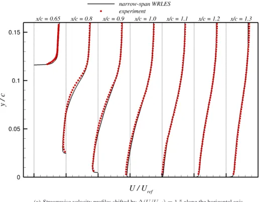
Figures9and10, respectively, plot the mean velocity and Reynolds stress comparisons at a number of streamwise stations. The WRLES profiles are obtained by averaging the unsteady flow in time (over10chord flow times) and along the span. The first station is located atx/c= 0.65, which is just upstream of the separation location. The last station is located atx/c = 1.3, which is downstream of the reattachment location atx/c ≈1.11. The experimental data shown in the comparisons have been obtained using two-dimensional particle image velocimetry (PIV) on the central plane. For clarity, a horizontal shift is applied to the profiles displayed in each subfigure. The respective shift noted for each subfigure denotes the distance between the major ticks on the horizontal axis. These comparisons display good overall agreement between the simulation and experiment. The Reynolds stress profiles in the simulation appear to be more energetic than the experiment at the first comparison station. We note that the attached boundary layer just upstream of separation is rather thin and the experimental PIV measurement is not sufficiently accurate in the near-wall region. These profiles show that flow separation is accompanied by a rapid growth of Reynolds stresses and thickening of the separated shear layer. The separated shear layer expands with streamwise distance and subsequently reattaches on the lower wall.
Although these initial results from the narrow-span WRLES are very encouraging, the calculations performed on a domain with a doubled span predict an earlier reattachment of the separated flow, as will be seen. We discuss the findings from the wide-span calculations next. The observations made from the wide-span WRLES suggest that the seemingly good predictions obtained in the narrow-span WRLES might have been fortuitous.
x / c Cf K -0.5 0 0.5 1 1.5 -0.002 0 0.002 0.004 0.006 0.008 -2E-06 0 2E-06 4E-06 6E-06
experiment (with end plates) narrow-span WRLES relaminarization parameter, K (a) Cfdistribution. x / c Cp -0.5 0 0.5 1 1.5 2 -1 -0.8 -0.6 -0.4 -0.2 0 0.2 0.4
experiment with end plates experiment without end plates narrow-span WRLES
(b)Cpdistribution.
(a) Streamwise velocity profiles shifted by∆(U/Uref) = 1.5along the horizontal axis.
(b) Vertical velocity profiles shifted by∆(V /Uref) = 0.25along the horizontal axis.
(a) Streamwise component profiles shifted by∆(hu′u′i/U2
ref) = 0.1along the horizontal axis.
(b) Vertical component profiles shifted by∆(hv′v′i/U2
ref) = 0.05along the horizontal axis.
(c) Shear component profiles shifted by∆(hu′v′i/U2
ref) = 0.05along the horizontal axis.
2. Wide-Span Calculations
The follow-up calculations performed on a domain with a span of0.4cshow that the separation location in the wide-span WRLES is located atx/c ≈0.661, which is fairly close to the experimentally observed value ofx/c≈0.665. However, the separated flow in the wide-span WRLES is found to reattach earlier than expected. This clearly indicates that the simulation predictions are sensitive to the span chosen in the calculation. Other WMLES studies36, 37 also show a similar trend in which increasing the span moves the reattachment location upstream and the reattachment location settles down with a span of about0.4c. A systematic study regarding the effect of SGS model, tunnel back pressure, upstream boundary layerReθand grid refinement is performed in an attempt to better understand the reason for the early reattachment observed in the wide-span case.
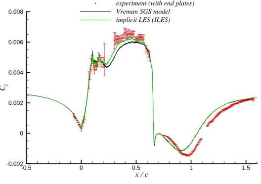
EFFECT OFSGSMODEL: We initially conjectured that the separated shear layer initial conditions might have been affected by the SGS model and this could in turn have affected the spreading rate and the subsequent reattachment location of the separated flow. To explore whether this might indeed be the case, two calculations are performed to study the SGS model effect. The first one employs the static Vreman SGS model32 with a fixed model coefficient
of 0.025. The second calculation is run as implicit LES (ILES), which does not employ any explicit SGS model, but treats the dissipation of the numerical scheme as an implicit SGS model. For both cases, the upstream incoming turbulent boundary layer is generated by adding the recycled turbulent fluctuations to the RANS mean inflow profile, as discussed earlier in sectionIII.B.1. Figure11compares theCfdistributions from the two calculations. Interestingly, the peakCf region prior to flow separation is predicted better by ILES. However, the two predictions are nearly the same everywhere else and the early reattachment location is also nearly identical. Because of its better overallCf prediction, ILES is used in all subsequent calculations.
x / c Cf -0.5 0 0.5 1 1.5 -0.002 0 0.002 0.004 0.006 0.008
experiment (with end plates) Vreman SGS model implicit LES (ILES)
Figure 11. Effect of SGS model onCfdistribution for the wide-span WRLES.
EFFECT OF TUNNEL BACK PRESSURE: The tunnel back pressure in the earlier-referenced RANS studies was set slightly below the upstream reference pressure in an ad hoc manner and the possible back pressure influence on the separation region has not been thoroughly examined. Three calculations are therefore performed to study the effect of tunnel back pressure. There is in fact an additional rationale for this parametric study. In the experiment, the hump model was mounted on a splitter plate, which was then placed some distance above the lower tunnel wall. To control the flow underneath the splitter plate and prevent separation over the leading edge, a flap deflected upward was used at a short distance downstream of the hump trailing edge. To see whether the downstream flow modifications caused
by this flap might have influenced the flow reattachment point, we perform three simulations in which the tunnel back pressure,pb, is respectively set topb/pref = 0.998,0.999and1.001, whereprefis the reference upstream pressure (at x/c = −2.14). For all cases, the upstream incoming turbulent boundary layer is generated by adding the recycled turbulent fluctuations to the RANS mean inflow profile, as discussed in sectionIII.B.1. Figure12(a) shows the Cf comparison between the cases ofpb/pref= 0.998and0.999. According to this figure, the tunnel back pressure does have some effect on the reattachment location, with the slightly lower back pressure creating earlier reattachment than the slightly higher back pressure case. To see whether this trend will continue to hold, we increasepb/prefto1.001 and examine the corresponding comparison withpb/pref= 0.999in Figure12(b). We see that the difference between these two cases is minimal. These findings suggest that the back pressure effect is not strong enough to fully explain the early flow reattachment.
EFFECT OF INCOMING UPSTREAM BOUNDARY LAYER: The possible influence of the upstream turbulent boundary layer conditions on the reattachment location is investigated next. As discussed earlier in sectionIII.B.1, we consider two approaches to define the upstream boundary layer conditions. The first approach matches the reported upstream skin friction in the experiment and hence setsReθ = 5000for the incoming boundary layer upstream of the hump. Available mean velocity and Reynolds stress profiles from the DNS of a canonical flat-plate turbulent boundary layer24
atReθ = 5000are used for the inflow generation technique in the first approach. The second approach, on the other hand, takes the mean velocity profile available from RANS (which matches the reported experimental velocity profile fairly well) and adds the turbulent fluctuations to this mean profile using the inflow generation technique. We note that the skin friction of the RANS profile does not exactly match the reported experimental value. Both cases are run with a back pressure ofpb/pref= 0.999. Figure13shows theCfcomparison between the two inflow conditions. We observe that the first approach creates a slightly higherCf in the region upstream of the hump, which also seems to affect theCf values in the peak region prior to separation. TheCf values in this region are slightly higher in the first approach. Nevertheless, the overall effect on the separated and reattachment regions appears minimal and both inflow conditions cause a nearly identical reattachment point.
EFFECT OF GRID REFINEMENT: The parametric studies conducted so far with regard to the SGS model, back pres-sure and upstream boundary layer conditions reveal relatively minor effects that do not completely explain the early reattachment observed in the wide-span calculation. This observation prompted us to next turn our attention toward a grid refinement study. After an inspection of instantaneous flow structures, we determined that a grid refinement in the wall-normal direction would likely be beneficial both in the attached and separated regions. Hence, in the first step of grid refinement, we increase only the number of grid points in the wall-normal direction both in the attached and separated regions, while keeping the minimum grid spacing on the wall the same as before. By readjusting the grid stretching ratio, we obtain a factor of2to3wall-normal grid refinement both in the attached and separated regions. The refined grid contains about850million points total. The streamwise and spanwise grid spacings in the refined grid are the same as those in the original wide-span grid that has420million points. For both cases, the upstream incoming turbulent boundary layer is again generated by adding the recycled turbulent fluctuations to the RANS mean inflow profile and the back pressure is set topb/pref= 0.999.
Figure 14(a) shows the effect of grid refinement on theCf distribution. We observe that grid refinement has essentially no effect onCf in the attached region but the curve is shifted downstream in the separated flow region, bringing the reattachment location closer to the experiment. However, the predicted reattachment location on the refined grid still falls short of the experimental location. This suggests that another level of grid refinement may be necessary. The effect of grid refinement on theCp distribution is shown in Figure14(b). The primary suction peak remains unaffected by grid refinement, while the secondary peak displays a small downstream shift in accordance with the delayed flow reattachment.
Figures15and16, respectively, plot the mean velocity and Reynolds stress comparisons for the wide-span WRLES on the original and refined grids. The first observation we make from these two figures is that grid refinement in the wall-normal direction does not have a significant impact on the predicted mean velocity profiles and Reynolds stresses at the streamwise locations shown. The mean velocity field predicted on the refined grid does appear to have a slight improvement at some locations. The profiles taken in the attached region just before flow separation (i.e., at
x/c = 0.65) show nearly identical Reynolds stress distributions for the two grids, suggesting that the wall-normal grid refinement was probably unnecessary in the attached region. Nevertheless, the grid refined in the wall-normal direction predicts a later reattachment location, as shown earlier in the skin-friction distribution comparison. These observations lead to the possibility that perhaps the improved grid resolution in the near-wall region of the separation bubble, rather than the improved grid resolution in the separated shear layer region, is responsible for the delayed reattachment. Figure17provides evidence for this possibility. This figure depicts the mean velocity vectors of the
x / c Cf -0.5 0 0.5 1 1.5 -0.002 0 0.002 0.004 0.006 0.008
experiment (with end plates)
back pressure = 0.998*pref : reattachment at x/c = 1.0587 back pressure = 0.999*pref : reattachment at x/c = 1.0646
(a) Comparison betweenpb/pref= 0.998and0.999.
x / c Cf -0.5 0 0.5 1 1.5 -0.002 0 0.002 0.004 0.006 0.008
experiment (with end plates)
back pressure = 0.999*pref : reattachment at x/c = 1.0646 back pressure = 1.001*pref : reattachment at x/c = 1.0625
(b) Comparison betweenpb/pref= 0.999and1.001.
x / c Cf -0.5 0 0.5 1 1.5 -0.002 0 0.002 0.004 0.006 0.008
experiment (with end plates)
RANS inflow velocity profile with recycled fluctuations flat plate Re = 5000 turbulent inflow conditions
Figure 13. Effect of upstream boundary layer onCfdistribution for the wide-span WRLES.
reversed flow region in the vicinity ofx/c= 1. The reversed region of the separation bubble creates a thin boundary layer on the bottom wall. We see that the vector magnitudes on the original grid rise rather rapidly with normal distance from the wall, indicating that the original grid may not have had sufficient resolution to properly resolve this thin boundary layer. The refined grid clearly resolves this region better than the original grid does since it contains a greater number of points in the near-wall region where the vector magnitudes change rapidly. A better resolution of the reversed flow near-wall region may have been the main factor responsible for the later reattachment obtained on the refined grid.
The second observation we make from Figure16is that the wide-span calculations predict considerably higher Reynolds stress levels within the separation bubble, as compared to the predictions of the narrow-span WRLES shown earlier. In particular, the streamwise Reynolds stress levels in the wide-span WRLES are much higher throughout the whole separation bubble. Despite such differences in the Reynolds stress levels, both the narrow-span WRLES and the refined grid wide-span WRLES predict reattachment locations that are quite close (x/c≈1.095versusx/c≈1.091). This is puzzling, as one would expect the wide-span WRLES to be more reliable than the narrow-span WRLES, yet the narrow-span WRLES shows better agreement with the experimental results when it comes to the Reynolds stresses.
There could be a number of factors that contribute to the discrepancy seen in the Reynolds stress predictions. The first factor is the statistical time sample difference between the two cases. The wide-span case was time-averaged over30chord flow times while the narrow-span case was averaged over10chord flow times. A longer time average might affect the narrow-span WRLES Reynolds stresses to some degree, but any possible shift in the Reynolds stresses resulting from a longer time sample is unlikely to be as dramatic as the considerably higher levels seen in the wide-span case. The second factor is the Mach number mismatch between the two cases. As mentioned earlier, the Mach number was increased to0.2for the wide-span case to speed up the calculations. The possible Mach number effect will be further investigated in future work. On a related note, Li et al.38 recently performed simulations of the flow
over a backward-facing step at Mach numbers of0.2,0.3and0.4, and found that the Mach number increase in the given range causes a faster downward bending of the separated shear layer, thus leading to an earlier reattachment. The planned simulation at Mach0.1will help determine whether our problem displays a similar behavior between the Mach numbers of0.1and0.2. The simulation at Mach0.1will also examine the effect of statistical sample size on the Reynolds stresses in more detail. Differences in upstream conditions between the simulation and experiment may be the third contributing factor to the Reynolds stress discrepancy. Unfortunately, there are no detailed experimental measurements taken in the attached region well upstream of the separated region, and hence we cannot judge how
x / c Cf -0.5 0 0.5 1 1.5 -0.002 0 0.002 0.004 0.006 0.008
experiment (with end plates) original grid refined grid (a)Cfdistributions. x / c Cp -0.5 0 0.5 1 1.5 2 -1 -0.8 -0.6 -0.4 -0.2 0 0.2 0.4
experiment with end plates experiment without end plates original grid
refined grid
(b)Cpdistributions.
(a) Streamwise velocity profiles shifted by∆(U/Uref) = 1.5along the horizontal axis.
(b) Vertical velocity profiles shifted by∆(V /Uref) = 0.25along the horizontal axis.
Figure 15. Mean flow velocity comparisons for the wide-span WRLES on the original and refined grids. Symbols denote the experimental measurement.
(a) Streamwise component profiles shifted by∆(hu′u′i/U2
ref) = 0.1along the horizontal axis.
(b) Vertical component profiles shifted by∆(hv′v′i/U2
ref) = 0.05along the horizontal axis.
(c) Shear component profiles shifted by∆(hu′v′i/U2
ref) = 0.05along the horizontal axis.
well the simulation and experiment agree in that region. Missing end-plate effects in the simulation might be another contributing factor. To reiterate, the distance between the end plates in the experiment is1.4c. We are not clear on whether the experimental span is wide enough for the end plates not to influence the statistical data measured on the central plane. A repeat of this benchmark experiment with and without end plates (and perhaps with different spans) that can provide additional detailed measurements both in the attached and separated regions would be very useful for future computational investigations and help us better understand the end-plate effects.
Despite the Reynolds stress discrepancy, the skin-friction curve predicted in the refined wide-span WRLES shows reasonable overall agreement with the experiment. The separation-bubble length measured in the experiment is0.445c. The best result from the wide-span WRLES predicts the separation-bubble length as0.43c. This translates to an error of about3.4%in the separation-bubble length relative to the experimental observation.
The fact that the narrow-span WRLES predicts a longer reattachment length than the doubled span case (i.e., original wide-span WRLES performed on 420 million points) suggests two likely sources of numerical error and possible error cancellation at play in the narrow-span WRLES. The first error originates from the narrow span, which might have constrained the growth of large-scale structures in the separated shear layer. This would in turn influence the spreading rate of the shear layer and the reattachment location. Doubling the span reduces this constraint on the growth of large structures, causing the separated flow to grow faster and reattach earlier in the original wide-span WRLES. Grid refinement in the wall-normal direction is found to improve the reattachment location prediction of the wide-span WRLES. This means that the wall-normal resolution in the separated region of the narrow-span WRLES was also insufficient, because the narrow-span WRLES has the same grid resolution as the original wide-span WRLES. Our observations therefore suggest that these two main errors (insufficient span and insufficient grid resolution) might have canceled each other and fortuitously produced good predictions in the narrow-span WRLES.
x / c y / c 0.9985 0.999 0.9995 1 1.0005 0 0.0002 0.0004 0.0006 0.0008 0.001 0.0012 0.0014 original grid refined grid
Figure 17. Mean flowfield velocity vectors of the reversed region in the vicinity ofx/c= 1.
IV.
Conclusions
A number of wall-resolved simulations have been performed in this study for the NASA wall-mounted hump problem, which has proven to be a challenging benchmark case for the numerous turbulence simulations. The best result from the wide-span WRLES shows a difference of about3.4%in the separation-bubble length relative to the experiment. The current simulations also provide good overall prediction of the skin-friction curve, including the relaminarization observed over the front section of the hump. This relaminarization region was not captured in the
earlier studies of the problem by other researchers.
A systematic study regarding the effect of domain span, SGS model, tunnel back pressure, upstream boundary layerReθand grid refinement is performed. The separation-bubble length is found to be sensitive to the span of the domain. The problems that emerged during the course of this work are discussed and viable solutions are presented. The comparison between a calculation done with the Vreman SGS model and another one performed as ILES shows that the SGS model mainly affects the peak skin-friction region prior to flow separation, but does not alter the reat-tachment location. ILES predicts the peak skin-friction region better than Vreman SGS model does. The details of the upstream incoming turbulent boundary layer determine the skin friction upstream of the hump, which then influences the peak skin-friction levels prior to separation. The two different upstream boundary layer conditions cause a similar reattachment point. The tunnel back pressure has a small effect on the reattachment location. The more significant change in the predicted reattachment location in the wide-span WRLES is seen after grid refinement in the wall-normal direction. Evidence shows that the improved grid resolution in the near-wall region of the separation bubble, rather than the improved grid resolution in the separated shear layer region, might be responsible for the later reattachment.
Although the Reynolds stress predictions within the separation bubble are found to be in better agreement with the experiment in the narrow-span WRLES, the findings suggest that numerical errors from different sources might have canceled each other and fortuitously produced good predictions. Despite850million grid points used in the largest wide-span WRLES, some differences between the predictions and experimental observations still exist. The possible Mach number effect on the Reynolds stresses predicted by the wide-span WRLES and the effect of additional grid refinement in the near-wall region of the separation bubble warrant further investigation. The potentially significant end-plate effects in the experiment also need to be investigated further. Our experience and observations in this study reaffirm the daunting challenges associated with the prediction of high Reynolds number separated flows. A repeat of this benchmark experiment with and without end plates (and perhaps with different spans) that can provide additional detailed measurements both in the attached and separated regions would be very useful for future computational investigations and help us better understand the end-plate effects.
Acknowledgments
The work of the first author was sponsored by the NASA Transformational Tools and Technologies Project un-der the cooperative agreement NNL09AA00A. The simulations used the computing resources provided by the NASA High-End Computing (HEC) Program through the NASA Advanced Supercomputing (NAS) Division at Ames Re-search Center. The authors thank Drs. Gary Coleman and Steve Woodruff for their review and helpful comments on an earlier version of the manuscript.
References
1Rumsey, C. L., Gatski, T. B., Sellers III, W. L., Vasta, V. N., and Viken, S. A., “Summary of the 2004 Computational Fluid Dynamics
Validation Workshop on Synthetic Jets,” AIAA Journal, Vol. 44, No. 2, 2006, pp. 194–207.
2Greenblatt, D., Paschal, K. B., Yao, C.-S., Harris, J., Schaeffler, N. W., and Washburn, A. E., “A Separation Control CFD Validation Test
Case, Part 1: Baseline and Steady Suction,” AIAA Journal, Vol. 44, No. 12, 2006, pp. 2820–2830.
3Avdis, A., Lardeau, S., and Leschziner, M., “Large Eddy Simulation of Separated Flow over a Two-Dimensional Hump with and without
Control by Means of a Synthetic Slot-Jet,” Flow, Turbulence and Combustion, Vol. 83, No. 3, 2009, pp. 343–370.
4
Shur, M. L., Spalart, P. R., Strelets, M. K., and Travin, A. K., “Synthetic Turbulence Generators for RANS-LES Interfaces in Zonal Simulations of Aerodynamic and Aeroacoustic Problems,” Flow, Turbulence and Combustion, Vol. 93, No. 1, 2014, pp. 63–92.
5Park, G. I., “Wall-Modeled LES in Unstructured Grids: Application to the NASA Wall-Mounted Hump,” AIAA Paper 2016-1560,
54th
AIAA Aerospace Sciences Meeting, San Diego, CA, January 2016.
6Duda, B. and Fares, E., “Application of a Lattice-Boltzmann Method to the Separated Flow Behind the NASA Hump,” AIAA Paper
2016-1836,54thAIAA Aerospace Sciences Meeting, San Diego, CA, January 2016.
7Iyer, P. S. and Malik, M. R., “Wall-Modeled Large Eddy Simulation of Flow Over a Wall-Mounted Hump,” AIAA Paper 2016-3186,46th
AIAA Fluid Dynamics Conference, Washington, DC, June 2016.
8You, D., Wang, M., and Moin, P., “Large-Eddy Simulation of Flow over a Wall-Mounted Hump with Separation Control,” AIAA Journal,
Vol. 44, No. 11, 2006, pp. 2571–2577.
9Franck, J. A. and Colonius, T., “Compressible Large-Eddy Simulation of Separation Control on a Wall-Mounted Hump,” AIAA Journal,
Vol. 48, No. 6, 2010, pp. 1098–1107.
10Postl, D. and Fasel, H. F., “Direct Numerical Simulation of Turbulent Flow Separation from a Wall-Mounted Hump,” AIAA Journal, Vol. 44,
No. 2, 2006, pp. 263–272.
11Yeh, C.-A., Munday, P. M., Taira, K., and Munson, M. J., “Drag Reduction Control for Flow over a Hump with Surface-Mounted
Thermoa-coustic Actuator,” AIAA Paper 2015-0826,53rdAIAA Aerospace Sciences Meeting, Kissimmee, FL, January 2015.
12Ashcroft, G. and Zhang, X., “Optimized Prefactored Compact Schemes,” Journal of Computational Physics, Vol. 190, No. 2, 2003, pp. 459–
13Lele, S. K., “Compact Finite Difference Schemes with Spectral-like Resolution,” Journal of Computational Physics, Vol. 103, No. 1, 1992,
pp. 16–42.
14Gaitonde, D. V. and Visbal, M. R., “Pad´e-Type Higher-Order Boundary Filters for the Navier-Stokes Equations,” AIAA Journal, Vol. 38,
No. 11, 2000, pp. 2103–2112.
15
Visbal, M. R. and Gaitonde, D. V., “Very High-Order Spatially Implicit Schemes for Computational Acoustics on Curvilinear Meshes,”
Journal of Computational Acoustics, Vol. 9, No. 4, 2001, pp. 1259–1286.
16Sherer, S. E. and Scott, J. N., “High-Order Compact Finite-Difference Methods on General Overset Grids,” Journal of Computational Physics, Vol. 210, No. 2, 2005, pp. 459–496.
17Ekaterinaris, J. A., “Implicit, High-Resolution, Compact Schemes for Gas Dynamics and Aeroacoustics,” Journal of Computational Physics,
Vol. 156, No. 2, 1999, pp. 272–299.
18Uzun, A., Hussaini, M. Y., and Streett, C. L., “Large-Eddy Simulation of a Wing Tip Vortex on Overset Grids,” AIAA Journal, Vol. 44, No. 6,
2006, pp. 1229–1242.
19Uzun, A. and Hussaini, M. Y., “Investigation of High Frequency Noise Generation in the Near-Nozzle Region of a Jet Using Large Eddy
Simulation,” Theoretical and Computational Fluid Dynamics, Vol. 21, No. 4, 2007, pp. 291–321.
20Uzun, A. and Hussaini, M. Y., “Simulation of Noise Generation in Near-Nozzle Region of a Chevron Nozzle Jet,” AIAA Journal, Vol. 47,
No. 8, 2009, pp. 1793–1810.
21Uzun, A. and Hussaini, M. Y., “Prediction of Noise Generated by a Round Nozzle Jet Flow Using Computational Aeroacoustics,” Journal of Computational Acoustics, Vol. 19, No. 3, 2011, pp. 291–316.
22Uzun, A. and Hussaini, M. Y., “Simulations of Vortex Formation Around a Blunt Wing Tip,” AIAA Journal, Vol. 48, No. 6, 2010, pp. 1221–
1234.
23Uzun, A. and Hussaini, M. Y., “An Application of Delayed Detached Eddy Simulation to Tandem Cylinder Flow Field Prediction,” Comput-ers & Fluids, Vol. 60, 2012, pp. 71–85.
24
Sillero, J. A., Jim´enez, J., and Moser, R. D., “One-Point Statistics for Turbulent Wall-Bounded Flows at Reynolds numbers up toδ+ ≈
2000,” Physics of Fluids, Vol. 25, 2013, pp. 105102.
25Eitel-Amor, G., ¨Orl¨u, R., and Schlatter, P., “Simulation and Validation of a Spatially Evolving Turbulent Boundary Layer up to Reθ =
8300,” International Journal of Heat and Fluid Flow, Vol. 47, 2014, pp. 57–69.
26Rumsey, C. L., Private Communication, February 2016.
27Naughton, J. W., Viken, S. A., and Greenblatt, D., “Skin-Friction Measurements on the NASA Hump Model,” AIAA Journal, Vol. 44, No. 6,
2006, pp. 1255–1265.
28Uzun, A. and Hussaini, M. Y., “Some Issues in Large-Eddy Simulations for Chevron Nozzle Jet Flows,” Journal of Propulsion and Power,
Vol. 28, No. 2, 2012, pp. 246–258.
29Morgan, B., Larsson, J., Kawai, S., and Lele, S. K., “Improving Low-Frequency Characteristics of Recycling/Rescaling Inflow Turbulence
Generation,” AIAA Journal, Vol. 49, No. 3, 2011, pp. 582–597.
30Ikeda, T., Atobe, T., Konishi, Y., Nagai, H., and Asai, K., “Numerical Study of Wind-Tunnel Acoustic Resonance Induced by
Two-Dimensional Airfoil Flow at Low Reynolds Number,”29thCongress of the International Council of the Aeronautical Sciences, St. Petersburg,
Russia, September 2014.
31Pirozzoli, S. and Colonius, T., “Generalized Characteristic Relaxation Boundary Conditions for Unsteady Compressible Flow Simulations,” Journal of Computational Physics, Vol. 248, 2013, pp. 109–126.
32Vreman, A. W., “An Eddy-Viscosity Subgrid-Scale Model for Turbulent Shear Flow: Algebraic Theory and Applications,” Physics of Fluids,
Vol. 16, No. 10, 2004, pp. 3670–3681.
33
Hunt, J. C. R., Wray, A. A., and Moin, P., “Eddies, Stream, and Convergence Zones in Turbulent Flows,” Center for Turbulence Research Report CTR-S88, 1988.
34Bourassa, C., An Experimental Investigation of an Accelerated Turbulent Boundary Layer, Ph.D. thesis, University of Notre Dame, Notre
Dame, IN, 2005.
35Narasimha, R. and Sreenivasan, K. R., “Relaminarization in Highly Accelerated Turbulent Boundary Layers,” Journal of Fluid Mechanics,
Vol. 61, 1973, pp. 417–447.
36Strelets, M. K. and Spalart, P. R., Private Communication, April 2016. 37Iyer, P. S., Private Communication, May 2016.
38
Li, D., Komperda, J., Ghiasi, Z., and Mashayek, F., “The Effect of Inflow Mach Number on the Reattachment in Subsonic Flow over a Backward-Facing Step,” AIAA Paper 2016-2077,54thAIAA Aerospace Sciences Meeting, San Diego, CA, January 2016.