www.ssoar.info
Implied rates of return, the discount rate effect, and
market risk premia
Breuer, Wolfgang; Gürtler, Marc
Arbeitspapier / working paper
Zur Verfügung gestellt in Kooperation mit / provided in cooperation with: SSG Sozialwissenschaften, USB Köln
Empfohlene Zitierung / Suggested Citation:
Breuer, W., & Gürtler, M. (2010). Implied rates of return, the discount rate effect, and market risk premia.
(IF Working Paper Series, IF33V3/10). Braunschweig: Technische Universität Braunschweig, Department Wirtschaftswissenschaften, Institut für Finanzwirtschaft. https://hdl.handle.net/10419/55241
Nutzungsbedingungen:
Dieser Text wird unter einer Deposit-Lizenz (Keine Weiterverbreitung - keine Bearbeitung) zur Verfügung gestellt. Gewährt wird ein nicht exklusives, nicht übertragbares, persönliches und beschränktes Recht auf Nutzung dieses Dokuments. Dieses Dokument ist ausschließlich für den persönlichen, nicht-kommerziellen Gebrauch bestimmt. Auf sämtlichen Kopien dieses Dokuments müssen alle Urheberrechtshinweise und sonstigen Hinweise auf gesetzlichen Schutz beibehalten werden. Sie dürfen dieses Dokument nicht in irgendeiner Weise abändern, noch dürfen Sie dieses Dokument für öffentliche oder kommerzielle Zwecke vervielfältigen, öffentlich ausstellen, aufführen, vertreiben oder anderweitig nutzen.
Mit der Verwendung dieses Dokuments erkennen Sie die Nutzungsbedingungen an.
Terms of use:
This document is made available under Deposit Licence (No Redistribution - no modifications). We grant a exclusive, non-transferable, individual and limited right to using this document. This document is solely intended for your personal, non-commercial use. All of the copies of this documents must retain all copyright information and other information regarding legal protection. You are not allowed to alter this document in any way, to copy it for public or commercial purposes, to exhibit the document in public, to perform, distribute or otherwise use the document in public.
By using this particular document, you accept the above-stated conditions of use.
Working Paper Series
Implied Rates of Return, the Discount Rate Effect,
and Market Risk Premia
by Wolfgang Breuer and Marc Gürtler
No.: IF33V3/10
First Draft: 2010-02-11 This Version: 2010-10-22
University of Braunschweig – Institute of Technology Department of Finance
Abt-Jerusalem-Str. 7 38106 Braunschweig
Implied Rates of Return, the Discount Rate Effect,
and Market Risk Premia
by Wolfgang Breuer
*and Marc Gürtler
**Abstract. We show analytically under quite general conditions that implied rates of return based on analysts’ earnings forecasts are only a downward biased estimator for future expected one-period returns and therefore not suited for computing market risk premia. The extent of this bias is substantial as verified by a bootstrap approach. We present an alternative estimation equation for future expected one-period returns based on current and past implied rates of return that is superior to simple estima-tors based on historical returns. The reason for this superiority is a lower variance of estimation results and not the circumvention of the discount rate effect typically stated as a major problem of estimators based on historical return realizations. The superiority of this new approach for portfolio selection pur-poses is verified numerically for our bootstrap environment and empirically for real capital market data. Keywords: analysts’ earnings forecasts, discount rate effect, equity premium puzzle, implied rate of
return
JEL classification: G11, G12, G14
* Professor Dr. Wolfgang Breuer
RWTH Aachen University Department of Finance Templergraben 64 52056 Aachen Germany Fon: +49 241 8093539 Fax: +49 241 8092163 E-mail: wolfgang.breuer@rwth-aachen.de
** Professor Dr. Marc Gürtler
Braunschweig Institute of Technology Department of Finance Abt-Jerusalem-Str. 7 38106 Braunschweig Germany Fon: +49 531 3912895 Fax: +49 531 3912899 E-mail: marc.guertler@tu-bs.de
1 1 Introduction
There is a long and on-going debate regarding the precise value of the market risk premium, i.e. the difference between the expected one-period return of a broad portfolio of stocks and the corresponding risk-free interest rate. In particular, according to the seminal paper by Mehra and Prescott (1985), theoretically justifiable market risk premia are much smaller than those computed on the basis of averages of historical stock returns. Several avenues have been taken to address this issue. First of all, one may improve upon the theoretical analysis in order to explain higher risk premia than determined by Mehra and Prescott (1985). Such an approach is followed by Benartzi and Thaler (1995) and Barberis et al. (2001) who make use of behavioral finance arguments like myopia, loss aversion, and ambiguity aversion in order to resolve the “equity premium puzzle”. Nevertheless, such approaches face some problems: Even if there might be behavioral anomalies due to bounded rationality so that stock investments are not sufficiently appreciated why do investors not take measures in order to mitigate the consequences of their bounded rationality as Ulysses had done when tying himself to the mast just to save himself against the Sirens (see DeLong and Magin, 2009, p. 200)? Other theoretical explanations refer to transaction costs arguments (see, e.g., Mankiw and Zeldes, 1991, Constantinides et al., 2002) or (temporary) subjective misperceptions of return distributions (see, e.g., McGrattan and Prescott, 1993, and Fama and French, 2002), but – at least up to now – are not fully convincing.
Therefore, a second strand of literature has gained more and more importance, i.e., alternative ways to estimate market risk premia. First of all, one may refine computations based on historical return data as in Fama and French (2002). Secondly, one may simply make use of survey data extracted by asking specialists directly for their opinion regarding market risk premia (see, e.g., Welch, 2000, and Graham and Campbell, 2007). Certainly, the procedures by which those experts have obtained their market risk premium estimates remain opaque.
2 Thirdly, as a quite new approach, one may make use of credit risk spread data in order to derive equity risk premia on an options-price theoretical basis (see, e.g., Berg and Kaserer, 2008). Fourthly and finally, one may rely on analysts’ earnings forecasts as the basis of net present value computations (see, e.g., Claus and Thomas, 2001, and Gebhardt et al., 2001). Equaling these net present values with current stock prices makes it possible to derive an internal or implied rate of return that may be used as an estimator for future expected one-period returns. After subtraction of the relevant riskless interest rate, this gives an estimator for the market risk premium. As implied rates of return are generally smaller than the historical average of realized rates of return, this alternative estimation procedure also may contribute to resolving (or at least mitigating) the equity premium puzzle (see, e.g. Claus and Thomas, 2001).
Thereby, referring to implied rates of return instead of estimators based on historical rates of return may be superior because the so-called discount rate effect (first discussed by Fama and French, 1988) is effectively avoided. Changes in relevant discount rates, i.e. implied rates of return, are ceteris paribus associated with opposing reactions of stock prices. Assume, for example, an increase in the implied rate of return from 5 % to 10 % for a situation with a constant expected dividend of $1 per period till infinity. Then the stock price will fall from $20 to $10 implying an immediate negative return of (1−10)/20 = −45 %, while an investor will earn on average 1/10 = 10 % per period on this stock after this discount rate adjustment instead of 1/20 = 5 % in the situation before this change. Apparently, estimators based on historical return realizations have to cope with the problem of the discount rate effect. Large lengths of historical samples are necessary to neutralize outliers like those −45 %, but then stationarity assumptions may not hold any longer. On the contrary, the estimation approach based on implied rates of return will immediately reveal the change in expected rates of return
3 from 5 % to 10 %. For dividend forecasts being sufficiently precise, this estimation procedure thus seems to be advantageous to approaches that rely on historical return realizations.
Apparently, utilizing implied rates of return in this sense at least implicitly assumes that analysts’ earnings forecasts are suited to derive representative return expectations for the whole capital market. In what follows, we do not address primarily this problem of analysts’ expectations being representative for the capital market as a whole, but we ask whether these forecasts can be exploited to derive reasonable estimators of expected rates of return regardless of their representativeness: However, in a somewhat indirect manner, our findings are relevant for this latter issue as well, as we will explain later on.
To be more precise, we show analytically and numerically that implied rates of return per se are only loosely connected to expected one-period stock returns. In fact, both rates of return are systematically identical only in the special case of implied rates of returns being constant over time. In case implied rates of return are varying randomly, even in situations with an expected change of zero from period to period, expected one-period stock returns are higher than those implied rates of return. Certainly, this bias is the greater the more implied rates of return are fluctuating over time. Nevertheless, it might be that the empirical relevance of this bias problem only is rather small. However, we show that in spite of only a small variation in implied rates of return over time, the resulting bias may be quite large. We present a bootstrap approach with a difference between implied rates of return and true expected rates of return of about 1 percentage point on a monthly (!) basis and interpret this as evidence for implied rates of return being only poor predictors of expected one-period returns. This holds true, although in our settings implied rates of return are indeed the true discount rates for future earnings, as future expected dividends are – by assumption – forecast without any bias.
4 As is long known in financial literature, as a consequence of Jensen’s inequality, discount rates and average historical one-period returns cannot be identical in situations under risk. In fact, the arithmetic mean of historical return realizations is only an upward biased estimator for the implied rate of return and thus the adequate discount rate in net present value computations (see, e.g., Butler and Schachter, 1989). In a similar way, we now show that the implied rate of return as a discount rate is only a downward biased estimator of expected one-period returns. Our paper therefore is related to the literature that addresses the problem of upward biases in arithmetic mean estimators like Butler and Schachter (1989), Cooper (1996) and – more recently – Breuer et al. (2010).
Moreover, we are able to mitigate this estimation problem with respect to current implied rates of return by deriving an unbiased forecast equation regarding future expected one-period returns which refers to current and historical implied rates of return and which may be utilized as a basis for predicting future one-period returns. Compared to determining future expected rates of return on the basis of historical return realizations, it offers the advantage of not depending on dividend volatility. Estimators based on implied rates of return may thus be advantageous not primarily because they offer shelter against the discount rate effect, but because they prevent estimates from being affected by dividend fluctuations. This is even true in situations where implied rates of return are expected to be constant once again after changes caused by exogenous shocks. In such a situation, the new implied rate of return would indeed be an unbiased estimator of future expected one-period returns. This, however, would also be true with respect to any future return realization. In this sense, the discount rate effect does not really lead to a significant advantage of estimates based on implied rates of return in comparison to estimates based on historical return realizations. But once again, the variance of estimators would be higher in the latter case due to the adverse influence of dividend volatility.
5 There are two main implications of our theoretical findings: First of all, one may not refer to considerations of current implied rates of return as an estimator for expected rates of return in order to resolve the equity premium puzzle because these estimators are downward biased. Moreover, our newly introduced unbiased estimator of expected rates of return that refers to past and current implied rates of return will – on average – lead to the same estimates of market risk premia as an estimator based on historical return realizations. It thus seems that estimators based on implied rates of return cannot contribute to the resolution of the equity premium puzzle.
Secondly, however, our newly introduced estimator for expected rates of return should do better than an estimator based on historical return realizations in portfolio selection problems from the point of view of an expected utility maximizing investor. We show this analytically and determine the potential extent of the welfare increase by way of our bootstrap approach as well. Nevertheless, biases in analysts’ forecasts (see, e.g., Stickel, 1990, Easterwood and Nutt, 1999 and Capstaff et al., 2001) may affect in practice the success of estimation procedures based on implied rates of return. Therefore, we also present a simple practical application of our approach for real-life capital market data which only consists of combining a given portfolio of risky assets with a riskless security. We find evidence that superior portfolio selection decisions are indeed achievable by the estimation procedure suggested in this paper. In addition, this finding might be interpreted as additional evidence against using implied rates of return as a starting point for estimates of market risk premia, as the latter have to be based on representative expectations that are not suited to result in superior portfolio selection. This view is supported by the fact that estimates of expected rates of return according to our approach are often even negative – a fact which explains their good performance under bearish market conditions, but is not consistent to market expectations. In
6 any case, it may pay to take a closer look at our approach in future research. This holds particular true as our approach may also be utilized in more complex selectivity problems.
The rest of the paper is organized as follows. Section 2 is devoted to an analytical examination of the general bias problem when relying only on current implied rates of return for estimation issues and the derivation of our alternative estimation procedure for future expected one-period returns based on current and past implied rates of return. Additionally, we present the advantage of our approach by the analysis of the simple portfolio selection problem where an investor only has to determine the optimal combination of a risky and a riskless asset. In Section 3, we undertake a bootstrap approach based on data from the German stock market in order to estimate the extent of the bias problem and to determine the welfare gain for investors when referring to our modified approach instead of simple estimates based on actually realized historical returns. We find that – at least for our setting – implied rates of return are not suited as estimators for one-period expected stock returns even if analysts’ forecasts are unbiased. However, our alternative estimation procedure performs far better. Therefore, in Section 4, we take a closer look at our alternative approach for real-life capital market data and investigate its superior performance when compared to estimates of expected rates of return based on historical return realizations. Section 5 concludes.
2 The general bias problem with implied rates of return
At each point in time t we assume the validity of the (single-stage) dividend discount model.
Concretely, we consider a firm that earns (as seen from time t) uncertain dividends d at (discrete) points in time ≥ t+1. Furthermore, the (conditional) expected dividend
t t 1 t 1 t
7 dividend forecasts. The following expected dividends E (d )t ( t+2) are assumed to
increase with an exogenously given constant growth rate g. Summarized, we get
t
t 1 t t 1 t t 1
E (d ) (1 g) E (d ) ⇒ E (d ) (1 g) E (d ) for all t 0 and all t 1. (1) In addition, there shall be just one share of this firm and its (already realized) value amounts
to Vt at time t. Then the implied rate of return rt(impl) as seen from time t is implicitly defined
by the following equation:
(impl) t t 1 t t 1 t (impl) t t t E (d ) E (d ) V r g. r g V (2)
Supporters of the implied rate of returns approach assert that (impl) t
r is a reasonable estimator
for the expected one-period rate of return from holding the stock from time t to time t+1. However, the latter is defined as the expectation value of
t 1 t 1 t 1 t V d r 1. V (3) With t 1 t 2 t 1 (impl) t 1 E (d ) V r g (4) (3) becomes t 1 t 2 t 1 (impl) t 1 t 1 t t 1 (impl) t E (d ) d r g r 1. E (d ) r g (5)
In the following, we make the reasonable assumption of (impl) t 1
r
and E (dt 1 t 2) being independent. We will briefly return to this point later on. In addition, we assume “time
consistency” in dividend expectations, i.e. E (E (d )) E (d )t t 1 t 2 t t 2 . On this basis taking
8 t t 2 t (impl) t t 1 t 1 (impl) t t 1 t t (impl) t 1 t t 1 (impl) t 1 E (d ) E E (d ) r g 1 g E (r ) 1 (r g) E 1 1, r g E (d ) r g ⎛ ⎞ ⎜ ⎟ ⎛ ⎛ ⎞ ⎞ ⎝ ⎠ ⎜ ⎟ ⎜ ⎟ ⎜ ⎝ ⎠ ⎟ ⎝ ⎠ (6) where (impl) t t 1 t 1 t t
E (r ) : E(r | r ,d ) and (impl) 1 (impl) 1 (impl)
t t 1 t 1 t t
E ((r g) ) : E((r g) | r ,d ) stand for
the conditional expectation values given (impl) (impl)
t t
r r
and dt dt. Apparently, for
(impl) (impl) t 1 t r r , (6) simplifies to (impl) t t 1 t E (r ) r . (7)
In such a situation, estimating expected returns simply by looking at (impl) t
r obviously is
superior to any approach that is based on the consideration of historical return realizations, as the variance of this unbiased estimator is just zero. However, in the general case, (7) will not hold true. According to Jensen’s inequality, the following relationship is valid:
t (impl) (impl) t 1 t t 1 1 1 E . r g E (r ) g ⎛ ⎞ ⎜ ⎟ ⎝ ⎠ (8)
As a consequence, for (impl) t 1
r and E (dt 1 t 2) being independent (or negatively correlated), we have (impl) t t 1 t (impl) t t 1 1 g E (r ) (r g) 1 1. E (r ) g ⎛ ⎞ ⎜ ⎟ ⎝ ⎠ (9)
For the simple case (impl) (impl)
t t 1 t
E (r ) r , i.e. the time series of the implied rates of return
following a martingale, we directly get from (9)
(impl)
t t 1 t
E (r ) r . (10)
The consequences of variations in annual growth rates for the goodness of the implied rate of return as an estimator for the actual expected one-period return can be examined under two different conditions. First of all, one may assume ceteris paribus variations of g by the estimating individual without any direct relevance for market assumptions. This means that
9 we have to distinguish between g(E) and g(M) with the former growth rate being assumed by the estimating individual and the latter being assumed by the market, i.e. entering firm
valuation. Apparently, as long as g(E) < g(M), a rise in g(E) will improve the goodness of (impl) t
r
as an estimator for the true expected one-period return. The reason simply is that variations of
g(E) from g(E) to g(E)+ g(E) do not affect E (r )t t 1 according to (3) but only imply (impl) t
r to rise to
(impl) (E)
t
r g . Since even for g(E) = g(M) the implied rate of return is a downward biased
estimator, this holds true for all growth rates g(E) < g(M) as well. However, it would be advantageous to overestimate g, i.e. to have g(E) > g(M) just in order to reduce the bias problem. Unfortunately, as the extent of the bias is not known, this finding is not really of immediate practical value.
Secondly, one may assume variations of g in situations with g = g(E) = g(M). In this case, based on (6), some comparative statics apply which are presented as part (ii) of the following proposition. Moreover, part (iii) examines the consequences of varying volatility of implied rates of return, while part (i) simply restates our finding according to formula (9).
Proposition 1. Assume the time series of implied rates of return to follow a martingale, i.e. ( impl ) ( impl )
t t 1 t
E ( r ) r for all t, and all implied rates of return and future dividend expectations to be independent. Furthermore, expectations fulfill the “time consistency property”
1 2
( ( ))
t t t
E E d E dt(t 2). Then the following statements apply:
(i) Only for ( impl ) t t 1
Var ( r ) 0, the implied rate of return at time t is an unbiased estimator of the expected rate of return E ( r )t t 1 . Otherwise, we have ( impl )
t t 1 t
10
(ii) The bias in utilizing implied rates of return as an estimator for one-period expected stock returns becomes greater for ceteris paribus greater growth rates g, i.e. the partial derivative
( impl )
t t 1 t
( E ( r ) r ) / g is positive. (iii) Let the implied rate ( impl ,B )
t 1 r
be a mean preserving spread of the implied rate ( impl ,A ) t 1 r , i.e. ( impl ,B ) ( impl ,A ) t 1 t 1 r r with ( impl ,A ) t t 1
E ( | r ) 0 for all realizations ( impl ,A ) t 1
r . In this situation, the estimation bias for B is higher than the bias for A, i.e. ( A ) ( impl ,A ) ( B ) ( impl ,B )
t t 1 t t t 1 t
E ( r ) r E ( r ) r .
Proof.For part (i), see derivation above, for parts (ii) and (iii), see Appendix 1.
Proposition 1 requires that future implied rates of return and expected dividend expectations are independent. From an economic point of view, there is no reason why future implied rates of return and expected dividends should be correlated. A ceteris paribus increase in expected future dividends should lead to a corresponding rise in stock price with the implied rate of return being unaffected. Changes of implied rates of return should be in the first place a consequence of changes in attitudes towards risk, as is a result of the well-known Capital Asset Pricing Model. Therefore, such changes would simply lead to reduced market values with expected future dividends being unaltered. Summarizing, in situations with unbounded rationality we would expect that there is no relationship between future implied rates of return and expected future dividends.
However, things may change if we take into account that the computation of implied rates of return are based on analysts’ dividend forecasts. If these forecasts were independent of actual market forecasts, then changes in analysts’ dividend forecasts would not be compensated by corresponding changes in stock prices. As a consequence, estimators for implied rates of return and future expected dividends would become positively correlated. However, at the same time, the „true“ implied rate of return could only be estimated with a bias, unless market
11 expectations are on average identical to analysts’ expectations. In fact, with a superscript “(A)” for variables based on analysts’ forecasts and “(M)” for variables based on market forecasts, we have:
(A) (M) (M)
(impl,M) (impl,A)
t t 1 t t 1 t t 1
t (impl,A) t (impl,M) t t (A)
t t t t 1 E (d ) E (d ) E (d ) V , V r (r g) g. r g r g ⇒ E (d ) (11)
This gives us the following proposition.
Proposition 2. Assume analysts’ dividend forecasts to be more optimistic than market expectations underlying stock price formation, i.e. ( A ) ( M )
t t 1 t t 1
E ( d ) E ( d ), then the corres-ponding implied rate of return estimator ( impl ,A )
t
r is greater than the corresponding estimator ( impl ,M )
t
r based on market expectations. For given expectations, the difference between ( impl ,A ) t r and ( impl ,M )
t
r is independent of the assumed annual growth rate g of annual cash flows. Proof.See Appendix 2.
In fact, there is empirical evidence that analysts’ earnings forecasts are typically too optimistic (see, e.g., Stickel, 1990, Easterwood and Nutt, 1999 and Capstaff et al., 2001).
Thus, when relying on (impl,A) t
r instead of (impl,M) t
r the corresponding upward bias may (at least)
partially neutralize the downward bias according to formula (10). Nevertheless, it does not seem to be too sensible to fight one estimation error by another. We will return to this issue later on.
Up to now, we have focused on the simple case of the time series of implied rates of return following a martingale. However, an alternative assumption would be to consider implied rates of return that are independently and identically distributed (i.i.d., henceforth) over time. This directly implies
12
(impl) (impl)
t t 1
E (r ) µ for all t. (12)
Apparently, (12) can be viewed as an alternative extension of the “deterministic” case
(impl) (impl)
t 1 t
r r ,
as the latter equality would once again be true in expectation values. Even
under (12), the previous analyses are of use as they show that even for situations with the actual implied rate of return being identical to the expected implied rate of return, the expected one-period return will be greater than the current implied rate of return. All results so far apply to this special case as well. Moreover, it is immediately clear that for current implied rates below the corresponding expectation value the bias will be even greater.
Certainly, by (pure) chance there may also be levels of (impl) t
r
above µ(impl) so that the
expected one-period return is forecast without any bias. However, if we compare unconditional expectation values, it is straightforward to show that implied rates of return remain a downward biased estimator of future one-period expected rates of return, i.e. we
have (impl)
t 1 t
E(r ) E(r ). Based on this finding, the other parts of Proposition 1 apply as well
for unconditional expectations (see Appendix 3).
However, afterwards we will not make explicit assumptions regarding the process of implied rates of return. In fact, we assume one-period returns rt to be i.i.d. over time. We do so,
because this assumption is quite conventional and it favors estimates based on historical return realizations. Alternatively, one may assume implied rates of return to be i.i.d. The consequences of such an assumption will briefly be addressed later on.
In addition, we continue to accept the independence between (impl) t 1
r
and E (dt 1 t 2) for all
points in time t which implies the validity of equality (6). This in turn suggests to define
t 1 (impl) (impl) t, (impl) t 1 1 1 g µ : (r g) 1 1 r g ⎛ ⎞ ⎜ ⎟ ⎝ ⎠
∑
(13)13 as a “new” unbiased estimator of the unconditional expected one-period return, because (6), (13), and the i.i.d. property of the one-period returns lead to
t 1 (impl)
t, t 1 t 1
t
1
E(µ )
∑
E(r ) E(r ). (14)A conventional estimator defined as the arithmetic mean of historical one-period return realizations according to (5), 1 2 1 (impl) t 1 t 1 (real) 1 t, t t 1 (impl) E (d ) d r g 1 1 µ : r 1, E (d ) r g
∑
∑
(15)would also be an unbiased estimator of the expected one-period return but its variance would be higher than that of (13), as (13) is not affected by variations of dividends and their expectation values. In order to examine the relationship between the estimators according to (13) and (15) in more detail, the following lemma regarding mean preserving spreads will prove helpful.
Lemma. Consider two random variables x and y with ranges X and Y, respectively. Furthermore, we look at two functions f:X and h:XxY that fulfill the following property: f x( ) E h x y x x( ( , ) | ) for all x X. Then h x y( , ) is a mean preserving spread of
( )
f x .
Proof. See Appendix 4.
On this basis, we are able to present the following proposition.
Proposition 3. Consider a situation with one-period returns r to be i.i.d. over time and for t
all points in time t the implied rate of return ( ) 1
impl t
14
independent. Furthermore, expectations fulfill the “time consistency property” E Et( t 1(dt 2))
2
( )
t t
E d . Then the following statements apply:
(i) Both estimators of the unconditional expected one-period returns ((13) and (15)) are unbiased.
(ii) For all points in time t the one-period return rt 1 is a “conditional” mean preserving
spread of ( ) ( )
1
( impl ) (1 ) / ( impl ) 1 1
t t
r g g r g , i.e. there exists a random variable t 1
with ( ) ( ) 1 ( ) (1 ) / ( 1 ) 1 1 1 impl impl t t t t r r g g r g and ( ) 1 1 ( | impl ) 0 t t t E r for all ( ) 1 impl t r .
In addition, rt 1 is also an unconditional mean preserving spread of
( ) ( impl ) t r g ( ) 1 ((1 ) / ( impl ) 1) t g r g .
(iii) The estimator for expected one-period returns according to (15) is an unconditional mean preserving spread of the estimator according to (13). Consequently, although both approaches lead to unbiased estimators of E( r )t 1 , the estimator according to (13) will be less volatile.
Proof. For part (i), see derivation above, for parts (ii) and (iii), see Appendix 5.
Proposition 3 is the main finding of our theoretical section, as it describes a new estimator for future expected returns. This estimator is based on implied rates of return, but – in contrast to the conventional procedure – in general, it does not suffice to simply look at the current implied rate of return (unless implied rates are constant over time), but at historical implied rates of return as well.
It should be noted, that similar results apply for implied rates of return being i.i.d. instead of realized rates of return. First of all, in a strict sense, as can be seen by (6), both assumptions are mutually exclusive. Moreover, for implied rates of return being i.i.d., one may simply use
15 (impl) (impl) t t (impl) t (impl) t 1 t 1 1 g 1 g (r g) E 1 1 (r g) E 1 1 r g r g ⎛ ⎛ ⎞ ⎞ ⎛ ⎛ ⎞ ⎞ ⎜ ⎜ ⎟ ⎟ ⎜ ⎜ ⎟ ⎟ ⎜ ⎝ ⎠ ⎟ ⎜ ⎝ ⎠ ⎟ ⎝ ⎠ ⎝ ⎠ (16)
as a starting point for estimating the expected rate of return as seen from time t. (16) can be
determined by computing the arithmetic mean of historical values for (impl) t
(1 g) / (r g) . The
alternative utilization of (13) in order to estimate expected rates of return remains possible as well, because unconditional expectation values E(r )t are still identical for all points in time t
even with implied rates of return being i.i.d.
Both situations, either realized rates of return being i.i.d. or implied rates of return being i.i.d., may be justified. The former assumption, however, is more conventional. In what follows, we will therefore continue to address this situation in more detail.
Since the conventional estimator (15) is a mean-preserving spread of the newly defined estimator (13), it is generally advantageous to refer to (13) instead of (15). To show this, consider an investor combining i = 1, …, N risky stocks with riskless lending or borrowing at a rate rf. Then the following corollary applies.
Corollary. Assume an expected utility maximizing investor who combines risky securities with riskless lending or borrowing and who is fully informed about the distribution of centralized returns ( c )
i ,t 1 i ,t 1 i
r r
of all risky stocks i = 1, …, N. Particularly, the investor
knows all relevant central moments k
i,t 1 i
E[( r ) ] of the stock returns. Uncertainty is only assumed regarding the expected returns i (i= 1, …, n). Against this background, the investor will achieve a higher expected utility level if he or she bases his or her estimation of expected returns on (13) than when applying (15).
16 Moreover, the estimator according to (13) enables us to reconsider the discount rate effect first discussed by Fama and French (1988). When using historical rates of return for
estimation purposes, one faces the problem that changes in implied rates of returns, i.e. (impl) t
r ,
lead to offsetting changes of stock prices in the opposite direction implying negative realized rates of return for increasing implied rates of return and vice versa. One potential advantage of using implied rates of return as estimators for future expected rates of return apparently is that this approach is not diluted by opposing price effects. In contrast, a change in implied rates of return could directly be identified and used as an adjusted estimator for the future expected rate of return. According to our analysis, such an approach requires that there is just a singular change in the implied rate of return so that it is constant (again) for all periods thereafter. Otherwise, this estimator (typically) would be downward biased and one would have to rely on (13), that is, historical implied rates of return as well. In fact, this is superior to looking at historical return realizations, but not because of their immunity against the discount rate effect, but simply because of their independence of dividend volatility. This can best be seen for dividends being riskless over time. Then the estimators (13) and (15) are simply identical.
Thus, we may conclude the following:
1) The current implied rate of return is an unbiased (and perfect) estimator of the future expected rate of return only in situations where there are no changes over time in the implied rate of return. Then indeed, this approach is immune against the discount rate effect discussed in Fama and French, 1988.
2) For implied rates of return being stochastic as well, an unbiased estimator of future expected one-period returns may be based on historical realizations of implied rates of return.
17 This approach is superior to relying on historical realizations of actual one-period returns because this implied-oriented estimator is independent of dividend volatility.
However, it remains to analyze in more depth the practical relevance of our two main findings. To do so, we have to refer to real capital market data and a numerical analysis of the problem. This will be the object of the next section.
3 A bootstrap approach to quantify the bias problem
We examine monthly returns on stocks on the German capital market for the time period from 01/01/1997 to 02/01/2009. In order to do so, we use data from Thomson Reuters Datastream to compute monthly implied rates of return. For each point in time, we restrict our analysis to those firms in the German stock index HDAX (for 1997 we used the index DAX 100) for which analysts’ dividend forecasts are available. The number of these stocks varies from 76 to 119 with an average number of approximately 107. All stocks are aggregated according to their relative contribution to overall market capitalization of the assets under consideration.
Thereby, we follow two approaches. In the first one, we utilize only analysts’ dividend forecasts for the first following year and then assume a constant growth rate of future dividends (“one-period model”). In the second one, analysts’ dividend forecasts for the next three years are explicitly considered and after this a constant growth rate is assumed (“three-period model”). All computations are performed for several different cash flow growth rates of 0 %, 1 %, 2 %, 3 % and 4 %. Resulting average implied rates of return over all 145 months as well as corresponding return standard deviations are depicted in Table 1.
18 There are several opportunities to derive corresponding annual rates of return from the monthly return data of Table 1. Due to the very small variation of monthly implied returns, all these approaches lead to almost identical results. We therefore simply determine to each monthly return value rmonth the corresponding annual value (1+rmonth)12−1 and present the results together with corresponding annual return standard deviations in Table 1. Almost the same results would be obtained if firstly all 145 implied rates of return on a monthly basis were transformed into annual data and then, secondly, the average annual value across all these 145 values were calculated. Apparently, variations of annual growth rates are almost completely translated into accordingly higher estimates for expected one-period returns. Moreover, for given constant annual growth rate, the one-period model and the three-period model lead to very similar results. At any rate, and most importantly, average realized monthly returns on corresponding stock portfolios exhibit a value of 1.0651 % with a return standard deviation of 9.2866 %. Apparently, both values are much higher than those based on implied monthly returns. The same holds true for average realized annual returns with a value of 11.60 % and a corresponding standard deviation of 29.22 %. Because of the high standard deviation, annual return values have to be computed separately from monthly values. We therefore determined a time series of 134 annual return data for overlapping intervals of 12 months each. Simply computing 1.01065112−1 = 13.56 % would obviously lead to another (biased) result. Our findings so far are in line with other results reported in the literature. Implied rates of return are much smaller than historical realized rates of return. Since up to now, we have only referred to analysts’ dividend forecasts, a correction for these forecasts to be overly optimistic would lead to even smaller implied rates of return. Let us assume that analysts’ dividend forecasts exceed market expectation by a certain percentage p = 10 %, 50 %, 100 %, or 200 %, then the application of equation (11) to the annual results according to the one-period model leads to “correct” (market-based) implied rates of return according to Table 2.
19 >>> Insert Table 2 about here <<<
Supporters of the implied rates of return approach propagate that implied rates of return are a much better estimator for future stock returns than historically realized returns and may resolve the equity premium puzzle. Apparently, from this point of view, a correction for analysts’ overoptimism according to (11) would even do “better”, as adjusted implied rates of return are even smaller. Nevertheless, it remains an open question whether the estimators of Table 2 are indeed suited to forecast future one-period returns. To this end, we must go beyond Tables 1 and 2.
In order to examine the relevance of the bias problem explained above, we additionally perform a bootstrap approach. According to the results of Table 1, we simply focus on a situation with g = 0 % and apply the one-period model. The general findings are apparently unaffected by variations in assumed growth rate g and by utilizing explicit dividend forecasts for only one or more future periods.
For this setting, we utilize the 145 implied rates of return on a monthly basis. According to (5) realized rates of return are determined by current and future implied rates of return and future dividends. Typically, realized rates of return are assumed to be stationary following a random walk. To study the stationarity of return time series we use unit root tests, such as the Augmented Dickey-Fuller (ADF) and the KPSS. The null hypothesis of the ADF test is non-stationarity, complementing the KPSS test. The KPSS test is applied since the ADF test has low power against stationary near unit root processes. In fact, the null hypothesis of the ADF test is rejected at the 1 % level for time series of realized rates of return. In addition, the null hypothesis of the corresponding KPSS test is rejected at the 10 % level. Based on these statistical finding, we start our simulation procedure to achieve stationary series of realized
20 rates of return. The simulation is based on drawn implied rates of return and drawn dividend payments as input variables. On this basis, we are able to determine realized rates of return according to (5) as our dependent variable.
Concretely, we compute all 144 potential differences between two successive implied rates of return and take by chance one of all 145 implied rates of return for each of our 10,000 simulated time series of implied rates of return as a starting point. Then we generate time series of 100 implied rates of return from t = 0 to t = 99 by adding randomly for each point in time one of the calculated 144 differences to the preceding implied rate of return simulation in order to create a martingale of implied rates of return. In addition, we draw stochastic dividends from t = 1 to t = 99. Thereby, we assume dividends to be lognormally distributed with an expectation value of time t+1 that is equal to the dividend at time t. The standard deviation of monthly dividends is derived from actual DAX data over the time period from 1997 to 2008. Under the assumption that actual dividends are paid on an approximately annual basis, we determine such a standard deviation for monthly dividends that on a yearly basis the real-life value results. We first consider a situation with monthly dividends, because equation (5) is based on the assumption of dividend periods being equal to the time periods of implied and realized rates of return. Consequences of only annual dividends will be discussed later on in this section.
Furthermore, we assume analysts to correctly forecast current expectation values of future dividend payments. This implies that expected dividends are independent of implied rates of return, as has been the basis for our theoretical analysis. In order to test whether there is any statistically significant connection between expected dividends and implied rates of return for our real capital market data, we carry out Johansen cointegration tests. We use the methodology developed in Johansen (1991) under different assumptions of deterministic
21 trends and calculate both the trace and the max-eigenvalue test. The tests indicate no cointegration at 5 % and 1 % levels for neither assumption of dividend growth rate g of 0 %, 1 %, 2 %, 3 %, and 4 %.
Under these conditions, it is possible to derive the time series of monthly stock prices for given implied rates of return. The stock price Vt at time t is computed as
t t 1 t (impl) t E (d ) V . r g (17)
In turn, stock prices enable us to compute actual realized monthly rates of return for each of
the 99 periods from t = 1 to t = 99 for all 10,000 runs. Applying once again ADF and KPSS
tests for each of the 10,000 time series of realized rates of returns on 1 % or 10 % significance
levels, the hypothesis of the time series being stationary cannot be rejected in any case. Our
numerical simulation thus seems to deliver reasonable results that are in line with actual
empirical evidence.
Moreover, based on these assumptions, we get across all 10,000 runs an average monthly implied rate of 0.1940 % with a return standard deviation of 0.0653 % and an average annual implied rate of return of about 2.3558 % with a corresponding return standard deviation of 0.8026 %. Apparently, these values are almost perfectly identical to those presented in Table 1 for the case g = 0 %. Furthermore, the average realized monthly rate of return is 1.1051 % and thus also almost identical to the actual empirical finding. However, while this value in our empirical investigation is just based on a sample of 144 values, in our bootstrap approach it is based on about 1,000,000 draws from the same probability distribution and thus almost surely identical to the true expected monthly period return. Apparently, simple implied rates of return are only quite poor estimators of the true expected one-period return in our bootstrap
22 setting. In addition, according to this approach the simple historical average of realized monthly returns may do a good job in practice.
On the basis of these simulation runs, we are now able to compare the performance of the two estimation procedures described by (13) and (15) for = 36. In fact, both approaches are able to approximate the true expected rate of return across all 10,000 runs almost perfectly, as we get an average estimator for the expected monthly rate of return of 1.1465 % on the basis of (15) and of 1.0866 % on the basis of (13). Nevertheless, in the second case, there is a corresponding variance of estimators of only 0.0084 %, while it amounts to 0.1274 % in the first case. It is indeed this advantage which makes the estimator according to (13) so attractive for practical applications, as has been stated in the Corollary of the preceding section.
This finding can easily be verified for our numerical simulation. To this end, consider an investor who is maximizing a mean-variance preference function (µ, ) = µ−0,5· · 2 which is defined in expected one-period return and the variance of future one-period return. Under the assumption of normally distributed one-period returns and constant absolute risk aversion, the parameter is the product of the investor’s absolute risk aversion and his or her initial endowment and thus his or her relative risk aversion for given initial wealth. In this case, the preference function simply is the investor’s certainty equivalent of uncertain portfolio returns.
Now assume that this investor is combining a portfolio of stocks with expected return S and
return standard deviation S with riskless lending or borrowing at a rate of return rf. However,
let us assume that he or she only knows S, but not µS. Instead he or she relies on an estimator
S
ˆµ for S. Then it is easy to show that the optimal fraction x* of his or her initial endowment
23 * S f 2 S ˆµ r x . (18)
From the point of view of a decision-maker who knows the real value µ , the investor thus S
realizes a preference value of
2 * * S S S f 2 S ˆ ˆ (µ r) (µ r) 0,5 (µ r) (µ(x ), (x )) r . (19)
As can be seen from (19), even if two estimation procedures are both unbiased so that
S S
ˆ
E(µ ) µ , a smaller variance of the estimator ˆµ implies a higher average preference value. S
This means that average preference values (AP-values, henceforth) according to (19) across a large number of portfolio selection problems following (18) should be greater in the case of estimates according to (13) than when estimating according to (15). The computation of AP-values seems to be widely accepted in the literature (see, e.g., Kan and Zhou, 2007, or DeMiguel et al., 2009). Not very surprisingly, this theoretical superiority of the estimation procedure (13) in comparison to (15) is also reflected in our numerical analysis as is revealed by Table 3, where AP-values are depicted for various values of risk aversion parameter and riskless interest rate rf. For our numerical analysis, in all cases, we made use of the “true” variance of the return of the risky subportfolio as based on all 10,000 simulation runs.
Apparently, for all combinations, AP-values are greater zero for estimates on the basis of (13), while they are often negative for estimates on the basis of (15) and always smaller than the corresponding values on the basis of (13).
>>> Insert Table 3 about here <<<
However, the results of Table 3 are based on the assumption that there are monthly dividend payments, because (13) was derived for such a situation. As already pointed out, we therefore
24 also look at a situation with only annual dividend payments (holding annual dividend standard deviation constant). In such a situation, (13) could also be used as an approximative estimation procedure. Indeed, results are almost unaffected by this slight modification. In particular, the resulting true expected monthly rate of return now amounts to 1.138 % with estimators according to (13) and (15) being equal to 1.146 % or 1.139 %, respectively, for = 36. Moreover, as is revealed by Table 4, (13) remains superior to (15).
>>> Insert Table 4 about here <<<
5 Empirical application of the modified implied rates of return estimator
According to the bootstrap approach applied above, the estimation procedure (13) may be viewed as a serious alternative to the simple arithmetic mean of historical return realizations according to (15). However, in real applications one may face the problem of analysts’ forecasts being biased to an extent that is not exactly known. Moreover, while the simulation approach enables us to apply the true portfolio return moments in order to compute preference values according to (19), in reality this is not possible. For example, portfolio return variance has to be estimated as well. Hence, the empirical application of the estimation procedure (13) may lead to less advantageous results than those obtained in the simulation of Section 4. Instead of using simulated return data, in this section, we therefore rely on the actual time series of returns from 01/01/1997 to 01/01/2009 and – starting from 01/01/2000 on – we determine mean-variance optimal combinations of the risky portfolio of our subsample of DAX 100 or HDAX stocks and riskless lending or borrowing for each month till 12/01/2008. Return variance is estimated based on the last 36 monthly return realizations. For estimates based on (15), the same applies to estimated expectation values of the rate of return of the stock portfolio, while for estimates based on (13), the last 36 monthly implied rates of returns according to the one-period model are utilized in order to determine estimators for expected
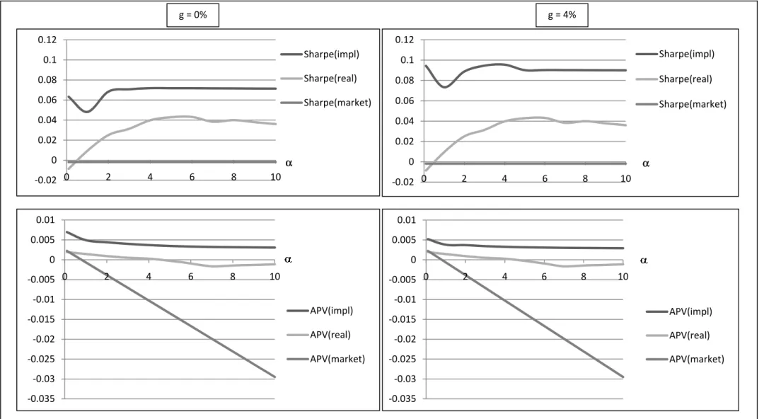
25 monthly returns. Optimal portfolios are computed for different growth rates g of expected annual dividend payments of 0 %, 1%, 2 %, 3 %, and 4 %. Risk aversion parameters are varied from 0.1 to 10. Moreover, short-sales restrictions are employed, as it is well-known that this generally leads to better results in the presence of estimation problems. For each different setting regarding and g and each of the two estimation procedures, an out-of-sample series of 110 rates of return of monthly optimized portfolios is obtained. For these actual portfolio return time series, we compute AP-values as defined above. Moreover, we calculate corresponding Sharpe ratios as a most common measure of comparison among different portfolio optimization techniques. Results are presented in Fig. 1 for annual growth rates of expected cash flows of g = 0 % and g = 4 % with “impl” and “real” denoting findings based on (13) and (15), respectively. Apparently, our empirical outcomes are in line with both our theoretical considerations and the results of our simulation: Portfolio optimization based on (13) leads to consistently better outcomes than portfolio selection based on (15). Moreover, portfolio selection according to (13) is unambiguously superior to simply holding the “market portfolio” or riskless lending (which would exhibit a Sharpe ratio and an AP-value of just 0). The market portfolio in our case is identical to the (time-varying) portfolio of stocks under consideration (results denoted by “market”). The same outcomes hold true for other annual growth rates between 0 % and 4 %. In fact, the only difference caused by variations of g is that the absolute level of the Sharpe ratio of the portfolio optimization based on (13) is affected, while the curvature remains almost completely the same. AP-values, in addition, are almost completely unaltered. This is quite remarkable, as the estimator according to (13) reacts sensitively to changes in g in a similar manner as the simple implied rate of return (for the latter problem see, e.g., Berg and Kaserer, 2008). However, the precise determination of g does not seem to be of major importance for the performance of the estimator according to (13) in actual portfolio selection problems.
26 As is well-known, there is a lack of powerful significance tests for differences in performance of alternative estimation methods. This is particularly true for the Jobson and Korkie (1981) test for significant differences in resulting Sharpe ratios (the same holds true for the correction of the Jobson and Korkie test presented in Memmel, 2003). In fact, although the differences reported in Fig. 1 for the resulting Sharpe ratios look economically significant, we cannot confirm statistically significant differences according to the Jobson and Korkie test. However, the purpose of Fig. 1 was simply to examine whether the finding for our bootstrap simulation does not contradict reality in an obvious way. Taking the results of this section and the preceding one together, we are convinced that the superiority of the estimation approach (13) in comparison to (15) can be concluded.
>>> Insert Fig. 1 about here <<<
Due to all these findings, it thus seems reasonable to employ (13) instead of (15) as the relevant estimation procedure in order to determine expected rates of return. Based on (15) for
= 36 for our real capital market data, one would get on average a monthly rate of return of 0.7762 % with a return standard deviation of this estimator of 1.5874 %. However, estimates for monthly expected future returns based on (13) are much lower even for an assumed annual growth rate of g = 4 %, as Table 5 reveals. At the same time, the standard deviation of this return estimator is indeed somewhat smaller than that of the standard estimator according to (15). In fact, estimates based on (13) are often negative and in general even smaller than when simply referring to the current implied rate of return as an expectation value estimator. Nevertheless, these estimators according to (13) do a good job in portfolio selection problems and are theoretically founded. In this sense, such estimators may prove superior. However, even if one should refer to these estimates, it remains an open issue whether such an estimator would be able to approximate market risk premia, because these reflect the assessment of the
27 whole capital market. The better an estimation procedure works in portfolio selection problems, the less representative corresponding estimates will be for the capital market as a whole. So, even if we started this paper with a reflection on the equity premium puzzle and although estimators according to (13) are quite low for our real capital market data and thus may contribute to a resolution of the equity premium puzzle, they may not be representative for capital market participants as a whole. Nevertheless, this problem holds true for each approach that aims at estimating future expected rates of return. In fact, for estimating market risk premia it seems that expectations are necessary that lead to the holding of the market portfolio. We therefore have to distinguish between these two goals of estimation procedures for expected rates of return: support of portfolio optimization and quantification of market risk premia. Both goals seem to be mutually exclusive. In this sense, our empirical findings may be understood as another reason why implied rates of return are not suited for market risk premia estimation even when based on equation (13).
>>> Insert Table 5 <<<
6 Conclusion
Implied rates of return are not suited for estimates of future one-period returns. The reason simply is the discrepancy between discount rates and expected returns. We derive analytically the relationship between implied rates of return and expected future returns and show that implied rates of return are on average a downward biased estimator for future one-period returns unless implied rates of return are constant over time. Moreover, we present an alternative estimation procedure based on the historical time series of implied rates of return and show theoretically its superiority to an estimator that is based on historical return realizations. Our theoretical findings are supported by a bootstrap approach and an empirical analysis. Rather interestingly, even for this newly introduced approach, resulting estimators of
28 expected rates of return seem to be smaller than in the case of estimates based on historical return realizations. In this sense, this new estimation procedure may also contribute to the resolution of the equity premium puzzle, although it does not lead to systematically downward biased estimates. However, it remains open to question whether this new estimation procedure (or any other alternative one) is able to approximate aggregate capital market expectations.
In this paper, we restricted ourselves to quite simple applications of the newly suggested optimization procedure. Certainly, it is possible to combine this approach with other methods, e.g. Bayesian estimation techniques, to improve portfolio selection techniques even more.
29 References
Barberis, N., Ming H., Tano S., 2001. Prospect Theory and Asset Prices. Quarterly Journal of Economics 116, 1-53.
Benartzi, S., Thaler, R. H., 1995. Myopic Loss Aversion and the Equity Premium Puzzle. Quarterly Journal of Economics 110, 73-92.
Berg, T., Kaserer, C., 2008. Estimating Equity Premia from CDS Spreads. SSRN Working Paper 2008.
Breuer, W., Fuchs, D., Mark, K., 2010. Estimating Cost of Capital in Firm Valuations with Arithmetic or Geometric Mean – or Better Use the Cooper Estimator?. SSRN Working Paper.
Butler, J. S., Schachter, B., 1989. The Investment Decision: Estimation Risk and Risk Adjusted Discount Rates. Financial Management 18, 13-22.
Capstaff, J., Paudyal, K., Rees, W., 2001. A Comparative Analysis of Earnings Forecasts in Europe. Journal of Business Finance and Accounting 28, 531-562.
Claus, J., Thomas, J., 2001. Equity Premia as Low as Three Percent? Evidence from Analyst’s Earnings Forecasts for Domestic and International Stock Markets. Journal of Finance 56, 1629-1666.
Constantinides, G., Donaldson, J., Mehra, R., 2002. Junior Can’t Borrow: A New Perspective on the Equity Premium Puzzle. Journal of Political Economy 98, 519-543.
Cooper, I., 1996. Arithmetic versus Geometric Mean Estimators: Setting Discount Rates for Capital Budgeting. European Financial Management 2, 157-167.
DeMiguel, V., Garlappi, L., Uppal, R., 2009. Optimal Versus Naive Diversification: How Inefficient is the 1/N Portfolio Strategy?. Review of Financial Studies 22, 1915-1953. DeLong, J. B., Magin, K., 2009. The U.S. Equity Return Premium: Past, Present, and Future.
Journal of Economic Perspectives 23, 193-208.
Easterwood, J. C., Nutt, S. R., 1999. Inefficiency in Analysts’ Earnings Forecasts: Systematic Misreaction or Systematic Optimism?. Journal of Finance 54, 1777-1797.
30 Fama, E. F., French, K. R., 1988. Dividend Yields and Expected Stock Returns. Journal of
Financial Economics 22, 3-25.
Fama, E. F., French, K. R., 2002. The Equity Premium. Journal of Finance 57, 637-659. Gebhardt, W. R., Lee, C. M. C., Swaminathan, B., 2001. Toward an Implied Cost of Capital.
Journal of Accounting Research 39, 135-176.
Graham, J. R., Campbell, H., 2007. The Equity Risk Premium in January 2007: Evidence from the Global CFO Outlook Survey. SSRN Working Paper.
Jobson, J. D., Korkie, B. M., 1981. Performance Hypothesis Testing with Sharpe and Treynor Measures. Journal of Finance 36, 889–908.
Johansen, S., 1991. Cointegration and Hypothesis Testing of Cointegration Vectors in Gaussian Vector Autoregressive Models. Econometrica 59, 1551–1580.
Kan, R., Zhou, G., 2007. Optimal Portfolio Choice with Parameter Uncertainty. Journal of Financial and Quantitative Analysis 42, 621-656.
Mankiw, N. G., Zeldes, S., 1991. The Consumption of Stockholders and Nonstockholders. Journal of Financial Economics 29, 97-112.
McGrattan, E. R., Prescott, E. C., 2003. Average Debt and Equity Returns: Puzzling?. Research Department Staff Report 313, Federal Reserve Bank of Minneapolis.
Mehra, R., Prescott, E. C., 1985. The Equity Premium: A Puzzle. Journal of Monetary Economics 15, 145-162.
Memmel, C., 2003. Performance Hypothesis Testing with the Sharpe Ratio. Finance Letters 1, 21–23.
Stickel, S. E., 1990. Predicting Individual Analyst Earnings Forecasts. Journal of Accounting Research 28, 409-417.
Welch, I., 2000. Views of Financial Economists on the Equity Premium and on Professional Controversies. Journal of Business 73, 501-537.
31 Appendix 1
Proof of Proposition 1 (ii):
According to (2), we have the following identity:
(impl) t 1 t 2 t 1 t 1 E (d ) r g . V (A1)
This in turn implies
t 1 t (impl) t t 1 t 1 t 2 (impl) t t 1 t 1 t 2 t t 1 V 1 E E and r g E (d ) 1 1 . E (r g) E (d ) E V ⎛ ⎞ ⎛ ⎞ ⎜ ⎟ ⎜ ⎟ ⎝ ⎠ ⎝ ⎠ ⎛ ⎞ ⎜ ⎟ ⎝ ⎠ (A2) Using (6) leads to t 1 t t (impl) t 1 t 1 t 2
(impl) (impl) (impl)
t t 1 t t 1 t t 1 t 2 (impl) t t t 1 V 1 g (1 g) E 1 E 1 r g E (d ) E (r ) r (1 r ) (1 r ) 1 E (d ) E r g V ⎛ ⎞ ⎛ ⎞ ⎜ ⎟ ⎜ ⎟ ⎝ ⎠ ⎝ ⎠ ⎛ ⎞ ⎜ ⎟ ⎝ ⎠ (A3)
and consequently (since from (2) we have (impl) t r / g 1) (impl) t 1 t 2 t 1 t t 1 t t t t 1 t 1 t 2 E (d ) V E (r ) r E E 1 0. g V E (d ) ⎛ ⎞ ⎛ ⎞ ⎜ ⎟ ⎜ ⎟ ⎝ ⎠ ⎝ ⎠ (A4)
The latter inequality immediately follows from Jensen’s inequality which implies
t 1 t t 1 t 2 t 1 t 2 t t 1 V 1 E . E (d ) E (d ) E V ⎛ ⎞ ⎜ ⎟ ⎛ ⎞ ⎝ ⎠ ⎜ ⎟ ⎝ ⎠ (A5)
Proof of Proposition 1 (iii): (6) immediately gives
(impl) (impl) (impl)
t t 1 t t t (impl) t t 1 1 g E (r ) r (r g) E 1 (1 r ). r g ⎛ ⎛ ⎞ ⎞ ⎜ ⎜ ⎟ ⎟ ⎜ ⎝ ⎠ ⎟ ⎝ ⎠ (A6)
32 Thus, it is sufficient to show the inequality
t (impl,B) t (impl,A) t 1 t 1 1 1 E E . r g r g ⎛ ⎞ ⎛ ⎞ ⎜ ⎟ ⎜ ⎟ ⎝ ⎠ ⎝ ⎠ (A7)
According to Jensen’s inequality, each realization (impl,A) t 1
r leads to
(impl,A)
t (impl,B) t 1 (impl,B) (impl,A) (impl,A) (impl,A) (impl,A)
t 1 t t 1 t 1 t 1 t t 1 t 1 1 1 1 1 E r r g E (r | r ) g r E ( | r ) g r g ⎛ ⎞ ⎜ ⎟ ⎜ ⎟ ⎝ ⎠ (A8)
which in turn implies the postulated result by taking expectations over all (impl,A) t 1
r
in (A8).
Appendix 2
Proof of Proposition 2:
Under consideration of (M) (A)
t t 1 t t 1
E (d ) / E (d ) 1, equation (11) immediately leads to the
inequality (impl,M) (impl,A)
t t
r r . The bias amounts to
(M)
(impl,M) (impl,A) (impl,A) t t 1
t t t (A) t t 1 E (d ) r r (r g) 1 E (d ) ⎛ ⎞ ⎜ ⎟ ⎝ ⎠ (A9) and thus (M)
(impl,M) (impl,A) (impl,A) t t 1
t t t (A) t t 1 E (d ) r r (r ) 1 1 0. g g E (d ) ⎛ ⎞ ⎛ ⎞ ⎜ ⎟ ⎜ ⎟ ⎝ ⎠ ⎝ ⎠ (A10) Appendix 3:
We show that the statements of Proposition 1 apply for unconditional expectations if we assume implied rates of return to be i.i.d.
Proof of Proposition 1 (i) for unconditional expectations: According to (6) we have (impl) t t 1 t t (impl) t 1 1 g E (r ) (r g) E 1 1. r g ⎛ ⎛ ⎞ ⎞ ⎜ ⎜ ⎟ ⎟ ⎜ ⎝ ⎠ ⎟ ⎝ ⎠ (A11)
33 Taking unconditional expectations on both sides of (A11) and considering rt(impl) and the
expectation value E ((1 g) / (rt t 1(impl) g)) to be independent leads to
(impl) t 1 t (impl) t 1 (impl) (impl) t (impl) t t 1 1 g E(r ) (E(r ) g) E 1 1 r g 1 g (E(r ) g) 1 1 E(r ). E(r ) g ⎛ ⎛ ⎞ ⎞ ⎜ ⎜ ⎟ ⎟ ⎜ ⎝ ⎠ ⎟ ⎝ ⎠ ⎛ ⎞ ⎜ ⎟ ⎝ ⎠ (A12)
The latter equality results from the fact that implied rates of return are assumed to be
identically distributed over time. The inequality in (A12) only holds if the variance of (impl) t
r
is
positive. Otherwise, we immediately get (impl)
t 1 t
E(r ) r .
Proof of Proposition 1 (ii) for unconditional expectations:
(A1) under consideration of the i.i.d. property of the implied rates of return leads to
t 1 (impl) t 1 t 1 t 2 (impl) (impl) t 1 t 2 t t 1 t 1 V 1 E E , r g E (d ) E (d ) E(r ) g E(r g) E . V ⎛ ⎞ ⎛ ⎞ ⎜ ⎟ ⎜ ⎟ ⎝ ⎠ ⎝ ⎠ ⎛ ⎞ ⎜ ⎟ ⎝ ⎠ (A13)
Using these identities in (A12) immediately implies
(impl) t 1 t 2 t 1 (impl) t 1 t t t 1 t 1 t 2 E (d ) V E(r r ) E (1 g) E 1 (1 E(r )). V E (d ) ⎛ ⎞ ⎛ ⎞ ⎛ ⎞ ⎜ ⎟ ⎜ ⎟ ⎜ ⎜ ⎟ ⎟ ⎝ ⎠ ⎝ ⎝ ⎠ ⎠ (A14)
The rest of the proof is analogous to (A4) and (A5) if we replace conditional expectations by unconditional expectations.
Proof of Proposition 1 (iii) for unconditional expectations: Under consideration of
(impl) (impl) (impl)
t 1 t t (impl) t
t 1
1 g
E(r r ) (E(r ) g) E 1 (1 E(r ))
r g ⎛ ⎛ ⎞ ⎞ ⎜ ⎜ ⎟ ⎟ ⎜ ⎝ ⎠ ⎟ ⎝ ⎠ (A15)
34
and (impl,A) (impl,B)
t t
E(r ) E(r ) the proof proceeds analogously to the proof of part (iii) of Proposition 1.
Appendix 4:
Proof of the Lemma:
With : h(x, y) f (x) we have h(x, y) f (x) . If we consider an arbitrary realization x of
x, we immediately get the following relationship
E( | x x) E(h(x, y) | x x) f (x) 0. (A16)
Thus, h(x, y) is a mean preserving spread of f (x) .
Appendix 5:
Proof of Proposition 3 (ii):
From (5), we know that (impl) (impl)
t 1 t t 1 t 1 t 1 t 2
r : h(r , r , d , E (d ))
depends on three random
variables dt 1, E (d )t 1 t 2 and (impl) t 1 r , whereby (impl) t 1 r is independent of E (d )t 1 t 2 . If we
additionally define f according to (impl) (impl) (impl) (impl)
t t 1 t 1
f (r , r ) : (r g) (1 g) / (r g) 1 1, equation (6) implies:
(impl) (impl) (impl) (impl) (impl) (impl)
t t t 1 t 1 t 1 t 2 t 1 t (impl) t t 1 t 1 1 g E (h(r , r , d , E (d ) r ) (r g) 1 1 f (r , r ). r g ⎛ ⎞ ⎜ ⎟ ⎝ ⎠ (A17)
According to the Lemma, rt 1 is a conditional mean preserving spread of (impl) (impl)
t t 1
f (r , r ). On this basis, we define (impl)
1(r )
as that random variable which implies
(impl) (impl) (impl) (impl) (impl) (impl)
1 1 1 t 1 1 1
r f (r , r ) (r ) and E ( (r ) | r ) 0 for all r .
(A18)
With the abbreviation (impl)
1: 1(r )
, this result can be generalized to an “unconditional” statement, since obviously
(impl) (impl) (impl) (impl) (impl) (impl)
1 1 1 1 1 1
r f (r , r ) and E( | r , r ) 0 for all (r , r ).
35 Proof of Proposition 3 (iii):
With function f from above we have (impl) t 1 (impl) (impl)
t , t 1
µ (1 / )
∑
f (r , r ). Since for each the return r 1 is a mean preserving spread of (impl) (impl)1
f (r , r ), we are able to define the random variable : (1 / )
∑
t 1t 1 which immediately leads to(real) (impl) (impl) (impl) (impl) (impl) (impl)
t, t, t, t t t t
µ µ and E( | µ ) E( | r , ..., r ) 0 for all (r , ..., r ). (A20)
Thus, (real) t,
µ is a mean preserving spread of (impl) t,
µ .
Appendix 6:
Proof of the Corollary:
In the following, we identify riskless lending or borrowing with security i = 0 and define
(impl)* i
x (i = 0, 1, …, N) as the optimal fraction of wealth invested in security i if the investor
bases his or her estimation of expected returns on (13). In addition, (real)* i
x (i = 0, 1, …, N)
stands for the corresponding fraction if the decision relies on the application of (15).
Furthermore, we define (impl) i,t 1
r
as the estimated uncertain return of the next period on the basis
of (13) and (real) i,t 1
r
as the corresponding return estimated according to (15). For all portfolios P
= (x0, x1, …, xN), the portfolio return estimations
N
(impl) (impl) (c) (impl) (c)
P,t 1 P,t, P,t 1 0 f i i,t, P,t 1
i 1 N
(real) (real) (c) (real) (c)
P,t 1 P,t, P,t 1 0 f i i,t, P,t 1 i 1 r r x r x µ r and r r x r x µ r
∑
∑
(A21)and the statement of Proposition 3 immediately imply (real) P,t 1
r
to be a mean preserving spread of
(impl) P,t 1
r
. Thus, for all portfolios P and an arbitrary (strictly increasing and concave) utility
function U we obtain the inequality
(impl) (real)
P,t 1 P,t 1
36 If we denote (impl)* (impl)* (impl)* (impl)*
0 1 N
P (x , x , ..., x ) and (real)* (real)* (real)* (real)*
0 1 N
P (x , x , ..., x ) we
finally get the postulated statement
(impl)* ( real)* ( real)*
(impl) (impl) (real)
P ,t 1 P ,t 1 P ,t 1
E U(r⎡⎣ )⎤⎦ E U(r⎡⎣ )⎦⎤ E U(r⎡⎣ ) .⎤⎦ (A23)
The first inequality is a result of the optimality of P(impl)* in the “estimation case” (13) and the