Individual Financial Analysts’ Contribution
In Earnings Per Share Forecasting
Marc A. Giullian (Email: mgiullian@montana.edu), Montana State University-Bozeman Abstract
Financial analysts are among the most influential group of users of financial accounting information. The majority of existing accounting research concerning financial analysts focuses on aggregated analysts' earnings forecasts rather than individual analysts' forecasts. Studies in accounting have documented the superiority of aggregated analysts' earnings forecasts relative to computer models. This is in contrast to the robust result from years of psychology/judgment & decision making (JDM) research that human predictions are inferior to computer model predictions. Humans can make a significant contribution to accurate forecasting in spite of cognitive limitations. Some skills people bring to bear are cue identification, rapid adaptability to environmental changes and the evaluation of qualitative factors. Computer models offer consistency and significant computational power. This research documents the incremental predictive ability of both individual financial analysts and computer models in forecasting earnings per share. It also provides evidence that both individual financial analysts' and computer models' incremental predictive ability varies between industries.
1.0 Introduction
ver the last two decades, interest in forecasts of corporate earnings has grown significantly. Forecasting earnings is one of the vital services performed by financial analysts (Knutson, 1993). Today, thousands of analysts earn their livelihood from monitoring, studying and forecasting earnings in addition to other activities (e.g. selecting stocks).1 An indication of this increasing interest is the substantial growth in commercially available earnings forecasting services
Financial analysts significantly influence the investment decisions of investors. For example, a study sponsored by the Financial Executives Research Foundation (FERF) indicates that "The advisor-dependent approach to decision making is typical of perhaps 50 percent of all individual investors..." (SRI International, 1987, p.26). Similarly, Schipper (1991) argues that
Given their importance as intermediaries who receive and process financial information for investors, it makes sense to view analysts--sophisticated users--as representative of the group to whom financial reporting is and should be addressed (p. 105).
Studying financial analysts is important because they arguably constitute the most significant group of financial accounting information users. While financial analysts perform a variety of tasks as users of financial accounting information, the predictive judgment of forecasting earnings per share is the focus of this paper.
2.0 Human Information Processing and Predictive Judgment
A large body of psychology/judgment & decision making literature documents humans’ inferiority to computer models in predictive judgment (Meehl, 1954; Sawyer, 1966; Ebert & Kruse, 1978; Dawes, 1979; Kleinmuntz, 1990). Hypothesized causes this inferiority are numerous. Probably the most oft-cited cause is limited ____________________
Readers with comments or questions are encouraged to contact the author via emal.
information processing capacity (Simon, 1955). When decisions must be made in an environment characterized by the need for fast, accurate computations, people do not perform well. Even when sufficient time is available to perform optimally, people may still fail to do so. This could be because of unwillingness to expend the required mental effort (cognitive costs) or because of computational errors made during the process (Payne, Bettman & Johnson, 1993). Other causes of poor human performance suggested in the literature are fatigue, emotion, perceptual biases, overconfidence, organizational politics and reputation enhancement (Fischhoff, Slovic & Lichtenstein, 1977).
Notwithstanding these limitations, humans do possess abilities that are helpful in making accurate predictions. Cue identification is one example. The ability to recognize variables useful in predicting future events most likely results from humans' ability to learn and understand causal relationships. Humans are clearly superior to models at learning and building causal connections that relate occurrences of one event to the likelihood of occurrence of another. This ability is especially useful in cases where rare but highly diagnostic cues (broken-leg cues) are present (Meehl, 1954). For example, if one was building a model to predict outcomes for individuals in a women's Olympic figure skating championship, variables such as past performance in the technical program and long program would probably be included. However, if one of the contestants was assaulted and intentionally injured a month before the competition, this would probably prevent that contestant from winning. This type of cue would be very easy for a person to utilize in their predictive judgment.
Humans also possess the ability to rapidly and effectively adapt to changes in decision environments. Because people can recognize changes in causal relationships, they can adapt their knowledge of a particular predictive domain to incorporate environmental changes. Obviously, models do not have this ability. Changes cannot be incorporated until the model builders make the needed adjustments. Thus, if predictions are needed in a domain characterized by a rapidly changing environment, the adaptability of humans will help them predict more accurately than relatively inflexible, computer models.
Finally, humans have the ability to evaluate qualitative factors.2 Subjective variables are of little use to statistical models because they are typically not stated in quantitative terms. Only when such variables are translated by humans can they be utilized by models. In summary, humans can contribute important skills to improving predictions, namely cue identification, rapid adaptability to dynamic predictive environments and subjective variable assessment.
3.0 Computer Model Prediction
As mentioned earlier, computer model predictions have been shown to be generally more accurate than human predictions. This is because of the strengths inherent in models when making predictions. For example, computer models have huge computational capacity, are immune to fatigue, emotion and perceptual biases. However, computer models are not a panacea for universally improving predictions. Models also have weaknesses. For example, models cannot perform any of the judgmental tasks required in building models. Such tasks could include determining the appropriate independent variables, determining the appropriate functional form, specifying the appropriate autocorrelation structure, etc. Models are also not able to utilize rare but diagnostic cues when they are available. Furthermore, models cannot easily judge subjective, but nevertheless, predictive variables. Finally, models are not well-suited to adapt to changing environments. This could be a significant challenge in predicting earnings. Thomas (1993) discusses evidence suggesting that the process generating earnings has slowly changed over the last 30 years. There is also evidence suggesting that the earnings generation process differs from firm to firm and that these processes are nonstationary rather than stationary (Ziebart, 1987). Assuming the earnings generation process is dynamic, the ideas discussed earlier predict that human forecasts will outperform computer model forecasts.
4.0 The Adaptive Decision Maker
Payne, Bettman & Johnson (1993) have developed a characterization of human decision makers known as the adaptive decision maker. The fundamental idea behind their work is that human decision strategy choice is
based on trade offs between the amount of perceived effort required to use a certain strategy and the perceived level of accuracy of that strategy. People will prefer a strategy wherein they perceive that accuracy can be increased with a slight increase in perceived effort. One strategy that offers this type of trade off is the use of broken-leg cues. Johnson (1988) provides evidence that humans rely heavily upon this type of cue in making predictive judgments. His study was in the context of experienced physicians ranking applicants for prestigious medical residencies and internships. The physicians reviewed applicants’ folders and then ranked the applicants in order of their likelihood for success in the desired residency or internship. Johnson found that the experienced physicians emphasized information unique to the applicant (broken-leg cues) and ignored information common to all applicants.
The data typically ignored by people are the data typically utilized by models. While people tend to examine different data for each case being judged (depending on the case's unique features), models examine the same variables for every case (Hoch & Schkade, 1996). A computer model would not be likely to contain case specific variables because of their infrequency of occurrence, but a person could effectively utilize these kinds of cues in predicting an outcome. However, highly predictive, case-specific data are usually not available for all cases. Thus, people cannot fully utilize their comparative strength in making their judgments. As a result, human performance, on average, is generally inferior to models since models use data that are available for every case. In essence, people tend to rely upon their inherent comparative strength of utilizing unique data and tend to ignore common data when making predictive judgments. The rationale for this behavior is people's perception that their desired accuracy can be achieved with much less effort using unique instead of common data. This is consistent with the idea that people make trade-offs between effort and accuracy when faced with tasks requiring mental effort (Payne, Bettman & Johnson, 1993).
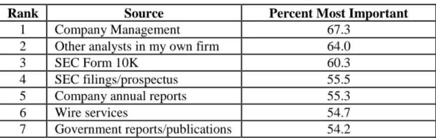
Whether or not they are explicitly aware of these tendencies, financial analysts exhibit this same type of behavior in making judgments about a firm’s earnings. As shown in Table 1 below, financial analysts list firm management as the most important information source (SRI International, 1987, reproduction of Table 4.6). One explanation for this preference is that analysts seek to utilize their ability to integrate "broken-leg" cues into their judgments. Assuming "broken-leg" cues are most likely to be qualitative, it seems sensible for analysts to earnestly seek for qualitative information from management. Similarly, analysts have a strong preference for timely information. This preference may result from the analysts' desire to capitalize on their ability to quickly adapt to new information. The sooner new data are received, the sooner they can be integrated into mental models and forecasts. Because more timely forecasts have been shown to be more accurate (O'Brien, 1988), analysts are likely to have a strong preference for timely information. Thus, analyst behavior seems consistent with the idea that people tend to rely upon their strengths when making judgments such as earnings forecasts.
TABLE 1: Investor Information Needs and the Annual Report (SRI International) Importance of Information Sources
Rank Source Percent Most Important
1 Company Management 67.3
2 Other analysts in my own firm 64.0
3 SEC Form 10K 60.3
4 SEC filings/prospectus 55.5
5 Company annual reports 55.3
6 Wire services 54.7
7 Government reports/publications 54.2
5.0 Research Method
The data needed to investigate the incremental predictive ability of financial analysts in forecasting earnings per share includes individual analysts’ quarterly earnings per share forecasts, firms’ actual quarterly earnings per share and other economic data. The selection of firms used in this study was constrained by two factors. The first was the number of analysts forecasting EPS for a given firm. Firms with less than five analysts
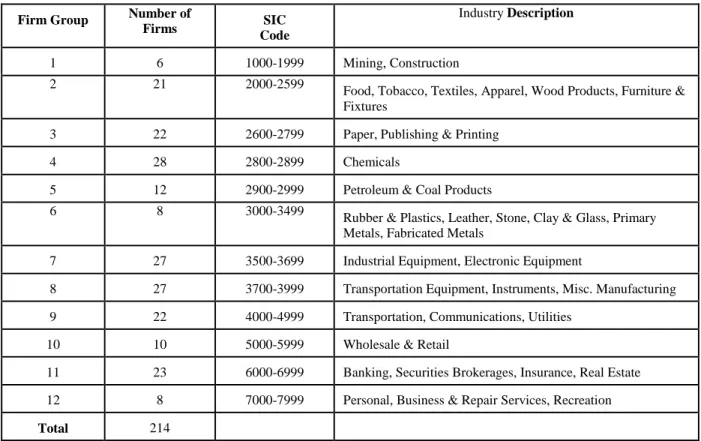
providing forecasts were eliminated. Of the 595 firms that were included in both the I/B/E/S and Compustat databases, 256 had five or more analysts with a 12 out of 16 forecasts between the first quarter of 1990 and the last quarter of 1993. Another constraint was data availability for the generation of computer model forecasts. Forty firms had insufficient historical data resulting in a final sample of 214. Firms were grouped according to SIC codes to facilitate industry analysis. Twelve groups resulted from this grouping and the details are shown in Table 2.
TABLE 2: Details of Firm Group Categories
Firm Group Number of
Firms SIC
Code
Industry Description
1 6 1000-1999 Mining, Construction
2 21 2000-2599
Food, Tobacco, Textiles, Apparel, Wood Products, Furniture & Fixtures
3 22 2600-2799 Paper, Publishing & Printing
4 28 2800-2899 Chemicals
5 12 2900-2999 Petroleum & Coal Products
6 8 3000-3499
Rubber & Plastics, Leather, Stone, Clay & Glass, Primary Metals, Fabricated Metals
7 27 3500-3699 Industrial Equipment, Electronic Equipment
8 27 3700-3999 Transportation Equipment, Instruments, Misc. Manufacturing 9 22 4000-4999 Transportation, Communications, Utilities
10 10 5000-5999 Wholesale & Retail
11 23 6000-6999 Banking, Securities Brokerages, Insurance, Real Estate 12 8 7000-7999 Personal, Business & Repair Services, Recreation
Total 214
Quarterly data from the years 1990-1993 were used for all analyses. The purpose of examining four years of data was to reduce the size of the data set to a manageable level. Limiting firms rather than time periods was also considered as a constraint. However, limiting firms would have reduced the total number of analysts included in the study since analysts tend to follow firms across time. Since the focus of this study was individual analysts' forecasts, it was more important to maximize the number of analysts rather than the number of time periods included in the study. Balancing the size of the data set with the objective of maximizing the number of analysts was most effectively accomplished by imposing the time period constraint noted above.
The final data set consisted of the twelve quarters starting with the second quarter of 1990 and ending with the first quarter of 1993. All 16 quarters between 1990 and 1993 could not be used because of missing data points for many individual analysts. The quarters not included in the analysis (1st quarter of 1990 & 2nd, 3rd & 4th quarter of 1993) were eliminated because they had the highest occurrence of missing data points among the individual analysts. The rates of missing data for the eliminated quarters were 14%, 19%, 16% and 19%, respectively.
Some analysts had missing data in quarters other than those that were eliminated. When this was the case, these missing data points were filled in. The method used sought to shift the fewest number of forecasts possible to fill in the missing forecast. If the missing forecast was in the first two years of the test period (1990-1991), any
preceding forecasts were shifted forward to fill in the gap. If the missing forecast was in the last two years of the test period (1992-1993), any subsequent forecasts were shifted backward to fill in the gap.
The main benefit to this procedure was the facilitation of the analysis. The sample size would have been significantly reduced had this not been done because any series of analyst's forecasts with a missing forecast would be ignored by the software used for the analysis. The cost of this procedure is that no inferences can be drawn about specific periods. The benefit outweighed the cost because the focus of this study is on analysts, not time periods and making these data substitutions allowed for the most analysts to be included in the analysis.
6.0 Data Sources
Individual analysts' and summary analysts' forecasts of quarterly EPS were gathered from the I/B/E/S database for the years 1990-1993.3 Computer model forecasts were generated using historical data. The capital markets literature offers a myriad of models for forecasting quarterly EPS. ARIMA-type models are identified in accounting literature as reliable for forecasting quarterly earnings (Brown et al, 1987a). The ARIMA model developed by Brown and Rozeff (1979) is one such model. Research has shown this model to be the most accurate of those commonly used in the accounting literature (Bathke & Lorek, 1984). In addition to this model, hybrid models that utilized both times series data and macroeconomic data were estimated and used to generate forecasts. This was done by modifying the Brown-Rozeff model. Thus, for each firm, five model forecasts were estimated: a time series model and four hybrid models. Quarterly data from 1980 to 1989 were used to estimate the models. Computer model forecasts were generated for each quarter of the years 1990 to 1993. The forecasts from each model for a given firm were compared to the actual values for the same firm to determine the most accurate model forecast.4 Only the most accurate model forecast was used in the analysis. Actual EPS (excluding extraordinary items) data were taken from Compustat. Although I/B/E/S provides actual EPS values, researchers have found Compustat to be a more reliable source of quarterly EPS data (Philbrick & Ricks, 1991).
7.0 Analysis
The incremental predictive ability of analysts and models was examined using regression analysis. The first test performed was to determine the existence of incremental predictive ability for both individual analysts and models. The first step in performing this test was to run a full effects regression model. The regression equation used for this step was as follows:
EPSjt = bo+b1MFjt+b2AF1jt+b3AF2jt+b4AF3jt+b5AF4jt+b6AF5jt+ejt, (1)
Where
EPSjt = Quarterly EPS for firm j, period t,
AFijt = Analyst's Forecast for analyst i, firm j, period t,
MFjt = Model Forecast for firm j, period t,
ejt = Error term for firm j, period t.
Two reduced model regressions were then run. First, the model forecast was removed from equation (1) leaving only the analysts' forecasts. Then all the analysts' forecasts were removed from equation (1), leaving only the model forecast. An F statistic was constructed using the sum of squared errors for each of the three regressions to test whether or not the increment in variance explained was significantly different from zero (Neter, Wasserman & Kutner, 1985, p. 290-291). The hypothesis regarding incremental predictive ability is that both model forecasts and the analysts' forecasts will add a significant amount of explanatory power. This is consistent with research in other domains wherein the idea of incremental predictive ability has been examined (Blattberg & Hoch, 1990). It is also consistent with research suggesting that people do not fully integrate time series properties of earnings into their forecasts (Hand & Maines, 1994).
An interesting finding from O'Brien (1990) is that some firms' earnings are easier to predict than others. This finding is extended by examining whether or not there is a differential incremental contribution made by analysts based on industry. For example, some industries may exhibit relatively stable earnings (e.g. public utilities) whereas others are likely to be volatile (e.g. biotechnology). Analysts may contribute relatively less to forecast accuracy in stable industries as opposed to volatile industries. Regression was used to examine the issue of differing incremental predictive ability between industries. The first step of this analysis was to regress the individual analysts' forecasts on the model forecast for a given firm and quarter. The purpose of this regression was to identify the portion of the model forecast that is not shared with the analysts' forecasts. The regression equation used is as follows:
MFjt = co + c1AFijt + eijt, (2)
Where
AFijt = Analyst's Forecast for analyst i, firm j, period t,
MFjt = Model Forecast for firm j, period t,
eijt = Error term for analyst i, firm j, period t.
This regression was run with each of the five individual analysts' forecasts. The residuals from these five regressions were then used as independent variables in another regression to test for differential incremental predictive ability between industries. In addition to the five sets of residuals from equation (2), eleven dummy variables were crossed with the five residual variables and added to this regression equation. The regression equation is as follows:
EPSjt = do + d1e1jt + d2e2jt + d3e3jt + d4e4jt + d5e5jt + d6(DUM1*e1jt) + ... + d60(DUM11*e5jt) + ujt, (3)
Where
EPSjt = Quarterly EPS for firm j, period t,
DUMi = Dummy variable for firm group i,
eijt = Residual term from equation (2) for analyst i, firm j, period t,
ujt = Error term for firm j, period t.
After this model was run, a reduced model was run. The reduced model is as follows:
EPSjt = do + d1e1jt + d2e2jt + d3e3jt + d4e4jt + d5e5jt + ujt (4)
The basis of this analysis was to compute an F statistic to determine if there was a significant amount of incremental explained variance between the full model and the reduced model.
8.0 Results
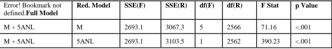
The results of the first analysis indicate that both individual analysts' forecasts and model forecasts exhibit incremental predictive ability. The results of this statistical test are reported in Table 3A. The results in which the reduced model includes only the model forecasts indicates that adding the five individual analysts' as independent variables significantly increases the amount of variance explained (F(5,2566)=71.16, p<.001). Likewise, when the reduced model includes only the individual analysts' forecasts, adding the model forecasts results in a significant increase in the amount of variance explained (F(1,2562)=390.23, p<.001). As hypothesized, both individual analysts' forecasts and model forecasts possess significant incremental predictive ability.
TABLE 3A: F Statistic Computations for Incremental Predictive Ability Analysis Using Data for All Individual Analysts Error! Bookmark not
defined.Full Model
Red. Model SSE(F) SSE(R) df(F) df(R) F Stat p Value
M + 5ANL M 2693.1 3067.3 5 2566 71.16 <.001
M + 5ANL 5ANL 2693.1 3103.5 1 2562 390.23 <.001
Another part of the incremental predictive ability analysis examined whether or not analysts and models exhibit differential incremental predictive ability between industries. This analysis also utilizes the strategy of estimating a full model and a reduced model and then examining the increment in explained variance. When the analysts' unique predictive contributions (residual from regression of individual analysts' forecasts on model forecasts) were used as independent variables (as well as being crossed with dummy variables for industry groups), there was a significant increment in explained variance. Similarly, when the models' unique predictive contributions (residual from regression of model forecasts on individual analysts' forecasts) were used as independent variables (as well as being crossed with dummy variables for industry groups), there was a significant increment in explained variance. These results are shown in Tables 4A and 4B.
TABLE 4A: Overall Test for Differential Incremental Predictive Ability Using Analysts' Unique Predictive Contribution Error! Bookmark not
defined.SSE(F)
SSE(R) df(F) df(R) F Stat p Value
3370.8 3805.3 55 2562 5.875 <.001
Full Model
EPSjt = do + d1e1jt + d2e2jt + d3e3jt + d4e4jt + d5e5jt + d6(DUM1*e1jt) + ... + d60(DUM11*e5jt) + ujt,
Reduced Model
EPSjt = do + d1e1jt + d2e2jt + d3e3jt + d4e4jt + d5e5jt + ujt
EPSjt = Quarterly EPS for firm j, period t,
DUMi = Dummy variable for firm group i,
eijt = Residual term with Ai as dep var. and M as indep var. for analyst i, firm j, period t,
ujt = Error term for firm j, period t.
TABLE 4B: Overall Test for Differential Incremental Predictive Ability Using Model's Unique Predictive Contribution
SSE(F) SSE(R) df(F) df(R) F Stat p Value
2854.6 3257.1 55 2562 6.428 <.001
EPSjt = do + d1e1jt + d2e2jt + d3e3jt + d4e4jt + d5e5jt + d6(DUM1*e1jt) + ... + d60(DUM11*e5jt) + ujt,
Reduced Model
EPSjt = do + d1e1jt + d2e2jt + d3e3jt + d4e4jt + d5e5jt + ujt
EPSjt = Quarterly EPS for firm j, period t,
DUMi = Dummy variable for firm group i,
eijt = Residual term with M as dependent var. and Ai as independent var. for analyst i, firm j, period t,
ujt = Error term for firm j, period t.
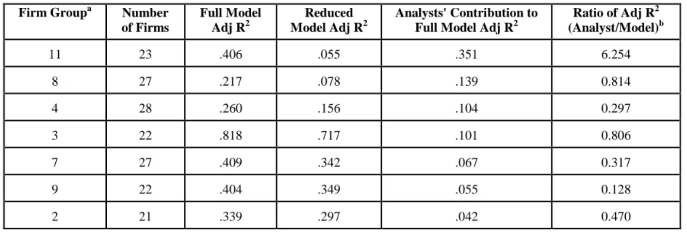
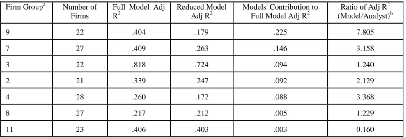
However, these overall results did not reveal which specific industries were more or less easily predicted. In order to disentangle this relationship, two additional analyses were done. First, full and reduced models (based on equation 1) were estimated for each of the 12 firm groups. The differences in adjusted R2 between the full and reduced models for each group were computed and are reported in Tables 5A and 5B. Results for the groups with fewer than 20 analysts are considered unreliable due to small sample size and are not reported. The second analysis used both sets of residuals (model regressed on analysts and vice versa) computed in equation 2. Both sets of residuals were then regressed on actual EPS for the firm groups with more than 20 firms. The adjusted R2 from these two regressions were used to form a ratio for each firm group. These ratios are reported in the sixth column of Tables 5A and 5B. The results of these analyses suggest some support for the hypothesized differences in incremental predictive ability. The rankings in Tables 5A and 5B are in decreasing order of incremental predictive ability. The analysts displayed the greatest incremental predictive ability in the Banking, Securities Brokerages, Insurance and Real Estate industry (group 11) while the models displayed the least incremental predictive ability for this industry. The industry in which models showed the greatest incremental predictive ability, Transportation, Communication and Utilities (group 9), was also the one in which the analysts showed the second least incremental predictive ability. The ratios shown in the last column of Tables 5A and 5B bolster this result.
TABLE 5B: Differential Incremental Predictive Ability Analysis For Analysts
Firm Groupa Number
of Firms Full Model Adj R2 Reduced Model Adj R2 Analysts' Contribution to Full Model Adj R2
Ratio of Adj R2 (Analyst/Model)b 11 23 .406 .055 .351 6.254 8 27 .217 .078 .139 0.814 4 28 .260 .156 .104 0.297 3 22 .818 .717 .101 0.806 7 27 .409 .342 .067 0.317 9 22 .404 .349 .055 0.128 2 21 .339 .297 .042 0.470 a
The industry descriptions of the firm groups included in this table are as follows: 11 - Banking, Securities Brokerages, Insurance, Real Estate,
8 - Transportation Equipment, Instruments, Misc. Manufacturing, 4 - Chemicals,
3 - Paper, Publishing & Printing
7 - Industrial Equipment, Electronic Equipment 9 - Transportation, Communications, Utilities
2 - Food, Tobacco, Textiles, Apparel, Wood Products, Furniture & Fixtures
b
The Adjusted R2 figures used to form the ratios in this column are from different regressions than the other columns in the table. The ratios are based on equation 6 which is repeated here for convenience:
EPSjt = do + d1e1jt + d2e2jt + d3e3jt + d4e4jt + d5e5jt + ujt
This regression was run with the analysts' unique predictive contribution (eitj from AFijt = c0 + c1MFjt + eijt) as the independent
variable and then with the model's unique predictive contribution (eitj from MFjt = c0 + c1AFijt + eijt) as the independent variable.
The Adjusted R2 from these two regressions were then used to form the ratios reported in this column. For this table, the Adjusted R2 from the regression with the analysts' unique predictive contribution as independent variable was the numerator of the ratio reported.
TABLE 5B: Differential Incremental Predictive Ability Analysis For Models Firm Groupa Number of
Firms
Full Model Adj R2
Reduced Model Adj R2
Models' Contribution to Full Model Adj R2
Ratio of Adj R2 (Model/Analyst)b 9 22 .404 .179 .225 7.805 7 27 .409 .263 .146 3.158 3 22 .818 .724 .094 1.240 2 21 .339 .247 .092 2.129 4 28 .260 .172 .088 3.368 8 27 .217 .212 .005 1.229 11 23 .406 .403 .003 0.160 a
The industry descriptions of the firm groups included in this table are as follows: 9 - Transportation, Communications, Utilities,
7 - Industrial Equipment, Electronic Equipment, 3 - Paper, Publishing & Printing,
2 - Food, Tobacco, Textiles, Apparel, Wood Products, Furniture & Fixtures, 4 - Chemicals,
8 - Transportation Equipment, Instruments, Misc. Manufacturing, 11 - Banking, Securities Brokerages, Insurance, Real Estate.
b
The Adjusted R2 figures used to form the ratios in this column are from different regressions than the other columns in the table. The ratios are based on equation 6 which is repeated here for convenience:
EPSjt = do + d1e1jt + d2e2jt + d3e3jt + d4e4jt + d5e5jt + ujt
This regression was run with the analysts' unique predictive contribution (eitj from AFijt = c0 + c1MFjt + eijt) as the independent
variable and then with the model's unique predictive contribution (eitj from MFjt = c0 + c1AFijt + eijt) as the independent variable.
The Adjusted R2 from these two regressions were then used to form the ratios reported in this column. For this table, the Adjusted R2 from the regression with the model's unique predictive contribution as independent variable was the numerator of the ratio reported.
9.0 Conclusion
The results from this analysis strongly support the conclusion that individual financial analysts exhibit predictive ability above that possessed by models and vice versa. Analysts and models also share a common portion of predictive ability. A simple Venn diagram illustrates this point. In Figure 1, the large circle represents the total variance to be explained in forecasting EPS. The smaller circle labeled A represents the analysts' forecasts. The smaller circle labeled M represents the model forecasts. The intersection of circles A and M that is inside the larger circle represents the portion of variance both analyst and model explain (area 2). The area of intersection between circle A and the larger circle that is not shared with circle M represents variance explained solely by the analysts'
forecasts (area 1). In this study, this increment in explained variance is equal to .088 (.354 {Full model adjusted R2 } - .266 {reduced model adjusted R2}). The intersection between circle M and the larger circle that is not shared with circle A represents variance explained solely by the model forecasts (area 3). The amount of the increment of explained variance in this case is .098 (.354 - .256). Thus, it seems that the unique elements of predictive ability possessed by the analysts and models are smaller than the portion that is common to both. There appears to be a modest but significant increase in the amount of explained variance as indicated by the analysis. This result is consistent with the idea that both analysts and model possess strengths in making forecasts that are somewhat complementary.
The differential incremental predictive ability results suggest that individual analysts and computer models contribute differentially in forecasting earnings for different industries. There is some support for the hypothesis that analysts contribute more to predictive ability when used for forecasting earnings in less stable industries than in more stable industries. Likewise, there is some support for the hypothesis that models contribute more to predictive ability when used for forecasting earnings in more stable industries than in less stable industries. The rankings of industries by incremental predictive ability results show somewhat of an inverse pattern. Those industries in which analysts tend to contribute more to predictive ability are those in which models tend to contribute less and vice versa. Other tests could be devised that would likely yield more focused results. For example, a finer distinction (based on SIC code) than that used in this study could be used along with a larger number of analysts' forecasts to ensure sufficiently large sample sizes. Such a test would give more focused results than this study about specific industries.
Recent events5 are likely to fundamentally change the environment in which financial analysts make their forecasts of firms’ earnings per share. Concerns about the incentives investment banking firms offer to financial analysts has been the catalyst behind a proposal to separate of investment research from related investment banking services. The SEC is currently weighing the proposal in effort to remove a motivational bias on the part of financial analysts to overstate firms’ earnings per share. In spite of these changes, the usefulness of analysts’ EPS forecasts will continue given the strong relationship between a firms’ earnings and its stock price. This new environment, whatever it ends up being, will hopefully provide an opportunity for continued study of financial analysts’ forecasts.
References
1. Bathke, A. W., Jr., and K. S. Lorek, (1984) The relationship between time-series models and the security market's expectation of quarterly earnings. The Accounting Review, 59, 49-68.
2. Blattberg, R. C., and S. J. Hoch. (1990). Database models and managerial intuition: 50% model and 50% manager. Management Science, 36, 887-899.
3. Brown, L. D., R. Hagerman, P. Griffin and M. Zmijewski (1987a). Security analyst superiority relative to univariate time-series models in forecasting quarterly earnings. Journal of Accounting and Economics, 9, 61-87.
4. Brown, L. D. and M. S. Rozeff (1978). The superiority of analyst forecasts as measures of expectations.
Journal of Finance, 33, 1-16.
5. Dawes, R. M. (1979). The robust beauty of improper linear models in decision making. American
Psychologist, 34, 571-582.
6. Ebert, R. and T. Kruse (1978). Bootstrapping the security analyst. Journal of Applied Psychology, 63, 110-119.
7. Einhorn, H. J. (1972). Expert measurement and mechanical combination. Organizational Behavior and
Human Performance, 7, 86-106.
8. Fischhoff, B., P. Slovic and S. Lichtenstein (1977). Knowing with certainty: the appropriateness of extreme confidence. Journal of Experimental Psychology: Human Perception and Performance, 3, 522-564.
9. Hand, J. R. M., and L. Maines (1994) The ability of individuals to forecast quarterly earnings per share series with varying time-series complexities. Working paper, University of North Carolina (first author) and Duke University (second author).
10. Hoch, S. J. and D. A. Schkade (1996) A psychological approach to decision support systems, Management
Science, 42, 51-64.
11. Johnson, E. J. (1988). Expertise and decision under uncertainty: performance and process, in The Nature of
Expertise, M. T. H. Chi, R. Glaser and M. J. Farr (Eds), Erlbaum, Hillsdale, NJ.
12. Kleinmuntz, B. (1990). Why we still use our heads instead of formulas: Toward an integrative approach.
Psychological Bulletin, 107, 296-310.
13. Knutson, P. H. (1993) Financial Reporting in the 1990s and Beyond. Association for Investment Management and Research, Charlottesville, Virginia.
14. Libby, R. and P. A. Libby (1991) Expert measurement and mechanical combination in control reliance decisions. The Accounting Review, 64, 729-747.
15. Meehl, P. E. (1954). Clinical versus Statistical Prediction: A Theoretical Analysis and a Review of
Evidence. Minneapolis: University of Minnesota Press.
16. Neter, J., W. Wasserman and M. H. Kutner (1985). Applied Linear Statistical Models. 17. Richard D. Irwin, Inc., Homewood, IL.
18. O'Brien, P. (1988). Analysts' forecasts as earnings expectations. Journal of Accounting and Economics, 10, 53-83.
19. O'Brien, P. (1990). Forecast accuracy of individual analysts in nine industries. Journal of Accounting
Research, 28, 286-305.
20. Payne, J. W., J. R. Bettman and E. J. Johnson (1993). The Adaptive Decision Maker, New York: Cambridge University Press.
21. Philbrick, D. R. and W. E. Ricks (1991). Using value line and IBES analysts' forecasts in accounting research. Journal of Accounting Research, 29, 397-417.
22. Sawyer, J. (1966). Measurement and prediction, clinical and statistical, Psychological Bulletin, 66, 178-200.
23. Schipper, K. (1991) Analysts' Forecasts. Accounting Horizons, 105-121.
24. Simon, H. A. (1955). A behavioral model of rational choice. Quarterly Journal of Economics, 69, 99-118. 25. SRI International (1987). Investor Information Needs and the Annual Report, Financial Executives
Research Foundation, Morristown, New Jersey.
26. Thomas, J. (1993). Comments on `Earnings forecasting research: its implications for capital markets research' by L. Brown, International Journal of Forecasting, 9, 325-330.
27. Ziebart, D. (1987). Evidence regarding divergence of analysts' forecasts of annual earnings per share: Does consensus increase as the forecast horizon declines? Unpublished working paper, University of Illinois at Urbana-Champaign.
Endnotes
1. Evidence of this is the “All-Star Analysts Survey” done by Dow-Jones & Company, Inc. This annual survey was stated in 1993 and is reported in the Wall Street Journal (See the WSJ, June 29, 1994). Analysts are ranked according to the accuracy of their earnings forecasts as well as their stock-picking success.
2. Examples include the evaluation of the strength of a component of an internal control system (Libby & Libby, 1991) and the evaluation of the stage of development of cancer (Einhorn, 1972). IN the first example, the judgments were based on written descriptions and in the second example, the judgments were based upon pictures of tissue from various patients.
3. The Institutional Brokers Estimate System (I/B/E/S) is a service of I/B/E/S Inc. and has been provided as part of a broad academic program to encourage earnings expectations research.