Modeling ISP Tier Design

Modeling ISP Tier Design

Wei Dai

School of Information and Computer Science University of California, Irvine

Irvine, CA, US [email protected]

Scott Jordan

School of Information and Computer Science University of California, Irvine

Irvine, CA, US [email protected]

Abstract— We model how Internet Service Providers design tier rates, tier prices, and network capacity. Web browsing and video streaming are considered as the two dominant Internet applications. We propose a novel set of utility functions that depend on a user’s willingness to pay for each application, the performance of each application, and the time devoted to each application. For a monopoly provider, the demand function for each tier is derived as a function of tier price and performance. We first give conditions for the tier rates, tier prices, and network capacity that maximize Internet Service Provider profit, defined as subscription revenue minus capacity cost. We then show how an Internet Service Provider may simplify tier and capacity design, by allowing their engineering department to set network capacity, their marketing department to set tier prices, and both to jointly set tier rates. Numerical results are presented to illustrate the magnitude of the decrease in profit resulting from such a simplified design.

Index Terms—Internet Service Provider, tiering, pricing, dimensioning.

I. INTRODUCTION

The tiers offered by Internet Service Providers (ISPs) are differentiated by their monthly price and their maximum downstream transmission rate. In recent years, ISPs have begun to market these tiers on the basis of the dominant applications of each tier’s intended subscribers. Most ISPs now offer a basic tier which they market as good for web browsing and email, an intermediate tier which they market as also good for file sharing, and a higher tier which they market as also good for video streaming, see e.g. [1] [2].

The tier offerings have significant influence on the Internet. They affect both application development and application use. Residential Internet use in countries with high tier rates is substantially different than in countries with low tier rates. Mobile Internet use in countries with flat rate pricing is substantially different than in countries with usage based pricing. Internet use in turn affects what types of applications are developed. Thus, both technical and economic issues have a great impact on the Internet development.

And yet, the research literature provides little guidance as to why ISPs offer the tiers they do. Most existing Internet pricing models focus either on economic issues or on technical performance issues, but usually not both. A number of papers examine Internet pricing using economic models. The focus is on the relationship between users, ISPs, and content providers, see e.g. [3] [4]. Two-sided models, which take into account payments between users, ISPs, and content providers, are

typically central to the analysis. However, Internet architecture and topology are typically abstracted into a simple connectivity model. Applications are rarely modeled with respect to either traffic or utility. Similarly, congestion and traffic management are rarely considered. A number of papers examine Internet pricing using performance models. The focus is on usage based pricing, see e.g. [5] [6] [7]. Traffic management models which take into account user traffic and congestion control are typically central to the analysis. However, economic aspects are typically abstracted into the revenue generated by the usage based pricing, and tier choice is rarely modeled.

A few papers analyze ISP tier design for monopolies. He and Walrand [8] consider Internet service offered at multiple quality levels and prices, and obtain equilibrium results by modeling a game between users maximizing surplus under fixed prices; they also consider revenue maximization for a monopoly ISP. Lv and Rouskas [9] [10] also consider Internet service offered at multiple quality levels and prices, but assume that users choose the highest tier they can afford; they propose an algorithm that attempts to maximize a monopoly ISP’s profit under a fixed cost per user by controlling quality levels and prices.

These papers model user willingness-to-pay solely as a function of an aggregated service quality (e.g. bandwidth) and sometimes a user dependent parameter. In contrast, in this paper we decompose user willingness-to-pay for Internet access into willingness to pay for two major applications: web browsing and video streaming. Rather than modeling willingness-to-pay solely as a function of bandwidth, we model it as a joint function of bandwidth, performance, and the time devoted to each application. Rather than assuming a sunk cost or a fixed cost per user, we consider a general cost as a function of network capacity. Rather than considering only the cost of the tier in user surplus, we also consider the value a user places on time. The proposed utility function is general enough to be applied to models with or without competition between ISPs.

Two interconnected problems separated by time scale are considered. On a time scale of days, broadband Internet subscribers choose how much time to devote to web browsing and video streaming. On a time scale of months, ISPs choose what tiers to offer, and potential broadband Internet users choose tiers. We then seek to answer how a monopoly ISP sets tier prices, tier rates and upgrade the underlying network capacity. The dependences of ISP profit on tier prices, tier rates and network capacity are derived from the model. We show how ISP engineering and marketing departments may cooperate with each other to find near-optimal tier prices, tier rates and network capacity.

This material is based upon work supported by the National Science Foundation under Grants No. 0916085 and 1216023.

This paper is organized as follows. Section II introduces the utility functions and ISP traffic management. Section III derives user demand for each tier. Section IV explains how an ISP may simplify tier and capacity design, by decomposing the network capacity and tier design problem into three sub-problems for the ISP engineering and marketing departments. Section V presents numerical results that illustrate the variation on the design with key parameters, as well as the magnitude of the decrease in profit resulting from such a simplified design.

II. UTILITY AND TRAFFIC MANAGEMENT

In this section, we model users’ willingness-to-pay for Internet applications as joint functions of bandwidth, performance, and the devoted time. ISP tier design and user tier subscription are modeled based on the willingness-to-pay on a longer time scale.

The dominant applications on North American fixed access broadband Internet access networks, as measured by download traffic volume, are real-time entertainment, web browsing, and peer-to-peer (p2p) file sharing, which together account for approximately 85% [11]. Real-time entertainment traffic consists almost exclusively of video streaming. For purposes of analysis, we split p2p into two subsets: p2p streaming, which we aggregate with other video streaming [12], and p2p file sharing, which we aggregate with web browsing [12]. Although email is an important component of users’ willingness-to-pay, it is an insignificant burden upon the network, and we similarly aggregate it with other file sharing applications into web browsing. We thus focus in the remainder of this paper on two applications: web browsing and video streaming.

The vast majority of subscribers are willing to pay for Internet access for web browsing, and a portion of subscribers are also willing to pay for video streaming. We consider two interconnected problems separated by time scale. On a time scale of days, broadband Internet subscribers choose how much time to devote to Internet applications. On a time scale of months, ISPs choose what tiers to offer, and potential broadband Internet users choose what tier (if any) to subscribe to.

A.Short term model

As discussed above, the current networking literature models user utility as a function of an aggregated service quality, but does not consider the time users devote to each application. Based on common observations, the devoted time depends on the service quality and user characteristics, e.g. how users value applications and their time. The service quality also depends on the devoted time, because more time means more injected traffic, which can affect the network performance in return. We thus propose a novel set of utility functions that can capture the interaction between the devoted time and service quality. In the first subsection, we consider user utility. In the second subsection, we define user willingness-to-pay by considering both utility and a user’s valuation of time.

1) User utility

Web browsing utility is commonly modeled as an increasing concave function of throughput [13]. However, users’ utilities also depends on how much web browsing they

do [14]. Define b i

t as the time ( in seconds per month) that user

i devotes to web browsing, consisting of r i

t time per month reading web pages and the time spent on waiting for them to download. We posit that the perceived utility by user i for web browsing should be a function b

i

U of the number of hours devoted to web browsing per month, the performance of web browsing, and a user’s relative utility for web browsing. Utility is an increasing concave function b

( )

r

i

V t of the time devoted to it [15], independent of the user [8]. With respect to performance, web browsing is an elastic application and thus performance is often measured by throughput. However, a user’s observation of web browsing performance consists of the download times of web pages, rather than direct observation of throughput [16], and thus the ratio b r b

i i i

r =t t is

a more direct measurement of the web browsing performance; it will be incorporated into a user’s willingness-to-pay when we consider a user’s valuation of time below. User i’s utility for web browsing relative to other users is modeled using a scale factor b

i

v .The interaction between these factors has not been studied; we model user i’s utility for web browsing (in dollars per month) as the product:

( )

b b b b b i i i i

U =v V t r (1)

We similarly posit that the perceived utility by user i for video streaming should be a function s

i

U of the time devoted to video streaming per month, the performance of video streaming, and a user’s relative utility for video streaming. Denote s

i

t as the time (in seconds per month) that user i devotes to video streaming. Utility is an increasing concave function

( )

s s i

V t of the time devoted to it [15], independent of the user [8]. With respect to performance, video streaming is commonly classified as a semi-elastic application; we thus model a component of user utility by a sigmoid function s

( )

s

i

Q x of the throughput xi experienced by video streaming applications [17],

normalized so that _Qs

( )

_{∞ =}1_{. User i’s utility for video}

streaming relative to other users is modeled using a scale factor s

i

v . The interaction between these factors has not been studied; we model user i’s utility for video streaming (in dollars per month) as the product:

( ) ( )

s s s s s s

i i i i

U =v V t Q x (2)

2)User willingness-to-pay

Users’ willingness-to-pay for web browsing and for video streaming also depends on their incomes. The scale factors b

i

v

and s i

v should both be increasing with income. However the time devoted these activities is also likely to be viewed as an opportunity cost. Denote t

i

p as the opportunity cost (in dollars per second) of user i’s time, e.g. the minimum wage user i is willing to accept. We model user i’s willingness-to-pay for web browsing and video steaming, respectively, in dollars per month as:

,

b b t b s s t s i i i i i i i i

W =U −p t W =U −p t (3)

Users will maximize their willingness-to-pay by controlling the time devoted to each application:

(

)

(

)

, max_{b s} , i i b s b s b s t b s i i i i i i i i i i t t W t t =W +W =U +U −p t +t (4)

The times that maximize user willingness-to-pay will thus satisfy:

( )

( ) ( )

(

(

)

( )

)

1 1 b b t b b b b b b b b t i i i i i i i i i s s s s s s t s s t s s s i i i i i i i i t V p v r r v V r t t p v V t Q x t p t V p v Q x − −  ′ _{∂ ∂ = =}  _⇒   ′ ∂ ∂ = =     (5)

We have thus incorporated both performance and economic factors of the two dominant applications.

B.Long term model

On a time scale of months, ISPs make decisions about what tiers to offer, and potential broadband Internet users make decisions about what tier (if any) to subscribe to. Although most ISPs offer several tiers, we focus here on only two tiers: a basic tier marketed to users primarily interested in email and web browsing, and a higher tier marketed to users also interested in video streaming.

ISPs are presumed to seek to maximize their profit:

( )

1 2, , ,max1 2, 1 1 2 2

P P X X µP N P N C+ − µ (6)

where N1 and N2 are the number of users subscribed to tier 1 and tier 2 respectively, P1 and P2 are the prices of tier 1 and tier 2 respectively, X1 and X2 are the rates of tier 1 and tier 2 respectively, μ is the capacity of the bottleneck link in the access network, and C(μ) is the cost per month for network capacity.

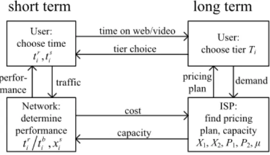
On a time scale of days, broadband Internet subscribers choose how much time to devote to Internet applications, presumably by evaluating their willingness-to-pay based on the utility accrued through their use of these applications. However, the tier design determines the performance of the applications, which in turn affects user decisions about the time spent on the applications. Performance and time will further affect user decisions about tier subscription in return, as illustrated in Fig. 1. We thus investigate these relationships in section III.

User: choose time short term Network: determine performance User: choose tier Ti ISP: find pricing plan, capacity X1, X2, P1, P2, μ perfor-mance traffic capacity cost demand pricing plan tier choice time on web/video long term , r s i i t t , r b s i i i t t x

Figure 1. Relationships among an ISP and its subscribers.

We focus on the bottleneck link within the access network. Denote by λ (in bits per month) the total downstream traffic for subscribers within the access network. This aggregate downstream traffic is simply the sum of demands by each user:

b b s s i i i i i L t r x t M

λ

= _ + _  

∑

(7)

where L is the average size (in bits) of a web page and M is the average time (in seconds) spent on reading a web page. As is common, we model the bottleneck link using an M/M/1/K queue to estimate the average delay d and loss l as a function of the traffic λ and the capacity μ.

It remains to express the dependence of application performance upon delay and loss. Suppose that user i has subscribed to tier j and thereby obtains a tier rate Xj. For web

browsing, utility depends on performance through a function

( )

b r i

V t that measures the relative value of time devoted to reading web pages. The ratio of time spent reading web pages to time spent web browsing, b r b

i i i

r =t t , can be derived from a TCP latency model [18]; we denote it as a function TCPb _{of the}

access network delay d, access network loss l, and the user’s tier rate Xj:

(

, ,

)

b r b b

i i i j

r =t t =TCP d l X (8)

For video streaming, utility depends on performance through a sigmoid function s

( )

s

i

Q x of the throughput s i

x

experienced by video streaming applications. Most video streaming uses TCP or TCP-friendly protocols and the throughput can be derived from similar TCP models [19]; we denote it as a function TCPs _{of the access network delay d,}

access network loss l, and the user’s tier rate Xj:

(

, ,

)

s s

i j

x =TCP d l X (9)

III. DEMAND FUNCTION

In the United States and many other countries, it is common that only one or two ISPs offer wireline broadband service [2]. In the remainder of the paper, we consider one ISP that monopolizes the market. Since the current academic literature similarly analyzes a monopoly provider, and here our goal is to extend those models by considering two classes of applications and the time that users devote to each, a monopoly model is a reasonable starting point.

To derive the monopolist’s demand function that expresses the dependence of user tier subscriptions upon prices and performance, we presume that (1) in the short term model users choose the time spent on web browsing and video streaming by maximizing willingness-to-pay, and (2) in the long term users choose whether to subscribe to broadband Internet access and if so which tier to subscribe to.

Denote user i’s willingness-to-pay if they have subscribed to tier j by

(

b, |s

)

i i i

W t t j . Denote the ratio of time spent reading web pages by users in tier j by rb,j_{, and the throughput of video}

streaming by users in tier j by xs,j_{. Using (1), (2), (4), and (5),}

(

b, |s

)

i i i

W t t j can be expressed as a function of

(

b, ,s t

)

i i i v v p :

(

b_{, , |}s t

)

b b

( )

b j b, t b s s

( ) ( )

s s s j, t s i i i i i i i i i i i i W v v p j v V r t= −p t v V t Q x+ −p t (10) where b i t and s i

t can be obtained from (5) given performance rb,j

and xs,j _{in tier j.}

Denote user i’s tier choice by Ti = 0,1,2, where Ti = 0 means

that user i chooses not to subscribe. The values of

(

b, ,s t

)

i i i

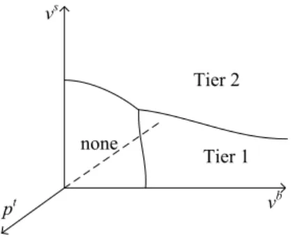
v v p determine a user’s choice of tiers, as shown in Fig. 2. User i will choose tier Ti iff:

(

)

arg max b, , |s t

i _j i i i i j

T = _W v v p j −P_.

If there is competition between multiple ISPs, then a user would also have to choose between different tiers offered by multiple ISPs. Tier 1 Tier 2 none vb vs pt

Figure 2. Users subscribe to tier 1 service, tier 2 service or nothing. Denote the total number of users in the market by N. Denote the set of users that subscribe to tier j by

(

)

{

b, ,s t such that

}

j i i i i

S = v v p T = j , and the number of users

that subscribe to tier j by Nj = | Sj |. Denote the distribution in

the market of users’ relative utilities for web browsing and video streaming and their opportunity cost of time by a density function f(vb_{, v}s_{, p}t_{). The demand function for each tier is given}

by:

(

)

(

, ,

)

, , b s t b s _j t b s t j _{v v p S} N N f v v p dv dv dp ∈ =

∫

(11)

According to (7), the aggregate traffic in the network can be calculated as follows:

(

)

(

)

, , , , , , , , b s t j b j b j b s t s j s j b s t j v v p S t r L Nf v v p x t dv dv dp M λ ∈   = _ + _  

∑ ∫

(12)

where tb,j _{and t}s,j _{are the amount of time users with (v}b_{, v}s_{, p}t₎

spent on web browsing and video streaming in tier j. They can be obtained from (5). Note that the performance rb,1_{, r}b,2_{, x}s,1_, and xs,2 _{of each tier depends on the tier rates X1, X2, network} loss l and network delay d. Furthermore, the loss l and delay d

depend on the traffic rate λ using the M/M/1/K network model. Thus rb,1_{, r}b,2_{, x}s,1_{, and x}s,2 _{can be expressed as functions of λ,} and (12) is thus a nonlinear fixed point equation in λ.

IV. ISP TIER DESIGN

In the previous two sections, we introduced utility functions for web browsing and video streaming, and derived user demand for each tier. In this section, we seek to understand how an ISP may design a tiered pricing plan and bottleneck network capacity. ISP methods for tier design are proprietary; however, an understanding of how an ISP may approach tier design is essential for networking research. Our model can provide insight into this problem, by naturally decomposing the

network capacity and tier design problem into three sub-problems for the ISP engineering and marketing departments. Given the density function f(vb_{, v}s_{, p}t_{), the relative value}

functions Vs_(ts_{), V}b_(tb_{), the video streaming performance}

function Qs_(xs_{), and an accurate network model, an ISP could}

calculate the optimal tiered pricing plan P1, P2, X1, X2 and network capacity μ so as to maximize its profit, denoted by

Profit=P1N1+P2N2−C(μ). The first order conditions for optimality are:

(

)

1 , 2 , 1 , 2 , 0, 0, 0, 0, 0

Profit Profit Profit Profit Profit

P P X X ρ

∂ ∂ ∂ ∂ ∂ ₌

 _{∂ ∂ ∂ ∂ ∂} 

  (13)

However, it is difficult for an ISP to directly calculate the optimal pricing plan and network capacity from (13). First, an ISP may not have complete knowledge of all of the required functions. Second, an ISP may find it challenging to instill the required cooperation between its engineering department, which is traditionally focused on network architecture and performance, and its marketing department, which is traditionally focused on pricing and demand. Thus, it is natural for an ISP to attempt to decompose the task of profit maximization between its engineering and marketing departments.

A.Engineering department determination of network capacity

An ISP’s engineering department typically has the primary responsibility for determining network capacity. While we are not privy to proprietary information about the operation of ISPs, our understanding is that many use a dimensioning rule of thumb: a capacity upgrade is scheduled when the load on a network link exceeds a threshold1_{, here denoted by ρ}th_{. Thus,}

given network traffic λ during the peak time period, an ISP’s engineering department may invest so that network capacity μ satisfies:

th

ρ λ µ ρ= ≤ (14)

We ask here whether such a rule of thumb applied to the capacity μ of the bottleneck link effectively maximizes profit. Denote the marginal network cost by pμ_{=dC(μ)/dμ. The optimal}

choice for ρ would result in:

,1 ,2 1,2 1,2 ,1 ,2 ,1 ,2 1,2 1,2 ,1 ,2 2 1 0 b b j j j j j j b b s s j j j j j j s s P N P N Profit r r r r P N _x P N _x p x x µ ρ ρ ρ λ λ ρ ρ ρ ρ ρ = = = = ∂ ∂ ∂ ₌ ∂ ₊ ∂ ₊ ∂ ∂ ∂ ∂ ∂ ∂ _∂ ∂ _{∂  ∂ } + − _ − _ ∂ ∂ ∂ ∂ ∂ _{ } =

∑

∑

∑

∑

₍₁₅₎

Web browsing performance in both tiers, rb,1 _{and r}b,2_, deteriorates with network load ρ. Similarly, video streaming performance in tier 2, xs,2_{, deteriorates with network load ρ.} However, video streaming performance in tier 1, xs,1_{, would} likely not change with network load ρ, since it would likely be constrained by tier rate X1. As a result, any increase in load ρ

1 _{A commonly discussed choice for ρ}th _{is 0.7.}

4

will result in users spending less time on both applications, and the total traffic λ will fall. Thus:

,1 ,2 ,1 ,2 0, 0, 0, 0, 0 b b s s r r x x λ ρ ρ ρ ρ ρ ∂ ∂ ∂ ∂ ∂ ≤ ≤ ≈ ≤ ≤ ∂ ∂ ∂ ∂ ∂

The magnitude of these terms, however, depends on the load ρ. The dimensioning rule of thumb was based on observations that web browsing performance is good when loads are below a threshold, but begins to deteriorate quickly at loads above that threshold. With the increasing popularity of video streaming, ISPs seem to be using a similar rule of thumb for video streaming, but with a lower threshold. Thus, we conjecture that use of the dimensioning rule of thumb results in ∂rb,1_{/∂ρ≈0,∂r}b,2_{/∂ρ≈0,∂x}s,2_{/∂ρ≈0 when ρ<ρ}th_{, and ∂r}b,1_{/∂ρ <0,}

∂rb,2_{/∂ρ<0, ∂x}s,2_{/∂ρ<0 when ρ>ρ}th_{. The last term in (15) is a}

large positive number when ρ<ρth_{, and is a small positive}

number when ρ>ρth_{. Thus ∂Profit/∂ρis a large positive number}

when ρ<ρth_{, is near 0 when ρ≈ρ}th_{, and is negative when ρ>ρ}th_.

Thus, it appears to be near optimal for an ISP to maintain a network load ρ slightly smaller than ρth_{. We expect that the}

amount of sub-optimality will depend on the choice of the threshold ρth _{and upon how quickly the performance of web}

browsing and video streaming change when the load exceeds the threshold. We will investigate this in section V.

B.Marketing department determination of tier price

An ISP’s marketing department typically has the primary responsibility for determining tier prices. While we are not privy to proprietary information about how they approach this task, we expect that they attempt to maximize profit. We presume here that the marketing department takes into account the engineering department’s dimensioning rule of thumb, namely they assume that μ = λ/ρth_{. Given this dependence, the}

optimal choices for P1and P2would result in:

1 2 1 2 0 j _th j j j j N N Profit _{N P P} p P P P P µ _λ ρ ∂ ∂ ∂ _{= + + −} ∂ ₌ ∂ ∂ ∂ ∂ (16)

If the ISP has estimated the market density f(vb_{, v}s_{, p}t_{), then}

it can estimate the sensitivities of demands with prices {∂N1/∂Pj,

∂N2/∂Pj}from the demand functions in (11). In this case, it will

likely consider the performance of web browsing and video streaming {rb,1_{, r}b,2_{, x}s,1_{, x}s,2_{} as fixed, i.e. estimate {dN1/dPj,}

dN2/dPj} instead of {∂N1/∂Pj, ∂N2/∂Pj}, since the dimensioning

rule of thumb should keep the network load constant. Alternatively, we observe that some ISPs directly estimate these sensitivities from market surveys and/or pricing tests.

The last term in (16) is the impact of the tier prices on the network cost. Similarly, if the ISP has estimated the market density f(vb_{, v}s_{, p}t_{) and knows the time that users devote to web}

browsing and video streaming, then it can estimate the sensitivities of traffic with prices {∂λ/∂Pj} from (12), now

holding both the performance of web browsing and video streaming and the time devoted to each {tb,j_{, t}s,j_{} as fixed.}

Alternatively, if ISP directly estimates the sensitivities of demands with prices, it may also directly estimate the sensitivities of traffic with prices.

Thus, the marketing department may attempt to maximize profit by selecting tier prices {P1,P2} using (16). However, these prices will not be optimal since, through its reliance on

the dimensioning rule of thumb, it presumes that optimal performance does not vary with price. We will investigate the amount of sub-optimality in section V.

C.Joint determination of tier rates

We have presumed above that an ISP’s engineering department is tasked with determining network capacity and that an ISP’s marketing department is tasked with determining tier prices. The remaining task is that of determining tier rates {X1, X2}. We are unsure of how most ISPs handle this task. Tier rates affect the performance of web browsing and video streaming, and thus affect users’ willingness-to-pay through (10). This in turn affects both the demand for each tier through (11) and the network traffic through (12). We conjecture that ISPs thus must involve both their engineering and marketing departments in this task.

Choosing tier rates to satisfy ∂Profit/∂X1=0 and

∂Profit/∂X2=0 appears to us to be too complex of a task to be undertaken directly by an ISP.Thus, we address determination of the rate for each tier separately in the following two subsections.

1)Determination of tier 1 rate

Given the use of a dimensioning rule of thumb, the choice of X1 should have little effect upon the performance of web browsing and video streaming in tier 2. Similarly, the choice of

X2 should have little effect upon the performance of web browsing and video streaming in tier 1. Thus, we assume that:

,1 ,1 ,2 ,2 2 2 1 1 0, 0, 0, 0 b s b s r x r x X X X X ∂ _≈ ∂ _≈ ∂ _≈ ∂ _≈ ∂ ∂ ∂ ∂

The partial derivative of profit with respect to tier 1 rate can then be simplified to:

( )

( )

( )

( )

,1 ,1 1 1 1 _{,1 ,1} 1 1 1 ,1 ,1 2 2 2 _{,1 ,1} 1 1 1 s s b b s s s s b b s s th Q x N N Profit _P r X r X Q x X Q x N r N p P X X X r Q x µ _λ ρ  _{∂ ∂ ∂}  ∂ _ ∂ _ = _ + _ ∂ _∂ ∂ ∂ ∂ _ _{∂ ∂ ∂ ∂}  _∂   + _ + _− ∂ ∂ ∂ ∂  ∂   

and the partial derivative of λwith respect to tier 1 rate can be simplified to:

( )

( )

,1 ,1 ,1 ,1 1 1 1 s s b b s s Q x r X r X Q x X λ λ λ ∂ ∂ ∂ ∂ ∂ = + ∂ ∂ ∂ ∂ ∂

The throughput of video streaming in tier 1, xs,1_{, is very likely} to be constrained by tier rate X1, leading to xs,1 = X1. The quality of web browsing, rb,1_{, is an increasing concave function} of X1, while the quality of video streaming Qs(xs,1) is a sigmoid function of X1. On this basis, we make the following conjecture:

Conjecture A: There exists an interval X1_≥X1≥X0_{, where the} quality of web browsing rb _{is very good, but the quality of}

video streaming Qs_(xs_{) is not desirable.}

Conjecture A is based on the common observation that the minimum required tier rate X1 _{for decent video streaming is} larger than that of web browsing, i.e. X0_{. According to Fig. 4,}

Qs _{has two flat portions. The initial flat portion (X}1_≥X1) corresponds to poor video streaming performance under a low tier rate, where ∂Qs_(xs,1_{)/∂X1≈ 0. Similarly, r}b _{also has a flat}

portion (X1≥X0) corresponding to good web browsing, where

∂rb,1_{/∂X1≈ 0.}

Thus, we can make the following approximations, when

X1_≥X1≥X0_:

( )

,1 ,1 1 0, 1 0 1 0 s s b Q x r Profit X X X ∂ ∂ ∂ ≈ ≈ ⇒ ≈ ∂ ∂ ∂

Thus, any choice of X1 within X1≥X1≥X0 can approximately maximize profit. One reasonable choice for X1 is:

1

X =Win RTT (17)

where Win is the maximum TCP receive window size and RTT

denotes a typical round trip time.

The determination of tier 1 rate can thus be accomplished entirely by the engineering department. The amount of sub-optimality introduced by these approximations will largely depend upon the shape of the functions rb,1_{(X1) and Q}s_(X1),

which we will investigate in section V.

2)Determination of tier 2 rate

The determination of tier 2 rate is more complex, and we believe it will involve both the engineering and marketing departments. Using the approximations given in the previous subsection, the partial derivative of profit with respect to tier 2 rate can be simplified to:

1 2 1 2 2 2 2 th 2 N N Profit _{P P} p X X X X µ _λ ρ ∂ ∂ ∂ _{= + −} ∂ ∂ ∂ ∂ ∂ (18)

We presume here that determination of tier rates occurs after network capacity and tier prices have been determined as outlined above. The throughput of video streaming in tier 2, xs,2_, is very likely to be constrained by tier rate X2, leading to xs,2 =

X2.

The partial derivatives of demand and traffic to tier 2 rate, however, depend on many factors. Define user Internet surplus as the willingness-to-pay minus the paid tier price. Denote by

Sj,k the set of users with equal surplus in tier j and tier k (i.e. the

users in Fig. 2 on the boundary between two regions). We propose two additional conjectures solely to simplify estimation of ∂Profit/∂X2:

Conjecture B: | S0,2| << | S1,2|.

Conjecture B is based on the common observation that most marginal users in tier 2 prefer tier 1 to no Internet subscription. Conjecture C: t t

i

p = p i∀ .

Conjecture C assumes that all users place the same value pt _on

their time. We let pt _{be the average value among all} t i

p , when calculating the near-optimal tier 2 rate.

Theorem: Based on these conjectures, ∂Profit/∂X2 can be approximated as follows:

( )

( )

( )

( )

( )

( )

,2 ,2 2 2 2 ,2 2 2 ,2 2 2 _,2 2 s s s s mar mar s s s s th _{th s s} s Profit N v V t Q X X p N Q X V t p N t X Q X V t µ µ ρ _ρ ′ ∂ _′ ≈ ∂ ′ − + ′′ (19) where, s,2

(

s| 2

)

i i

t =E t T = is the average amount of time users

in tier 2 spend on video streaming, ,2

(

)

1,2 |

s s

mar i

t =E t i S∈ is the

average time users indifferent to tiers 1 and 2 spend on video streaming, and vmars,2 =E v i S

(

is| ∈ 1,2

)

is the average relative value placed on video streaming by users indifferent to tiers 1 and 2.

Proof: See Appendix.

The first term in (19) can be interpreted as the marginal revenue produced by an increase in tier 2 rate, if the price of tier 2 is simultaneously increased by the amount that leaves the number of subscribers to tier 2 unchanged. The second term can be interpreted as the marginal cost for capacity produced by an increase in tier 2 rate required accommodating the increased transmission rate for video streaming. The third term can be interpreted as the marginal cost for capacity produced by an increase in tier 2 rate required accommodating the increased time spent on video streaming due to an increase in quality of video streaming.

The determination of tier 2 rate can be calculated from (19) by setting ∂Profit/∂X2 equal to zero. The engineering department would likely have knowledge of Qs_{, dQ}s_{/dX2, p}μ_,

and ts,2 , the marketing department would likely have knowledge of pt_{, V}s _{and its derivatives, and both departments}

must cooperate to estimate ∂Profit/∂X2. The amount of sub-optimality introduced by these approximations will largely depend upon the validity of Conjecture C, which we will investigate in section V.

V. NUMERICAL RESULTS

In this section, we explore the magnitude of the decrease in profit resulting from the various sources of sub-optimality discussed in the previous section, and the variation of the design with key parameters. We do not compare these designs to other designs, since the current academic literature does not consider two classes of applications nor the time users devote to applications, and are thus not comparable.

A.Magnitude of sub-optimality

The use of a dimensioning rule of thumb, based on the presumption of a threshold ρth_{, may cause significant}

sub-optimality. To investigate this, parameters are set as follows:

L=750KB [21]; 10 concurrent TCP connections for web browsing; TCP packet size = 512B; RTT=100ms; M/M/1/K service rate = 600Mbps and buffer size = 25, 50, or 100 packets; video streaming service based on TCP with Qs_(xs_{) as in [22].}

Fig. 3 shows the performance of web browsing and video streaming as a function of network load. For a 50 packet buffer, there is a fairly steep decline in performance of web browsing when ρ>0.97, and in the performance of video streaming when ρ>0.87. Fig. 4 shows the performance of web browsing and video streaming as a function of access tier rate for a 50 packet buffer when ρ=0.7. The performance of web browsing is a concave function of the tier rate, and is fairly constant for

X>2.5Mbps. The performance of video streaming is a sigmoid function of the tier rate; it is fairly constant at poor performance when X<3Mbps, rises quickly for 3Mbps<X<18Mbps, and is fairly constant at high performance when X>18Mbps. Thus,

although both web browsing and video streaming performance experience a sharp threshold with respect to load, there is much slower change in video streaming performance.

0.0 0.2 0.4 0.6 0.8 1.0 0.5 0.6 0.7 0.8 0.9 1.0 Q ual ity of br ow sing/ st ream ing Network load browsing, 25pks streaming, 25pkts browsing, 50pkts streaming, 50pkts browsing, 100pkts streaming, 100pkts

Figure 3. The dependence of performance rb _{and Q}s _{upon network load ρ.}

0 5 10 15 20 25 0.0 0.1 0.2 0.3 0.4 0.5 0.6 0.7 0.8 0.9 1.0 Q ual ity of Int er net appl icat ions Tier rate (Mbps) web browsing video streaming

Figure 4. The dependence of performance rb _{and Q}s _{on the tier rate.}

To gauge the size of this source of sub-optimality, we compare the optimal choices of capacity, tier prices, and tier rates to those chosen, using the simplified scheme under the following parameters: Vb_(tb_{) = log(abt}b _{+ 1) with ab = 0.0026,}

so that a user with tb_{=50 hours/month [23] is willing to pay $60}

for tier 1 [24]; Vs_(ts_{) = log(ast}s _{+ 1), with as = 0.0093, so that a}

user with ts_{=15 hours/month [25] is willing to pay an additional}

$20 to move from tier 1 to tier 2 [24]; N=20000; (vb_{, v}s_{, p}t_{) ~}

multivariate lognormal with (vb_/pt_{, v}s_/pt_{)independent of p}t_{, fp(p}t₎

given by 2009 US household income [26], f(vb_/pt_{) given by}

[23], f(vs_/pt_{) given by [25], and the correlation between v}b_/pt

and vs_/pt _{= 0.5; p}μ_{= $10/Mbps/month [27]; peak traffic = 1.55}

times average traffic [12]; buffer = 50 packets; ρth _{= 0.7.}

Table 1 presents the parameters and profits of the optimal design (13) and the simplified design. The designs match fairly closely, but the simplified design results in 4.3% less profit.

TABLE I. NEAR-OPTIMAL RESULTS AND OPTIMAL RESULTS Simplified Optimal Price of tier 1 P1 $68 $65 Price of tier 2 P2 $84 $80 Rate of tier 1 X1 2.5Mbps 2.5Mbps Rate of tier 2 X2 20Mbps 22.2Mbps Network capacity μ 6.31Gbps 6.41Gbps Profit $371600 $388280

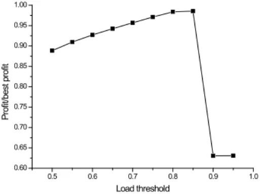
Fig. 5 shows the percentage of the optimal profit that the simplified design achieves under different load thresholds ρth_.

We observe profit increases with ρth _{until ρ}th _{= 0.85, when the}

simplified scheme achieves 98.5% of optimal, and then falls quickly after that. The optimal value of ρth _{= 0.85 corresponds}

to the load threshold for video streaming as seen in Fig. 3.

0.5 0.6 0.7 0.8 0.9 1.0 0.60 0.65 0.70 0.75 0.80 0.85 0.90 0.95 1.00 Pr of it/ bes t pr of it Load threshold

Figure 5. Sub-optimal profit over optimal profit under different ρth_.

The dimensioning rule of thumb is the largest source of sub-optimality in the numerical results in this section, and the choice of the threshold is the most significant factor. The determination of tier prices contributes additional sub-optimality through its reliance on the dimensioning rule of thumb, which presumes that optimal performance does not vary with price. The determination of tier rates contributes additional sub-optimality through approximations, which depend upon the shape of the functions rb,1_{(X1)and Q}s_{(X1) and}

upon the validity of Conjecture C. In numerical results, these contributions are minor.

B.Variation of the design with key parameters

In this final subsection, we explore the variation of the simplified design with key parameters. Fig. 6 shows the dependence of profit upon the marginal network cost pμ_.

Unsurprisingly, the cost of capacity decreases and profit increases as marginal network cost decreases.

The impact upon the demand for each tier is complex. First, consider the impact of pμ _{on tier prices. The marketing}

department considers whether to increase or decrease P1 in response. If it increases P1, this will result in users in S0,1 dropping service, with a small decrease in traffic, and users in

S1,2 upgrading from tier 1 to tier 2, with a substantial increase in

traffic. As a result, ∂λ/∂P1>0 and when pμ decreases,

∂Profit/∂P1 becomes positive from (16). Thus, the ISP will increase P1 to earn more profit. The marketing department will then consider whether to modify P2. If it increases P2, this will result in users in S1,2 downgrading from tier 2 to tier 1, with a

substantial decrease in traffic. As a result, ∂λ/∂P2<0, and when

pμ _{decreases, ∂Profit/∂P2 becomes negative from (16). Thus,}

the ISP will decrease P2 to earn more profit.

Next consider the impact upon tier rates. Tier 1 rate is set by the engineering department using (17) which does not depend upon pμ_{. The engineering and marketing departments}

jointly use (19) to set tier 2 rate; decreasing pμ _makes ∂Profit/∂X2 positive, and thus the ISP will increase tier rate X2.

Since the price of tier 2 has decreased while tier 2 rate has increased, the demand for tier 2 will increase. The increase in tier 2 demand outweighs the decrease in tier 2 price, and thus revenue from tier 2 increases. Similarly, the price of tier 1 has increased, causing users to upgrade to tier 2 and causing revenue from tier 1 to decrease.

22 20 18 16 14 12 10 8 6 4 2 0 1.2x105 1.4x105 1.6x105 1.8x105 2.0x105 2.2x105 2.4x105 2.6x105 2.8x105 3.0x105 3.2x105 3.4x105 3.6x105 3.8x105 4.0x105 4.2x105 4.4x105 4.6x105 IS P pr of it/ rev enue ( $)

Network cost ($/Mbps/month) ISP profit

Revenue from tier 1 Revenue from tier 2

Figure 6. The dependence of profit upon the marginal network cost pμ_.

Finally, we explore the effect of increasing video streaming popularity. To investigate this, we simultaneously increase vb

and decrease the parameter as in Vs(ts), so that the average

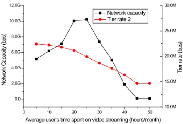
user’s time spent on video streaming increases but their willingness-to-pay for streaming remains unchanged. Fig. 7 shows the network capacity and tier 2 rate as a function of the average user’s time spent on video streaming.

As users devote more time to video streaming, ∂Profit/∂X2 becomes negative, and thus the engineering and marketing departments will jointly reduce tier rate X2 using (19). This will cause some users to downgrade from tier 2 to tier 1.

0 10 20 30 40 50 0.0 2.0G 4.0G 6.0G 8.0G 10.0G 12.0G 10.0M 15.0M 20.0M 25.0M 30.0M Ti er rat e ( bps ) Network capacity Net wor k C apac ity (bps )

Average user's time spent on video streaming (hours/month) Tier rate 2

Figure 7. Network capacity and tier 2 rate vs. video streaming time. The effect on traffic is more complex. For small increases in the average streaming time, the increase in video streaming time by those who remain in tier 2 outweighs the very small reduction in tier 2 subscriptions and performance, and hence results in an increase in traffic. As a result, the engineering department increases capacity μ according to (14). However, for larger increases in video streaming time, the tier 2 subscriptions and performance begin to drop quickly, outweighing the increase in video streaming time by those who

remain in tier 2, and hence resulting in a decrease in traffic, and thus a decrease in capacity.

VI. CONCLUSION

We proposed a model of how an ISP may set tier prices, tier rates, and network capacity by considering both technical and economic issues. Web browsing and video streaming are modeled by utility functions depending on performance, devoted time, user’s valuation of time and of applications, instead of only an aggregated service quality (e.g. bandwidth). A general cost function depending on the network capacity is used, instead of assuming a fixed cost per user. On a time scale of days, users choose how much time to devote to applications based on the opportunity cost of their time. On a time scale of months, ISPs choose tier rates and prices, and users make subscriptions decisions.

For a monopoly ISP, we derived demand as a function of tier price and performance, and conditions for the optimal tiered pricing plan and network capacity. We then use our model to answer how ISPs may design tiered pricing plans, which is proprietary but important to networking research. Model analysis shows that the complex ISP profit maximization problem can be decomposed by the ISP, where the engineering department sets network capacity, the marketing department sets tier prices, and they jointly set tier rates. Numerical results are presented to illustrate the magnitude of the decrease in profit resulting from such a possible design taken by the ISPs. Although ISPs’ approaches to these tasks are proprietary, we hope that this model may support research that depends on an understanding of tier designs.

We believe this is the first model presented in the academic literature of how an ISP may design tier rates, tier prices, and network capacity that considers two classes of applications or the time users devote to applications. Although the monopoly case is interesting in its own right, an excellent topic for future research would be consideration of market demand and tier design when there are multiple ISPs competing in a market.

VII.APPENDIX Proof of theorem: Using Conjecture A: ,1 ,1 ,2 ,1 ,2 ,1 ,2 ,1 2 2 2 0, 0, 0, , , 0 s b b b b b b s

mar mar mar

x r r _{r r t t t} X X X ∂ _≈ ∂ _≈ ∂ _{≈ ≈ ≈ ≈} ∂ ∂ ∂ where b,1 mar t and b,2 mar t (resp. s,1 mar t _and s,2 mar

t ) are the average times users in S1,2, and in tiers 1 and 2 respectively, spend on web browsing (resp. video streaming). Thus, when xs,2 _is constrained by tier rate X2:

,2 _{,2 ,2} ,2 _,2 2 2 2 2 2 2 2 2 s _{b b} s _{mar s} mar t r L N t N X t t X X X X M λ     ∂ _{≈ } ∂ _{+ +}∂ ₊       ∂ _ ∂ _ ∂ _{ }

The first term gives the marginal traffic of current tier 2 users resulting from increased transmission rates and from additional time devoted to video streaming due to improved performance. The second term gives the marginal traffic due to new tier 2 subscribers.

By considering the performances in tier 1 as independent of tier rate X2:

,1 ,1 ,1 ,1 ,1 ,1 1 1 1 2 2 2 b b b b s s mar mar mar t r L t r L N _{t x} N X X M X M λ   ∂ ∂ ∂ ≈ _ + _≈ ∂ ∂ _{ } ∂

Using Conjecture B, a marginal increase in X2 primarily

causes some marginal users to upgrade from tier 1 to tier 2, with the total number of subscribers remaining constant:

(

1 2

)

1 2 2 0 2 2 N N N N X X X ∂ + ∂ ∂ ≈ ⇒ = − ∂ ∂ ∂

Thus, we have the following approximations for ∂λ/∂X2:

(

)

,2 ,2 1 2 2 ,2 2 2 2 2 2 2 2 s s _s mar N t N X t t X X X X X λ λ λ ∂ +   ∂ ∂ _ ∂ _ = ≈ + +   ∂ ∂ ∂ ∂  

It remains to find expressions for ∂N2/∂X2 and ,2 2

s

t X

∂ ∂ to get an expression for ∂Profit/∂X2 in (18). We presumed that tier prices have already been determined according to (16). Thus:

,2 2 2 2 2 1 2 0 2 s mar th N p X t Profit _{N P P} P P µ ρ   ∂ ∂ = ⇒ = − _ − − _ ∂ ∂ _{ }

An increase in tier 2 rate will increase such marginal users’ willingness-to-pay for video streaming in tier 2. Thus:

(

)

(

)

(

)

(

)

( )

( )

,2 2 2 1 2 2 ,2 ,2 2 2 2 1 2 ,2 ,2 2 2 2 1 2 ,2 ,2 _,2 2 1 2 2 ,2 2 2 2 ,2 ,2 ,2 2 2 2 2 2 2 Prob Prob Prob Prob s s s s s mar s s _s mar _mar s mar s s s s s mar mar mar N _{N W P P X} X N W X W X P P X N W X W X P P X N W P P X W X _W X X W X W N _{N v V t Q X} P X P ∂ ≈ ∂ > − ∂ ∂ = + ∆ ∂ ∂ > − ∆ = + ∆ ∂ ∂ > − ∆ > − − ∆ ∂ ∂ _∂ = ∂ ∆ ∂ ∂ ∂ ∂ ∂ _′ = − = − ∂ ∂ ∂

Using Conjecture C, the average time users in tier 2 spend on video streaming can be estimated from (5) using:

( )

( )

( )

,2 ,2 ,2 1 2 _,2 2 t s s s s s t s s ps v V t Q X p t V v Q X −   ′ = ⇒ = _{′ } _  

Thus, given pt _{and v}s,2_, ,2 2

s

t X

∂ ∂ can be expressed as:

( )

( )

( )

( )

( )

,2 ,2 ₂ 1 2 ,2 ,2 2 2 ₂ s s s s _t s s s _{s s} s Q X V t t _V p _X X v Q X _{Q X V t} ′ − ′   ∂ _{= ∂ ′   ∂ = −}   ∂ _{  ′′}

Thus, we can derive the final expression for ∂Profit/∂X2 in (19) by replacing ∂λ/∂X2, ∂N2/∂X2 and ∂ts,2 ∂X2in (18).

REFERENCES

[1] AT&T, “U-Verse pricing”, http://www.att.com/u-verse/shop/, accessed Apr. 30, 2012.

[2] Cox Communications, “Cox Internet pricing”,

http://ww2.cox.com/residential/internet.cox, accessed Apr. 30 2012. [3] A. Gold and C. Hogendorn, “Tipping in two-sided markets with

asymmetric platforms,” Telecommunications Policy Research Conference, 2011.

[4] J. Musacchio and D. Kim, “Network platform competition in a two-sided market: Implications to the net neutrality issue,”

Telecommunications Policy Research Conference, 2009. [5] M. Chiang et al., “Pricing broadband: Survey and open problems,”

Second International Conference on Ubiquitous and Future Networks (ICUFN), 2010.

[6] P. Hande et al., “Pricing under constraints in access networks: Revenue maximization and congestion management,” IEEE Infocom, Mar. 2010. [7] S. Shakkottai et al., “The price of simplicity,” IEEE Journal on Selected

Areas in Communications, vol. 26, no. 7, pp. 1269-1276, Sep. 2008. [8] Linhai He and Jean Walrand, “Pricing differentiated Internet services,”

IEEE Infocom, Mar. 2005.

[9] Qian Lv and George N. Rouskas, “An Economic Model for Pricing Tiered Network Services,” IEEE ICC 2009.

[10] Qian Lv and George N. Rouskas, “Internet Service Tiering as a Market Segmentation Strategy,” IEEE GLOBECOM 2009.

[11] Sandvine Incorporated, “Global Internet phenomena report 2012,”

Technical report, Fall 2012.

[12] Yong Liu, Yang Guo, Chao Liang, “A survey on peer-to-peer video streaming systems,” Peer-to-Peer Networking and Applications, vol. 1, no. 1, Mar. 2008.

[13] W. Wang, M. Palaniswami, and S. H. Low, “Application-oriented flow control: Fundamentals, algorithms and fairness,” IEEE/ACM Transaction on Networking, vol. 14, no.6, pp. 1282–1291, Dec. 2006. [14] John Musacchio, Jean Walrand, “WiFi Access Point Pricing as a

Dynamic Game,” IEEE/ACM Transactions on Networking, vol. 14, no. 2, pp. 289-301, Apr. 2006.

[15] Hans U Gerber, Gerard Pafumi, “Utility Functions: From Risk Theory to Finance,” North American Actuarial Journal, Jul. 1998.

[16] O. Ormond, J. Murphy, and G.-M. Muntean, “Utility-based intelligent network selection in beyond 3G systems,” IEEE International Conference on Communications(ICC), 2006.

[17] P. Hande, Z. Shengyu, and C. Mung, “Distributed rate allocation for inelastic flows,” IEEE/ACM Transaction on Networking, vol. 15, no.6, pp. 1240–1253, Dec. 2007.

[18] N. Cardwell, S. Savage, and T. Anderson, “Modeling TCP latency,”

IEEE Infocom, pp. 1742-1751, Mar. 2000.

[19] J. Padhye, V. Firoiu, D. Towsley, and J. Kurose, “Modeling TCP throughput: A simple model and its empirical validation,” ACM SIGCOMM, 1998.

[20] Nicholas Economides, “Net Neutrality, Non-Discrimination and Digital Distribution of Content Through the Internet,” Journal of Law and Policy for the Information Society, vol. 4, no. 2, 2008.

[21] Website Optimization LLC, “Average web page size septuples since 2003,” http://www.websiteoptimization.com/speed/tweak/averageweb-page/, accessed April 30th, 2012.

[22] S. Weber and V. Veeraraghavan, “Distributed algorithms for rate-adaptive media streams,” INFORMS Telecommunications Conference, Dec. 2007.

[23] Georgia Tech Research Corporation, “GVN's 10th WWW user survey,” 1998, available at http://www.cc.gatech.edu/gvu/user_surveys/survey-1998-10/graphs/use/q02.htm.

[24] G. Rosston, S. Savage, and D. Waldman, “Household demand for broadband Internet service,” Final report to the Broadband.gov Task Force Federal Communications Commission, Feb. 3, 2010.

[25] Burstmedia.com, “Online video content & advertising video preferences, habits and actions in Q4 2011,” Oct. 2011, available at

http://www.burstmedia.com/pdf/burst_media_online_insights_2011_11. pdf.

[26] United States Census Bureau, “Money income of households, 2009,” 2009, available at

http://www.census.gov/compendia/statab/2012/tables/12s0690.pdf [27] CCS Leeds Network Solutions, “UK leased lines pricing,”

http://www.uk-leased-line.co.uk/prices.html, accessed Apr.30 2012.