CIRJE Discussion Papers can be downloaded without charge from: http://www.e.u-tokyo.ac.jp/cirje/research/03research02dp.html
Discussion Papers are a series of manuscripts in their draft form. They are not intended for circulation or distribution except as indicated by the author. For that reason Discussion Papers may
CIRJE-F-733
Robustness of the Separating Information
Maximum Likelihood Estimation of the Realized
Volatility with Micro-Market Noise
Naoto Kunitomo University of Tokyo
Seisho Sato
Institute of Statistical Mathematics April 2010
Robustness of the Separating Information
Maximum Likelihood Estimation of the Realized
Volatility with Micro-Market Noise
∗
Naoto Kunitomo
†and
Seisho Sato
‡April 10, 2010
Abstract
For estimating the realized volatility and covariance by using high frequency data, Kunitomo and Sato (2008a,b) have proposed the Separating Information Maximum Likelihood (SIML) method when there are micro-market noises. The SIML estimator has reasonable asymptotic properties; it is consistent and it has the asymptotic normality (or the stable convergence in the general case) when the sample size is large under general conditions includingnon-Gaussian processesand
volatility models. We also show that the SIML estimator has the asymptotic robustness in the sense that it is consistent and it has the asymptotic normality when there are autocorrelations in the market noise terms and there are endogenous correlations between the signal and noise terms.
Key Words
Realized Volatility with Micro-Market Noise, High-Frequency Data, Separating Information Max-imum Likelihood (SIML), Endogenous Noise, Autocorrelated Noise, Robustness.
∗KSIII-10-4-10-2. An eariler version of this paper was presented at a conference on financial
econometrics held at the University of Tokyo in March 30, 2010. We thank Takaki Hayashi for comments.
†Graduate School of Economics, University of Tokyo, Bunkyo-ku, Hongo 7-3-1, Tokyo 113-0033,
JAPAN, [email protected]
1. Introduction
Recently a considerable interest has been paid on the estimation problem of the re-alized volatility by using high-frequency data of financial price processes. Although there were some discussions on the estimation of continuous stochastic processes in the statistical literature, the earlier studies often had ignored the presence of micro-market noises in financial markets when they tried to estimate the underlying stochastic processes. Because there are several convincing reasons why the micro-market noises are important in high-frequency financial data, several new statistical estimation methods have been developed. See Bandorff-Nielsen et al. (2008) for re-cent discussions on the related topics. In this respect Kunitomo and Sato (2008a, b) have proposed a new statistical method called the Separating Information Maximum Likelihood (SIML) estimator for estimating the realized volatility and the realized covariance by using high frequency data in the presence of possible micro-market noise. The SIML estimator has reasonable asymptotic properties; it is consistent and it has the asymptotic normality (or the stable convergence in the more general case) when the sample size is large and the data frequency interval becomes zero
under a set of regularity conditions for the non-Gaussian underlying processes and
volatility models.
In this paper we shall show that the SIML estimator has the desirable asymptotic properties, that is, it is consistent and asymptotically normal even when (i) the noise terms are autocorrelated and (ii) there are endogenous correlations between the market-noise terms and the efficient market price terms. Since these aspects on the signal (i.e. the hidden efficient market price) and noise terms have important roles for the theory and empirical observation on high-frequency data, the SIML estimation is an interesting and useful method. The asymptotic robustness of the SIML method has desirable properties over other estimation methods of unknown parameters from a large number of data for the underlying continuous stochastic processes with micro-market noises in the multivariate non-Gaussian cases. Because the SIML estimation is a simple method, it can be practically used for analyzing
the multivariate (high frequency) financial time series.
In Section 2 we introduce the standard SIML method with micro-market noise and discuss the asymptotic properties of the SIML estimator in the general situation. Then in Section 3 we give the asymptotic properties of the SIML estimator when there are autocorrelations in the noise terms, which can be endogenous with the signal terms. In Section 4 we shall report finite sample properties of the SIML estimator based on a set of simulations. Finally, in Section 5 some brief remarks will be given. Some mathematical details and tables based on simulations are given in Appendices.
2. The SIML Estimation of Realized Volatility and
Covari-ance with Micro-Market Noise
2.1
The SIML Method
Let yij be the i−th observation of the j−th (log-) price at tni for j = 1,· · ·, p; 0 =
tn 0 ≤ tn1 ≤ · · · ≤tnn = 1. We set yi = (yi1,· · ·, yip) be a p×1 vector and Yn = (y i)
be ann×pmatrix of observations. The underlying continuous processxi attni (i=
1,· · ·, n) is not necessarily the same as the observed prices and letvi = (vi1,· · ·, vip)
be the vector of the micro-market noise at tn
i. We assume yi =xi+vi (2.1) and xt=x0 + t 0 Cx(s)dBs (0≤t ≤1), (2.2)
whereE(vi) =0,E(vivi) =Σv,Bsis aq×1 (q ≥1) vector of the standard Brownian
motions, Cx(s) is a p×q vector function adapted to the σ−field F(xr,Br, r ≤ s),
and we write the instantaneous covariance functionΣx(s) = (σij(x)(s)) =Cx(s)Cx(s)
(σ(ijx)(s) is the (i, j)-th element ofΣx(s) ). The main statistical problem is to estimate
the quadratic variations and co-variations
Σx = (σij(x)) =
1
0 Σx(s)ds
of the underlying continuous process {xt} and the covariance Σv = (σ(ijv)) of the
noise process from the observed yi (i = 1,· · ·, n). We use the notation that σij(x)
and σ(ijv) are the (i, j)-th element of Σx(s) and Σv, respectively. In order to derive
the estimation method, we consider the standard situation when xt (0 ≤ t ≤ 1)
and vi (i = 1,· · ·, n) are independent with Σx(s) = Σx, and vi are independently,
identically and normally distributed as Np(0,Σv). Then given the initial condition
y0,we have Yn ∼Nn×p 1n·y 0,In⊗Σv+CnC n⊗hnΣx , (2.4) where 1n= (1,· · ·,1), hn= 1/n (=tni −tni−1) and Cn = ⎛ ⎜ ⎜ ⎜ ⎜ ⎜ ⎜ ⎜ ⎜ ⎜ ⎜ ⎜ ⎝ 1 0 · · · 0 0 1 1 0 · · · 0 1 1 1 · · · 0 1 · · · 1 1 0 1 · · · 1 1 1 ⎞ ⎟ ⎟ ⎟ ⎟ ⎟ ⎟ ⎟ ⎟ ⎟ ⎟ ⎟ ⎠ . (2.5) We transform Yn to Zn (= (z k)) by Zn=h−1n /2P nC−1n Yn−Y¯0 (2.6) where ¯ Y0 =1n·y 0 . (2.7)
Then the likelihood function under the Gaussian noise is given by
L∗n(θ) = 1 √ 2π np n k=1 |aknΣv+Σx|−1/2e −1 2z k(aknΣv +Σx)−1zk , (2.8) where akn= 4nsin2 π 2 2k−1 2n+ 1 (k= 1,· · ·, n). (2.9)
Because the ML estimator of unknown parameters is a rather complicated function
of all observations and each akn terms depend on k as well as n, one way to have
sense. For this purpose we denote akn,n for ak,n. When kn is small, akn,n is small
and then we approximate 2×Ln(θ) by
L1n(θ) =mlog|Σx|+ m k=1 zkΣ−1x zk . (2.10)
Similarly, we consider the corresponding terms whenan+1−ln,n is large and
approxi-mate 2×Ln(θ) by L2n(θ) = n k=n+1−l log|aknΣv|+ n k=n+1−l zk[aknΣv]−1zk . (2.11)
Let m and l be dependent on n and we write mn and ln formally. (We can take
them as integers in an obvious way.) Then we define the SIML estimator of ˆΣx by
ˆ Σx = 1 mn mn k=1 zkz k (2.12)
and the SIML estimator of ˆΣv by
ˆ Σv = 1 ln n k=n+1−ln a−1knzkz k . (2.13)
The numbers of termsmn and ln we use are dependent onn such that mn, ln → ∞
as n → ∞. We impose the order requirements that mn =O(nα) (0 < α < 12) and
ln =O(nβ) (0 < β <1) for Σx and Σv, respectively.
2.2
Improving SIML estimation
We consider possible improvements of the original SIML estimation. Without loss of generality, we setp=q = 1 and writeσ2
x =Σx=
1
0 σx2(s)ds. We use the alternative
form of the SIML estimator as ˆ σSIML2 = n i,j=1 cij(yi−yi−1)(yj −yj−1), (2.14) where sjk = cos 2 π 2n+ 1(j − 1 2)(k− 1 2) (2.15)
and cij = 2 m m k=1 siksjk , = 1 m m k=1 cos 2π 2n+ 1(i+j−1(k− 1 2) + cos 2π 2n+ 1(i−j)(k− 1 2) .
Then we have investigated the asymptotic (higher order) bias and the alternative forms of the asymptotic variance of the SIML estimator when σx(s) (= Σx(s)) is
dependent on s and examined the corresponding results of Kunitomo and Sato
(2008a). We shall give some detail of derivations of the asymptotic (higher order) bias and the asymptotic variance in Appendix A and here we use their discussion. In order to reduce the possible asymptotic bias in the SIML estimation, we use the relation that for any integer j (j = 1,· · ·, n)
cjj = 1 + 1 2m sin[2πm 2n+1(2j−1)] sin[2n2+1π (2j−1)] (2.16) and |sin[22nπm+1(2j−1)]| ≤1.
Then from the form of (2.14) we notice that for its asymptotic distribution we can control the diagonal quantities √m(cjj−1) (j = 1,· · ·, n) and utilize the condition
that √msin[2n2π+1(2j−1)] → ∞ as n → ∞. If we take m =nα and i= i(n) =nγ,
it is the same order of nα/2+γ−1, which implies γ > 1 − α/2. Also it may be
desirable to control the off-diagonal quantities mc2
ij −1 (i = j) because we have
n(n−1)/2 terms. By using some formulas reported in Appendix B, we can evaluate the terms with i = j, i=j and k =k,k =k. Then we can find the condition for
√ msin[ 2π 2n+1(i+j−1)] → ∞and √ msin[ 2π 2n+1(i−j)]→ ∞asn→ ∞as a sufficient
condition. If we take m = nα and i+j = (i+j)(n) = nγ, it is the same order of
nα/2+γ−1, which implies γ >1−α/2.
One way to define the SIML (or a modified SIML) estimator is to delete some end terms in the original SIML estimation and define
ˆ σMSIML2 = n i,j=1 c∗ij(yi−yi−1)(yj −yj−1), (2.17) where c∗ij = 0 (1 ≤i+j, n−(i+j) < d n1−α/2), c∗ij = 0 (1 ≤ |i−j, n−(i−j)| <
d n1−α/2) with some constant d and c∗
are not very large, we still have the asymptotic property in the simple form. We summarize the asymptotic distribution of the SIML estimator as the next theorem
when p = 1. The proof is a combination of the proof of Theorem 1 of Kunitomo
and Sato (2008) and the derivations on the asymptotic bias and variance given in Appendix A. (It is straightforward to generalize the result when p≥ 1.)
Theorem 1 : We assume that xi and vi (i = 1,· · ·, n) follow (2.1)-(2.3) and
σ2
x(s) (= Σx(s) ≥ 0) with p = q = 1. Suppose that ri = xi −xi−1 and vi are a
sequence of martingale differences with sup1≤iE(vi4)< ∞, sup1≤iE[ √
n ri4]<
∞ and σ2
x (=
1
0 σx2(s)ds =Σx) is a constant matrix (a.s.).
Then √ m ˆ σ2 MSIML − 1 0 σ 2 x(s)ds w →N 0,2 1 0 σ 2 x(s)ds 2 . (2.18)
Since there are n terms with i =j in (2.14) and they are bounded bym×n×
(1/n)2 at most, it may be better to delete end terms with i=j for removing higher
order bias. The choice ofαanddin our formulation and the finite sample properties of the possible modifying SIML estimators are currently under investigation.
3. Asymptotic Robustness of the SIML Estimation
3.1
Effects of Autocorrelations of Noise and endogeneity
We shall investigate the effects of the serial correlations of noises on the asymp-totic properties of the SIML estimator. Consider the case of p = q = 1, σx(s) =
Cx(s) ((0≤s≤1)) and we write
ri =xi−xi−1 =
ti
ti−1 σx(s)dBs (i= 1,· · ·, n)
(3.1)
with 0 = t0 ≤ t1 < · · · < tn = 1 (i = 1,· · ·, n). For the simplicity, we take the
equi-distance case asti−ti−1 = 1/n and the volatility functionσx(s) (0≤s ≤1) is
Letzin(1) andzin(2)(i= 1,· · ·, n) be thek−thelements ofZ(1)n =h−1n /2P
nC−1n (Xn−
Y0) and Z(2)n = h−1n /2P
nC−1n Vn, respectively, where Xn = (xi) and Vn = (vi) are
n×1 vectors withzin =zin(1)+zin(2). Then by following Kunitomo and Sato (2008a), we
shall investigate the effects of the (possibly) autocorrelated noise and the endogeity of noise to signal on the asymptotic distribution of ˆσ2
x −σx2 and σ2x =
1
0 σ2x(s)ds.
From Mathematical Appendix 1 of Kunitomo and Sato (2008a),
√ mσˆ2 x−σx2 = √1 m m k=1 z2 kn−σx2 (3.2) = √1 m m k=1 zkn(1)2−σx2 + √1 m m k=1 E[zkn(2)2] +√1 m m k=1 zkn(2)2−E[z (2)2 kn ] + 2√1 m m k=1 zkn(1)z (2) kn .
Then we shall investigate the conditions that three terms except the first one of (3.2) are op(1). It is because we could estimate the realized volatility consistently
as if there were no noise terms in this situation.
Let bk = e kP nC−1n = (bkj) and e k = (0,· · ·,1,0,· · ·) be an n×1 vector. We write zkn(2) = n
j=1bkjvj and notice that
n
j=1bkjbkj =δ(k, k
)akn. Also we shall use
the notations thatKi(i≥1) are positive finite constants.
First we impose the condition
(I) E[vivj] =c1ρ|i−j|(0≤ρ <1),
where c1 is a constant.
Then by using the Cauchy-Schwartz inequality
E[zkn(2)]2 = E[ n i=1 bkivi n j=1 bkjvj]] (3.3) ≤ n l=0 c1(1 + 2l)ρlE[ n i=1 bkibki−l] ≤ K1×akn , provided that E[v2
i] are bounded and we define bkj = 0 (j ≤ 0). Then the second
term of (3.2) becomes 1 √ m m k=1 E[zkn(2)]2 ≤K1√1 m m k=1 akn=O(m 5/2 n )→0 (3.4)
if 0< α <0.4. (See (6.3) of Kunitomo and Sato (2008a).) For the fourth term of (3.2),
E ⎡ ⎣√1 m m j=1 zkn(1)zkn(2) ⎤ ⎦ 2 = 1 m m k,k=1 Ezkn(1)x(1)znzkn(2)zk(2)n = 1 m m k,k=1 E ⎡ ⎣2 n j,j=1 sjksjkE(rjrj)z (2) knzk(2)n ⎤ ⎦ (3.5) = 1 m m k,k=1 E ⎡ ⎣2n j=1 sjksjkE(rj2)zkn(2)zk(2)n) ⎤ ⎦ ≤ K2 ( sup 0≤s≤1σ 2 x(s)) 2 n( n 2 + 1 4) 1 m m k,k=1 √ akn√akn ≤ K3 m k=1 akn =O(m 3 n )
by using the relations ti
ti−1σx2(s)ds ≤ (1/n)(sup0≤s≤1σ2x(s)) and |
n
j=1sjksjk| ≤
[n
j=1s2jk] =n/2 + 1/4 for any k≥1.
Then we need the condition 0< α <1/3. If σs =σ (i.e., the volatility is constant),
(3.2) becomes O(m2/n), which is satisfied if 0< α < .4.
For the third term of (3.2), we need to consider the variance of
zkn(2)2−E[z (2)2 kn ] = n j,j=1 bkjbkj vjvj −E(vjvj)
and we evaluate the expectation of zkn(2)2−E[zkn(2)2] zk(2)2n −E[zk(2)2n]
.
Furthermore we impose the additional condition (II) E[[vivi −E(vivi)[vivi −E(vivi)] =c2ρ
1
2(|i−i|+|i−i)| (0≤ρ <1),
where c2 is a constant.
order moments. The calculations are straightforward, but there are many terms involved. We use the fact that
n j,j=1 bkjbkjρ|j−j |/2 n j,j=1 bkjbkjρ|j −j|/2 (3.6) ∼ K4 ⎡ ⎣n l,l=1 ρl+lll ⎤ ⎦ ⎡ ⎣n j=1 bkjbkj−l ⎤ ⎦ ⎡ ⎣n j=1 bkjbkj−l ⎤ ⎦ ∼ K5×aknakn .
By using the condition (II) and (3.6), we obtain
E ⎡ ⎣√1 m m j=1 (zkn(2)2−E[z (2)2 kn ]) ⎤ ⎦ 2 ≤ 1 m m k,k=1 aknakn (3.7) = O(1 m ×( m3 n ) 2) =O(m5 n2) since m k=1akn=O(m3/n).
Thus the third term of (3.2) is negligible if 0 < α < .4. We summarize the main finding of the asymptotic robustness of the SIML estimator as follows.
Theorem 2: For (2.1)-(2.3) with p=q= 1, define the SIML estimator by (2.14) and (2.17).
(i) Assume Conditions (I) and (II) and set 0 < α < 1/3. Then the asymptoic
distribution of √mn[ˆσx2−σx2] is asymptotically (mn, n → ∞) equivalent to that of
(1/√mn) mn k=1 zkn(1)2−σ2 x for ˆσ2
x is either ˆσSIML2 or ˆσMSIML2 .
(ii) In additon to Conditions of (i), assume the moment conditions of Theorem 1. Then we have (2.18).
In the above discussions we have found that the only term involved in the cor-relations of noise and signal is the fourth term of (3.2). Thus it is interesting to find the condition that they can be ignored for estimating the realized volatility and covariance. The second line of (3.5) can be written as
1 m m k,k=1 Ezkn(1)zk(1)nzkn(2)zk(2)n (3.8)
= 1 m m k,k=1 E ⎡ ⎣(2 n j,j=1 sjksjkrjrj)( n i=1 bkivi)( n j=1 bkjvj) ⎤ ⎦ . Thus the sufficient condition we need is
(I) E[vivj|rk, k = 1,· · ·, n] =c3ρ1|i−j|(0≤ρ1 <1)a.s.,
where c3 is bounded.
We note thatc3 may depend on
1
0 σs2ds, which is finite (a.s.). In that case we allow
that the noises may depend on the volatility structure, but we need the condition that c3(
1
0 σ2sds) should be finite (a.s.) and integrable. By this argument, if both
the correlations between signal and noise and the autocorrelations of noise are weak, the SIML estimator is consistent and it has the asymptotic normality. Because this result has an independent interest, We summarize it as follows.
Theorem 3: Instead of Conditions in Theorem 2, assume Conditions (I) and (II) and set 0 < α < 1/3, and relax the independence assumption between the signal and noise terms. Then the results of Theorem 2 hold.
An important feature of our approach is the fact that our arguments go through even when p≥1. When p≥1, we take an arbitrary constant vector cand use cri
and cvi (i= 1,· · ·, n). Then we can use the same arguments.
3.2
Autocorrelation of Noise
When there are non-negligible autocorrelations in the noise terms, we want to es-timate the dependence structure in the noise terms from the set of observed data. First, we write the (s-th) sample auto-covariance of returns as For this purpose, we can use the sample auto-covariance as
ˆ γΔy(s) = 1 n n i=1+l ΔyiΔyi−s (s = 1,· · ·, q). (3.9)
Because the true (or efficient) price process is a continuous martingale, we find that for s≥1
ˆ
γΔy(s)→p γΔy(s) =−γv(s−1) + 2γv(s)−γv(s+ 1),
where γv(s) =E[vivi−s] is the s-th autocovariance.
Hence if we have the condition
γv(s) = O(ρs) ,|ρ|<1, then γv(s) =− ⎡ ⎣q j=1 jγΔy(s+j) ⎤ ⎦+O(ρq). (3.11)
Alternatively, we can use the SIML estimation on the measurement errors. After some calculations, it is not difficult to show
E ⎡ ⎣1 ln n k=n−ln−1 a−1k,n[x (2) k,n]2 ⎤ ⎦=γv(0) + 2q s=1 (−1)sγv(s) +O(ρq). (3.12)
Hence there can be several different ways to estimate γv(s) (0 ≤ s) from
obser-vations, which may include γv(0). and the asymptotic normality of the sample
auto-covariance under a set of mild conditions. Furthermore, we can extend the arguments to the estimation of auto-correlation in the multivariate cases.
4. Simulations
We have investigated the finite sample distribution of the SIML estimator for the realized variance based on a set of simulations and the number of replications is 1000. As a reasonable setting we have takenn = 300,5,000 and 20,000,and we have chosen α = 0.4 and β = 0.8 in most cases. In our experiments we have considered the situation that the variance of noises 10−2 ∼10−6 of the realized variances of the underlying signals 2 .
In our simulation we consider cases when the observations are the sum of signal
and micro-market noise when p = 1. In our examples the signal is the Brownian
motion with the volatility function Σx(s) = σ2x(s) and
σ2 x(s) =σ(0)2 a0+a1s+a2s2 , (4.1)
2 The simulation procedure is similar to the corresponding one reported by Kunitomo and Sato
whereai (i= 0,1,2) are constants and we have some restrictions such thatσx(s)2 >
0 fors ∈[0,1]. In this case the realized varianceΣx =σx2 is given by
σx2 = 1 0 σx(s) 2ds=σ x(0)2 a0 +a1 2 + a2 3 . (4.2)
In this example we have taken several intra-day volatility patterns including the flat (or constant) volatility, the monotone (decreasing or increasing) movements and the U-shaped movements.
In order to investigate the effects of autocorrelations in the market noise terms, first we consider MA(q) model given by
vi = q j=0 θjwi−j , (4.3)
where θ0 = 1 (for the normalization) and wj are mutually independent random
variables followed by N(0, ω2). The bench mark process is MA(0) and we have
used MA(1) processes with the coefficient a = −0.5,0.5,0.9,0.95 extensively. We have confirmed that our results do not much depend on the MA(q) structure and basically they are the same for the stationary ARMA processes.
As the second problem we have investigated the endogeneity of market noise with the signals. We generate the noise process
vi = p k=0 φkΔxi−k+ q j=0 θjwi−j , (4.4)
where Δxi−k=xi−k−xi−k−1 are the lagged (stationary) signals. As the preliminary
case we have set θj = 0 (j = 2,· · ·, q) and φk = 0 (k = l, k = 1,· · ·, s). By
combining the structure of autocorrelations of the noise terms and the endogeneity among the signals and noise terms, there can be many different situations.
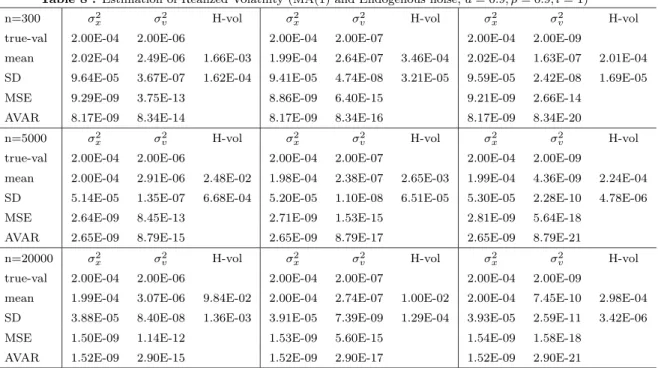
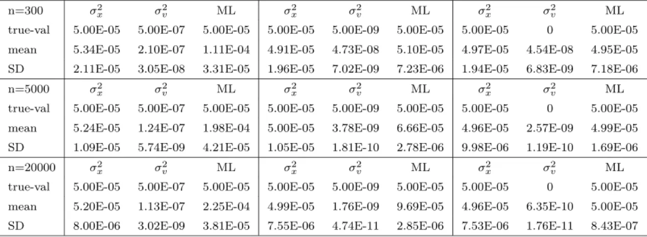
Among many Monte-Carlo simulations, we summarize our main results as Tables of Appendix C. If we knew the fact that the underlying noise process is MA(q) and its distribution is Gaussian, we can use the maximum likelihood (ML) estimation for the model that the observations are the sum of the signal process and the market
noise process. By using the standard arguments of statistical asymptotic theory for parametric models, the ML estimation is asymptotically efficient. We have confirmed this fact in Table 11 when the noise process is MA(0). When the noise process is MA(1), however, the ML estimator has lose the asymptotic efficiency while the SIML estimator gives reasonable and stable estimates.
For the standard case of MA(0) and the MA(1) case for noise terms we give the results of the SIML estimation as Tables 1-3. (We note that a stands for the MA(1) coefficient.) The finite sample efficiency of the ML estimator lose its power rather quickly while the SIML estimator has robustness against this type of autocorrela-tions. (Table 11 shows some results of the ML estimation when we knew that the true process is MA(1).) For the case of the endogenous noise we give Tables 4-6 with
and without autocorrelated noise terms. In these tables l = 0 stands for the cases
of instantaneous endogeneity while l = 1 stands for the cases when there are some
lagged effects between the signal and noise terms. We also have conducted some
extreme experiments such as the cases when a = 0.95 and AR(1) with b = 0.95.
They are summarized in Tables 7-10.
By examining the results of our simulations we can conclude that we can estimate both the realized volatility of the hidden martingale part and the market noise part reasonably in all cases we have examined by the SIML estimation. We also have conducted a number of further simulations and the some details have been given in Kunitomo and Sato (2008b).
5. Conclusions
In this paper, we have shown that the Separating Information Maximum Like-lihood (SIML) estimator has the asymptotic robustness in the sense that it is con-sistent and it has the asymptotic normality under a fairly general conditions even when the standard conditions are not satisfied. They include the cases when the micro-market noises are possibly autocorrelated and they are endogenously corre-lated with the underlying continuous signal processes. By conducting large number of simulations, we have confirmed that the SIML estimator has reasonable robust
properties in finite samples even in these non-standard situations.
As a concluding remark, the SIML estimator is very simple and it can be prac-tically used not only for the realized volatility but also the realized covariance of the multivariate high frequency financial series. Some applications on the analysis of financial futures markets have been reported in Kunitomo and Sato (2008b) for example.
References
[1] Barndorff-Nielsen, O., P. Hansen, A. Lunde and N. Shephard (2008), “Design-ing realized kernels to measure the ex-post variation of equity prices in the presence of noise, Econometrica, Vol.76-6, 1481-1536.
[2] Hall, P. and C. Heyde (1980), Martingale Limit Theory and its Applications,
Academic Press.
[3] Kunitomo, N. and S. Sato (2008a), “Separating Information Maximum Like-lihood Estimation of Realized Volatility and Covariance with Micro-Market Noise,” Discussion Paper CIRJE-F-581, Graduate School of Economics, Uni-versity of Tokyo, (http://www.e.u-tokyo.ac.jp/cirje/research/dp/2008).
[4] Kunitomo, N. and S. Sato (2008b), “Realized Volatility, Covariance and Hedg-ing Coefficient of Nikkei-225 Futures with Micro-Market Noise,” Discussion Paper CIRJE-F-601, Graduate School of Economics, University of Tokyo, (http://www.e.u-tokyo.ac.jp/cirje/research/dp/2008).
[5] Kunitomo, N. and S. Sato (2009), “The SIML Estimation of the Realized Volatility and Hedging Coefficient of Nikkei-225 Futures with Micro-Market
Noise,” submitted to Mathematics and Computers in Simulations,
Appendices
We gather some details in Appendices. In Appendix A we give the mathematical derivation of Theorem 1 and discussion of Theorem 1 of Kunitomo and Sato (2008a). Then in Appendix B we give some formulas used in Appendix A and Section 2. (The derivations are similar to the ones in Kunitomo and Sato (2008a) and they are omitted.) In Appendix C we give some tables.
(I) APPENDIX A : On Derivations of Theorem 1 and Theorem 1 of Kunitomo-Sato (2008a)
From Section 6 of Kunitomo and Sato (2009a), we shall investigate the asymptotic distribution of √ m ⎡ ⎣n i,j=1 cijrirj−δij ti ti−1σ 2 x(s)ds ⎤ ⎦ (A.1) = 2√m i>j cijrirj+ √ m n i=1 ciir2i − ti ti−1σ 2 x(s)ds , where δij = 1 (i=j);δij = 0 (i=j).
The second term is equivalent to
√ m n i=1 ri2− ti ti−1σ 2 x(s)ds+ (cii−1)ri2 (A.2) = m n √ n n i=1 r2 i − ti ti−1σ 2 x(s)ds +√m n i=1 (cii−1)(ri2− ti ti−1σ 2 x(s)ds) +√m n i=1 (cii−1) ti ti−1 σ 2 x(s)ds .
We notice that Jacod-Protter (1998 Annals of Probability) have shown that
√ n n i=1 r2 i − ti ti−1σ 2 x(s)ds =Op(1).
By using the fact thatcii−1 (i= 1,· · ·, n) are bounded, we find that as √m/n→0
the second term of (A.2) is asymptotically equivalent to
√ m n i=1 (cii−1) ti ti−1σ 2 x(s)ds = n i=1 1 2√m sin[2πm 2n+1(2i−1)] sin[2n2π+1(2i−1)] ti ti−1σ 2 x(s)ds . (A.3)
When σs =σ (constant), √ m n i=1 (cii−1) ti ti−1σ 2 x(s)ds = σ2 √ m n n i=1 (cii−1) = σ2 √ m n n+ 1 2−n →0
as √m/n → 0. There are some cases that (A.3) is o(1) because ti
ti−1σ 2
sds ≤
(1/n) sup0≤s≤1σ2
s. Generally, this term may be small because it is bounded and
|n i=1 (cii−1) ti ti−1σ 2 x(s)ds|2 = n i=1 (cii−1)2 n i=1 ( ti ti−1σ 2 x(s)ds)2 ≤ 1 n n i=1 (cii−1)2 sup 0≤s≤tσ 2 x(s) 2 =O(1 m).
However, we have not proven that it is o(1) under the general situations. The
asymptotic variance of the first term of (A.2) is
4 i<j mc2ijE[r2i]E[rj2] = 2 n i,j=1 mc2ijE[ri2]E[rj2]−2 n i=1 mc2ii(E[r2i])2 = 2 n i,j=1 E[ri2]E[r2j] + 2 n i,j=1 (mc2ij −1)E[ri2]E[rj2]−2 n i=1 mc2ii(E[ri2])2 .
For the third term, we have
n i=1 mc2ii(E[r2i])2 ≤ sup 0≤≤1σ 2 x(s) 2 m n2 n i=1 c2ii→0
as m/n→0. Then the asymptotic variance of (2.14) becomes
Vn (A.4) = 2 n i=1 ti ti−1σ 2 x(s)ds 2 + 2 n i,j=1 (mc2ij −1) ti ti−1σ 2 x(s)ds tj tj−1σ 2 x(s)ds → 2 1 0 σ 2 x(s)ds 2 + 2 lim n→∞ n i,j=1 (mc2ij −1) ti ti−1σ 2 x(s)ds tj tj−1σ 2 x(s)ds =V .
The second term is bounded because 1 n2 n i,j=1 |mc2ij −1| ≤1 + m n2 n i,j=1 c2ij
and it is likely to be small, but we have not proven that it iso(1). Hence presently the statement of Theorem 1 of Kunitomo and Sato (2008a) should be slightly modified as √ m ˆ σ2 x−σ2x− n i=1 (cii−1) ti ti−1σ 2 x(s)ds w →N [0, V] . (A.5)
When the volatility function is constant (σx(s) =σ),
ti ti−1σ 2 x(s)ds =σ2 1 n ,
the second term vanishes because 1 n2 n i,j=1 (mc2ij −1) = 1 n2 n2+n+ 1 4−n 2→0 and then V = 2 1 0 σ 2 x(s)ds 2 . (A.6)
There are some other cases that second term ofVn is o(1) because we have (A.4).
(II) APPENDIX B : Some Formulas
In our derivations we have used elementary relations of trigonometric functions and their sums. From (2.16), we have
n j=1 cjj =n+ 1 2 . (B.7) From (2.15), we rewrite c2ij = ( 2 m) 2 m k,k=1 siksjksiksjk = (1 m) 2 m k,k=1 cos[ 2π 2n+ 1(i+j−1)(k− 1 2)] + cos[ 2π 2n+ 1(i−j)(k− 1 2)] ×cos[ 2π 2n+ 1(i+j−1(k − 1 2)] + cos[ 2π 2n+ 1(i−j)(k −1 2)] = (1 m) 2 m k,k=1 1 2cos[ 2π 2n+ 1(i+j−1)(k+k −1) + 1 2cos[ 2π 2n+ 1(i+j−1)(k−k ) +2 1 2cos[ 2π 2n+ 1((i+j −1)(k− 1 2) + (k − 1 2)(i−j))]
+1 2cos[ 2π 2n+ 1((i+j−1)(k− 1 2)−(k − 1 2)(i−j))] +1 2cos[ 2π 2n+ 1(i−j)(k+k −1) + 1 2cos[ 2π 2n+ 1(i−j)(k−k ) . and hence c2jj = 1 + 2 m m k=1 cos[ 2π 2n+ 1(k− 1 2)(2j−1)] + 1 2m2 m k,k=1 cos[ 2π 2n+ 1(2j−1)(k+k −1)] + cos[ 2π 2n+ 1(2j−1)(k−k )] .
By using the relation nj=1cos[2n2π+1(2k−1)(2j−1)] = 12 for k ≥ 1 and after some calculations, it is straightforward to show
1 n n i=1 (c2 ii−1)→0, (B.8) 1 n n i=1 (cii−1)2 →0, (B.9) and m n i,j=1 c2ij = (n+ 1 2) 2 (B.10)
by using the relation n
j=1sjksjk =δkk(n2 +14).
(III) APPENDIX C : TABLES
In Tables 1-11 σ2
x and σv2 are the true parameter variances and we give their
corre-sponding estimates when we have the constant volatility model. Mean and SD in Tables are the sample mean and the standard deviation of the SIML estimator (or the ML estimator) in simulations. H-vol stands for the historical volatility.
Table 1 : Estimation of Realized Volatility (standard case,vt∼i.i.d.Normal)
n=300 σ2x σ2v H-vol σ2x σv2 H-vol σx2 σv2 H-vol true-val 2.00E-04 2.00E-06 2.00E-04 2.00E-07 2.00E-04 2.00E-09
mean 2.05E-04 2.18E-06 1.40E-03 2.00E-04 3.82E-07 3.19E-04 2.01E-04 1.84E-07 2.01E-04 SD 9.61E-05 3.22E-07 1.35E-04 9.16E-05 5.61E-08 2.67E-05 9.29E-05 2.69E-08 1.61E-05 MSE 9.27E-09 1.36E-13 8.40E-09 3.61E-14 8.63E-09 3.39E-14
AVAR 8.17E-09 8.34E-14 8.17E-09 8.34E-16 8.17E-09 8.34E-20
n=5000 σ2x σ2v H-vol σ2x σv2 H-vol σx2 σv2 H-vol true-val 2.00E-04 2.00E-06 2.00E-04 2.00E-07 2.00E-04 2.00E-09
mean 2.07E-04 2.01E-06 2.02E-02 2.01E-04 2.10E-07 2.20E-03 2.00E-04 1.23E-08 2.20E-04 SD 5.37E-05 9.44E-08 4.93E-04 5.12E-05 9.68E-09 5.22E-05 5.27E-05 5.68E-10 4.35E-06 MSE 2.92E-09 8.99E-15 2.62E-09 2.03E-16 2.78E-09 1.06E-16
AVAR 2.65E-09 8.79E-15 2.65E-09 8.79E-17 2.65E-09 8.79E-21
n=20000 σ2x σ2v H-vol σ2x σv2 H-vol σx2 σv2 H-vol
true-val 2.00E-04 2.00E-06 2.00E-04 2.00E-07 2.00E-04 2.00E-09
mean 2.05E-04 2.00E-06 8.02E-02 2.00E-04 2.03E-07 8.20E-03 2.00E-04 4.54E-09 2.80E-04 SD 4.10E-05 5.47E-08 9.82E-04 3.98E-05 5.43E-09 9.91E-05 3.90E-05 1.19E-10 2.87E-06 MSE 1.70E-09 3.00E-15 1.59E-09 3.59E-17 1.52E-09 6.46E-18
AVAR 1.52E-09 2.90E-15 1.52E-09 2.90E-17 1.52E-09 2.90E-21
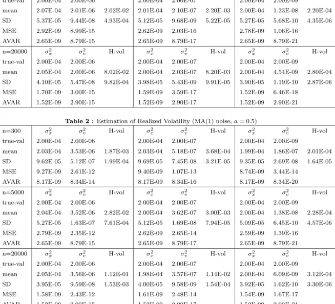
Table 2 : Estimation of Realized Volatility (MA(1) noise,a= 0.5)
n=300 σ2x σ2v H-vol σ2x σv2 H-vol σx2 σv2 H-vol
true-val 2.00E-04 2.00E-06 2.00E-04 2.00E-07 2.00E-04 2.00E-09
mean 2.03E-04 3.53E-06 1.87E-03 2.03E-04 5.18E-07 3.68E-04 1.99E-04 1.86E-07 2.01E-04 SD 9.62E-05 5.12E-07 1.99E-04 9.69E-05 7.45E-08 3.21E-05 9.35E-05 2.69E-08 1.64E-05 MSE 9.27E-09 2.61E-12 9.40E-09 1.07E-13 8.74E-09 3.44E-14
AVAR 8.17E-09 8.34E-14 8.17E-09 8.34E-16 8.17E-09 8.34E-20
n=5000 σ2x σ2v H-vol σ2x σv2 H-vol σx2 σv2 H-vol
true-val 2.00E-04 2.00E-06 2.00E-04 2.00E-07 2.00E-04 2.00E-09
mean 2.04E-04 3.52E-06 2.82E-02 2.00E-04 3.62E-07 3.00E-03 2.00E-04 1.38E-08 2.28E-04 SD 5.27E-05 1.63E-07 7.61E-04 5.12E-05 1.69E-08 7.94E-05 5.09E-05 6.45E-10 4.57E-06 MSE 2.79E-09 2.35E-12 2.62E-09 2.65E-14 2.59E-09 1.39E-16
AVAR 2.65E-09 8.79E-15 2.65E-09 8.79E-17 2.65E-09 8.79E-21
n=20000 σ2x σ2v H-vol σ2x σv2 H-vol σx2 σv2 H-vol true-val 2.00E-04 2.00E-06 2.00E-04 2.00E-07 2.00E-04 2.00E-09
mean 2.05E-04 3.56E-06 1.12E-01 1.98E-04 3.57E-07 1.14E-02 2.00E-04 6.09E-09 3.12E-04 SD 3.95E-05 9.59E-08 1.53E-03 4.00E-05 9.58E-09 1.54E-04 3.92E-05 1.62E-10 3.30E-06 MSE 1.58E-09 2.43E-12 1.61E-09 2.48E-14 1.54E-09 1.67E-17
AVAR 1.52E-09 2.90E-15 1.52E-09 2.90E-17 1.52E-09 2.90E-21
Data generating process:
yt=xt+σv2/(1 +a2)vt xt=xt−1+σ2x/nut
vt=wt−awt−1
Table 3 :Estimation of Realized Volatility (MA(1) noise,a=−0.5)
n=300 σ2x σ2v H-vol σ2x σv2 H-vol σx2 σv2 H-vol true-val 2.00E-04 2.00E-06 2.00E-04 2.00E-07 2.00E-04 2.00E-09
mean 2.07E-04 8.40E-07 9.17E-04 2.02E-04 2.47E-07 2.71E-04 2.02E-04 1.82E-07 2.00E-04 SD 9.59E-05 1.25E-07 8.22E-05 9.65E-05 3.65E-08 2.26E-05 9.40E-05 2.66E-08 1.57E-05 MSE 9.24E-09 1.36E-12 9.32E-09 3.53E-15 8.83E-09 3.33E-14
AVAR 8.17E-09 8.34E-14 8.17E-09 8.34E-16 8.17E-09 8.34E-20
n=5000 σ2x σ2v H-vol σ2x σv2 H-vol σx2 σv2 H-vol true-val 2.00E-04 2.00E-06 2.00E-04 2.00E-07 2.00E-04 2.00E-09
mean 2.05E-04 4.96E-07 1.22E-02 2.02E-04 5.89E-08 1.40E-03 2.00E-04 1.08E-08 2.12E-04 SD 5.21E-05 2.34E-08 2.75E-04 5.30E-05 2.81E-09 3.10E-05 5.29E-05 4.88E-10 4.35E-06 MSE 2.75E-09 2.26E-12 2.81E-09 1.99E-14 2.79E-09 7.71E-17
AVAR 2.65E-09 8.79E-15 2.65E-09 8.79E-17 2.65E-09 8.79E-21
n=20000 σ2x σ2v H-vol σ2x σv2 H-vol σx2 σv2 H-vol
true-val 2.00E-04 2.00E-06 2.00E-04 2.00E-07 2.00E-04 2.00E-09
mean 2.06E-04 4.52E-07 4.82E-02 2.01E-04 4.75E-08 5.00E-03 2.01E-04 2.99E-09 2.48E-04 SD 4.01E-05 1.23E-08 5.47E-04 3.84E-05 1.26E-09 5.58E-05 4.01E-05 8.07E-11 2.45E-06 MSE 1.64E-09 2.40E-12 1.48E-09 2.33E-14 1.61E-09 9.88E-19
AVAR 1.52E-09 2.90E-15 1.52E-09 2.90E-17 1.52E-09 2.90E-21
Data generating process: same as Table 2.
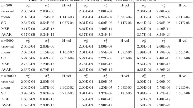
Table 4 : Estimation of Realized Volatility (Endogenous noise,ρ= 0.5, l= 0)
n=300 σ2x σ2v H-vol σ2x σv2 H-vol σx2 σv2 H-vol true-val 2.00E-04 2.00E-06 2.00E-04 2.00E-07 2.00E-04 2.00E-09
mean 2.02E-04 1.76E-06 1.14E-03 1.98E-04 4.64E-07 3.68E-04 1.97E-04 2.02E-07 2.11E-04 SD 9.54E-05 2.54E-07 1.07E-04 9.31E-05 6.62E-08 3.14E-05 9.44E-05 2.98E-08 1.71E-05 MSE 9.11E-09 1.23E-13 8.67E-09 7.40E-14 8.93E-09 4.10E-14
AVAR 8.17E-09 8.34E-14 8.17E-09 8.34E-16 8.17E-09 8.34E-20
n=5000 σ2x σ2v H-vol σ2x σv2 H-vol σx2 σv2 H-vol
true-val 2.00E-04 2.00E-06 2.00E-04 2.00E-07 2.00E-04 2.00E-09
mean 2.02E-04 1.15E-06 1.16E-02 2.01E-04 1.55E-07 1.65E-03 1.99E-04 1.58E-08 2.55E-04 SD 5.27E-05 5.42E-08 2.82E-04 5.27E-05 7.22E-09 3.77E-05 5.13E-05 7.48E-10 5.19E-06 MSE 2.78E-09 7.20E-13 2.78E-09 2.08E-15 2.64E-09 1.90E-16
AVAR 2.65E-09 8.79E-15 2.65E-09 8.79E-17 2.65E-09 8.79E-21
n=20000 σ2x σ2v H-vol σ2x σv2 H-vol σx2 σv2 H-vol
true-val 2.00E-04 2.00E-06 2.00E-04 2.00E-07 2.00E-04 2.00E-09
mean 2.03E-04 1.07E-06 4.30E-02 2.00E-04 1.25E-07 5.09E-03 2.00E-04 5.78E-09 3.29E-04 SD 3.99E-05 2.87E-08 5.21E-04 3.91E-05 3.37E-09 6.12E-05 3.96E-05 1.57E-10 3.50E-06 MSE 1.60E-09 8.60E-13 1.53E-09 5.66E-15 1.57E-09 1.43E-17
AVAR 1.52E-09 2.90E-15 1.52E-09 2.90E-17 1.52E-09 2.90E-21
Data generating process:
yt=xt+σ2vvt xt=xt−1+ σ2x/nut vt= (1−ρ)wt+ρut−l ut∼i.i.d.N(0,1), wt∼i.i.d.N(0,1)
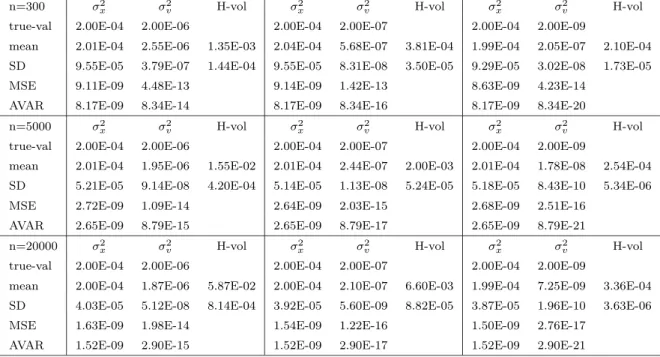
Table 5 :Estimation of Realized Volatility (MA(1) and Endogenous noise,a= 0.5, ρ= 0.5, l= 0)
n=300 σ2x σ2v H-vol σ2x σv2 H-vol σx2 σv2 H-vol true-val 2.00E-04 2.00E-06 2.00E-04 2.00E-07 2.00E-04 2.00E-09
mean 2.01E-04 2.55E-06 1.35E-03 2.04E-04 5.68E-07 3.81E-04 1.99E-04 2.05E-07 2.10E-04 SD 9.55E-05 3.79E-07 1.44E-04 9.55E-05 8.31E-08 3.50E-05 9.29E-05 3.02E-08 1.73E-05 MSE 9.11E-09 4.48E-13 9.14E-09 1.42E-13 8.63E-09 4.23E-14
AVAR 8.17E-09 8.34E-14 8.17E-09 8.34E-16 8.17E-09 8.34E-20
n=5000 σ2x σ2v H-vol σ2x σv2 H-vol σx2 σv2 H-vol true-val 2.00E-04 2.00E-06 2.00E-04 2.00E-07 2.00E-04 2.00E-09
mean 2.01E-04 1.95E-06 1.55E-02 2.01E-04 2.44E-07 2.00E-03 2.01E-04 1.78E-08 2.54E-04 SD 5.21E-05 9.14E-08 4.20E-04 5.14E-05 1.13E-08 5.24E-05 5.18E-05 8.43E-10 5.34E-06 MSE 2.72E-09 1.09E-14 2.64E-09 2.03E-15 2.68E-09 2.51E-16
AVAR 2.65E-09 8.79E-15 2.65E-09 8.79E-17 2.65E-09 8.79E-21
n=20000 σ2x σ2v H-vol σ2x σv2 H-vol σx2 σv2 H-vol
true-val 2.00E-04 2.00E-06 2.00E-04 2.00E-07 2.00E-04 2.00E-09
mean 2.00E-04 1.87E-06 5.87E-02 2.00E-04 2.10E-07 6.60E-03 1.99E-04 7.25E-09 3.36E-04 SD 4.03E-05 5.12E-08 8.14E-04 3.92E-05 5.60E-09 8.82E-05 3.87E-05 1.96E-10 3.63E-06 MSE 1.63E-09 1.98E-14 1.54E-09 1.22E-16 1.50E-09 2.76E-17
AVAR 1.52E-09 2.90E-15 1.52E-09 2.90E-17 1.52E-09 2.90E-21
Data generating process:
yt=xt+σv2/(1 +a2)vt xt=xt−1+ σ2x/nut vt=t−at−1 t= (1−ρ)wt+ρut−l ut∼i.i.d.N(0,1), wt∼i.i.d.N(0,1)
Table 6 :Estimation of Realized Volatility (MA(1) and Endogenous noise,a= 0.8, ρ= 0.9, l= 1)
n=300 σ2x σ2v H-vol σ2x σv2 H-vol σx2 σv2 H-vol true-val 2.00E-04 2.00E-06 2.00E-04 2.00E-07 2.00E-04 2.00E-09
mean 1.98E-04 1.71E-06 7.86E-04 2.00E-04 1.88E-08 6.91E-05 2.01E-04 1.39E-07 1.74E-04 SD 9.23E-05 2.47E-07 9.13E-05 9.30E-05 2.94E-09 7.78E-06 9.42E-05 2.02E-08 1.39E-05 MSE 8.53E-09 1.43E-13 8.65E-09 3.28E-14 8.88E-09 1.92E-14
AVAR 8.17E-09 8.34E-14 8.17E-09 8.34E-16 8.17E-09 8.34E-20
n=5000 σ2x σ2v H-vol σ2x σv2 H-vol σx2 σv2 H-vol true-val 2.00E-04 2.00E-06 2.00E-04 2.00E-07 2.00E-04 2.00E-09
mean 2.00E-04 2.81E-06 2.10E-02 2.01E-04 2.13E-07 1.51E-03 2.00E-04 2.12E-09 1.11E-04 SD 5.31E-05 1.33E-07 6.02E-04 5.16E-05 1.02E-08 4.47E-05 5.15E-05 1.02E-10 2.51E-06 MSE 2.82E-09 6.67E-13 2.66E-09 2.61E-16 2.65E-09 2.51E-20
AVAR 2.65E-09 8.79E-15 2.65E-09 8.79E-17 2.65E-09 8.79E-21
n=20000 σ2x σ2v H-vol σ2x σv2 H-vol σx2 σv2 H-vol
true-val 2.00E-04 2.00E-06 2.00E-04 2.00E-07 2.00E-04 2.00E-09
mean 2.01E-04 3.01E-06 9.06E-02 2.01E-04 2.65E-07 7.70E-03 2.00E-04 7.30E-11 7.13E-05 SD 4.01E-05 8.08E-08 1.28E-03 4.05E-05 6.97E-09 1.08E-04 3.96E-05 1.96E-12 9.98E-07 MSE 1.61E-09 1.04E-12 1.64E-09 4.28E-15 1.56E-09 3.71E-18
AVAR 1.52E-09 2.90E-15 1.52E-09 2.90E-17 1.52E-09 2.90E-21
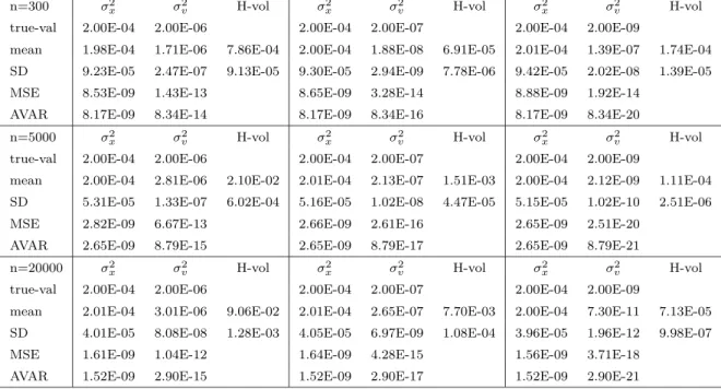
Table 7 : Estimation of Realized Volatility (MA(1) noise,a= 0.95)
n=300 σ2x σ2v H-vol σ2x σv2 H-vol σx2 σv2 H-vol true-val 2.00E-04 2.00E-06 2.00E-04 2.00E-07 2.00E-04 2.00E-09
mean 1.99E-04 1.71E-06 7.86E-04 1.99E-04 1.90E-08 6.89E-05 2.02E-04 1.39E-07 1.74E-04 SD 9.40E-05 2.53E-07 9.35E-05 9.22E-05 2.96E-09 7.87E-06 9.67E-05 2.05E-08 1.44E-05 MSE 8.83E-09 1.49E-13 8.51E-09 3.28E-14 9.35E-09 1.91E-14
AVAR 8.17E-09 8.34E-14 8.17E-09 8.34E-16 8.17E-09 8.34E-20
n=5000 σ2x σ2v H-vol σ2x σv2 H-vol σx2 σv2 H-vol true-val 2.00E-04 2.00E-06 2.00E-04 2.00E-07 2.00E-04 2.00E-09
mean 2.02E-04 2.81E-06 2.10E-02 1.99E-04 2.12E-07 1.51E-03 1.99E-04 2.12E-09 1.11E-04 SD 5.25E-05 1.30E-07 5.94E-04 5.17E-05 9.97E-09 4.37E-05 5.08E-05 9.98E-11 2.45E-06 MSE 2.76E-09 6.71E-13 2.67E-09 2.52E-16 2.58E-09 2.50E-20
AVAR 2.65E-09 8.79E-15 2.65E-09 8.79E-17 2.65E-09 8.79E-21
n=20000 σ2x σ2v H-vol σ2x σv2 H-vol σx2 σv2 H-vol
true-val 2.00E-04 2.00E-06 2.00E-04 2.00E-07 2.00E-04 2.00E-09
mean 2.03E-04 3.02E-06 9.07E-02 1.99E-04 2.65E-07 7.69E-03 2.01E-04 7.30E-11 7.13E-05 SD 3.99E-05 8.17E-08 1.26E-03 3.90E-05 7.18E-09 1.10E-04 3.95E-05 1.98E-12 1.01E-06 MSE 1.60E-09 1.04E-12 1.52E-09 4.27E-15 1.56E-09 3.71E-18
AVAR 1.52E-09 2.90E-15 1.52E-09 2.90E-17 1.52E-09 2.90E-21
Data generating process: same as Table 2.
Table 8 :Estimation of Realized Volatility (MA(1) and Endogenous noise,a= 0.9, ρ= 0.9, l= 1)
n=300 σ2x σ2v H-vol σ2x σv2 H-vol σx2 σv2 H-vol true-val 2.00E-04 2.00E-06 2.00E-04 2.00E-07 2.00E-04 2.00E-09
mean 2.02E-04 2.49E-06 1.66E-03 1.99E-04 2.64E-07 3.46E-04 2.02E-04 1.63E-07 2.01E-04 SD 9.64E-05 3.67E-07 1.62E-04 9.41E-05 4.74E-08 3.21E-05 9.59E-05 2.42E-08 1.69E-05 MSE 9.29E-09 3.75E-13 8.86E-09 6.40E-15 9.21E-09 2.66E-14
AVAR 8.17E-09 8.34E-14 8.17E-09 8.34E-16 8.17E-09 8.34E-20
n=5000 σ2x σ2v H-vol σ2x σv2 H-vol σx2 σv2 H-vol
true-val 2.00E-04 2.00E-06 2.00E-04 2.00E-07 2.00E-04 2.00E-09
mean 2.00E-04 2.91E-06 2.48E-02 1.98E-04 2.38E-07 2.65E-03 1.99E-04 4.36E-09 2.24E-04 SD 5.14E-05 1.35E-07 6.68E-04 5.20E-05 1.10E-08 6.51E-05 5.30E-05 2.28E-10 4.78E-06 MSE 2.64E-09 8.45E-13 2.71E-09 1.53E-15 2.81E-09 5.64E-18
AVAR 2.65E-09 8.79E-15 2.65E-09 8.79E-17 2.65E-09 8.79E-21
n=20000 σ2x σ2v H-vol σ2x σv2 H-vol σx2 σv2 H-vol
true-val 2.00E-04 2.00E-06 2.00E-04 2.00E-07 2.00E-04 2.00E-09
mean 1.99E-04 3.07E-06 9.84E-02 2.00E-04 2.74E-07 1.00E-02 2.00E-04 7.45E-10 2.98E-04 SD 3.88E-05 8.40E-08 1.36E-03 3.91E-05 7.39E-09 1.29E-04 3.93E-05 2.59E-11 3.42E-06 MSE 1.50E-09 1.14E-12 1.53E-09 5.60E-15 1.54E-09 1.58E-18
AVAR 1.52E-09 2.90E-15 1.52E-09 2.90E-17 1.52E-09 2.90E-21
Table 9 : Estimation of Realized Volatility (AR(1) noise,b= 0.95)
n=300 σ2x σ2v H-vol σ2x σv2 H-vol σx2 σv2 H-vol true-val 2.00E-04 2.00E-06 2.00E-04 2.00E-07 2.00E-04 2.00E-09
mean 2.24E-04 2.39E-07 2.59E-04 2.04E-04 1.89E-07 2.06E-04 2.00E-04 1.82E-07 1.99E-04 SD 1.05E-04 3.43E-08 2.11E-05 9.72E-05 2.80E-08 1.72E-05 9.65E-05 2.63E-08 1.63E-05 MSE 1.17E-08 3.10E-12 9.47E-09 9.17E-16 9.31E-09 3.29E-14
AVAR 8.17E-09 8.34E-14 8.17E-09 8.34E-16 8.17E-09 8.34E-20
n=5000 σ2x σ2v H-vol σ2x σv2 H-vol σx2 σv2 H-vol true-val 2.00E-04 2.00E-06 2.00E-04 2.00E-07 2.00E-04 2.00E-09
mean 2.43E-04 6.31E-08 1.20E-03 2.04E-04 1.56E-08 3.00E-04 1.99E-04 1.03E-08 2.01E-04 SD 6.34E-05 2.89E-09 2.39E-05 5.22E-05 7.30E-10 6.00E-06 5.12E-05 4.91E-10 4.10E-06 MSE 5.89E-09 3.75E-12 2.74E-09 3.40E-14 2.62E-09 6.96E-17
AVAR 2.65E-09 8.79E-15 2.65E-09 8.79E-17 2.65E-09 8.79E-21
n=20000 σ2x σ2v H-vol σ2x σv2 H-vol σx2 σv2 H-vol
true-val 2.00E-04 2.00E-06 2.00E-04 2.00E-07 2.00E-04 2.00E-09
mean 2.35E-04 5.46E-08 4.20E-03 2.04E-04 7.75E-09 6.00E-04 2.01E-04 2.59E-09 2.04E-04 SD 4.62E-05 1.44E-09 4.22E-05 4.08E-05 2.10E-10 6.05E-06 3.97E-05 6.97E-11 2.03E-06 MSE 3.35E-09 3.78E-12 1.68E-09 3.70E-14 1.58E-09 3.56E-19
AVAR 1.52E-09 2.90E-15 1.52E-09 2.90E-17 1.52E-09 2.90E-21
Data generating process:
yt=xt+σ2v(1−a2)vt xt=xt−1+ σ2x/nut vt=bvt−1+wt ut∼i.i.d.N(0,1), wt∼i.i.d.N(0,1)
Table 10 : Estimation of Realized Volatility (MA(1) and Endogenous noise,a= 0.9, ρ= 0.9, l= 0) n=300 σ2x σ2v H-vol σ2x σv2 H-vol σx2 σv2 H-vol
true-val 2.00E-04 2.00E-06 2.00E-04 2.00E-07 2.00E-04 2.00E-09
mean 2.01E-04 4.46E-06 2.14E-03 2.00E-04 8.75E-07 4.91E-04 1.99E-04 2.24E-07 2.15E-04 SD 9.44E-05 6.43E-07 2.43E-04 9.61E-05 1.28E-07 4.94E-05 9.48E-05 3.31E-08 1.76E-05 MSE 8.90E-09 6.48E-12 9.24E-09 4.72E-13 8.99E-09 5.03E-14
AVAR 8.17E-09 8.34E-14 8.17E-09 8.34E-16 8.17E-09 8.34E-20
n=5000 σ2x σ2v H-vol σ2x σv2 H-vol σx2 σv2 H-vol true-val 2.00E-04 2.00E-06 2.00E-04 2.00E-07 2.00E-04 2.00E-09
mean 2.00E-04 3.53E-06 2.66E-02 2.00E-04 4.37E-07 3.26E-03 1.99E-04 2.43E-08 2.84E-04 SD 5.20E-05 1.67E-07 7.58E-04 5.28E-05 2.08E-08 9.32E-05 5.01E-05 1.15E-09 6.17E-06 MSE 2.70E-09 2.38E-12 2.79E-09 5.65E-14 2.51E-09 4.98E-16
AVAR 2.65E-09 8.79E-15 2.65E-09 8.79E-17 2.65E-09 8.79E-21
n=20000 σ2x σ2v H-vol σ2x σv2 H-vol σx2 σv2 H-vol true-val 2.00E-04 2.00E-06 2.00E-04 2.00E-07 2.00E-04 2.00E-09
mean 2.00E-04 3.40E-06 1.02E-01 2.01E-04 3.80E-07 1.12E-02 1.99E-04 1.13E-08 4.18E-04 SD 3.92E-05 9.07E-08 1.44E-03 3.91E-05 1.03E-08 1.59E-04 3.85E-05 3.03E-10 4.93E-06 MSE 1.54E-09 1.96E-12 1.53E-09 3.25E-14 1.49E-09 8.62E-17
AVAR 1.52E-09 2.90E-15 1.52E-09 2.90E-17 1.52E-09 2.90E-21
Table 11 : Comparing with ML (MA(1) noise,a= 0.5, α= 0.45)
n=300 σ2x σ2v ML σ2x σv2 ML σx2 σv2 ML true-val 5.00E-05 5.00E-07 5.00E-05 5.00E-05 5.00E-09 5.00E-05 5.00E-05 0 5.00E-05 mean 5.34E-05 2.10E-07 1.11E-04 4.91E-05 4.73E-08 5.10E-05 4.97E-05 4.54E-08 4.95E-05 SD 2.11E-05 3.05E-08 3.31E-05 1.96E-05 7.02E-09 7.23E-06 1.94E-05 6.83E-09 7.18E-06 n=5000 σ2x σ2v ML σ2x σv2 ML σx2 σv2 ML true-val 5.00E-05 5.00E-07 5.00E-05 5.00E-05 5.00E-09 5.00E-05 5.00E-05 0 5.00E-05 mean 5.24E-05 1.24E-07 1.98E-04 5.00E-05 3.78E-09 6.66E-05 4.96E-05 2.57E-09 4.99E-05 SD 1.09E-05 5.74E-09 4.21E-05 1.05E-05 1.81E-10 2.78E-06 9.98E-06 1.19E-10 1.69E-06 n=20000 σ2x σ2v ML σ2x σv2 ML σx2 σv2 ML true-val 5.00E-05 5.00E-07 5.00E-05 5.00E-05 5.00E-09 5.00E-05 5.00E-05 0 5.00E-05 mean 5.20E-05 1.13E-07 2.25E-04 4.99E-05 1.76E-09 9.69E-05 4.96E-05 6.35E-10 5.00E-05 SD 8.00E-06 3.02E-09 3.81E-05 7.55E-06 4.74E-11 2.85E-06 7.53E-06 1.76E-11 8.43E-07