DOI:10.3233/JIFS-169280 IOS Press
An improved clustering routing mechanism
for wireless Ad hoc network
Tong Wang
a, Yunfeng Wang
aand Chong Han
b,∗aCollege of Information and Communication Engineering, Harbin Engineering University, China bInstitute for Communication Systems (ICS), 5GIC, University of Surrey, Guildford, UK
Abstract. In Wireless Ad hoc Networks (WANET), to organize sensor nodes for data collection is an important research issue. Clustering is an effective technique for prolonging the network lifetime. However, the Cluster Header (CH) in a cluster always involves a lot of data forwarding tasks, rather than its Cluster Members (CMs). This energy consumption overloading inevitably leads to the “hot spot” problem. With these in mind, an Energy-Balanced and Unequally-Layered Routing Protocol (EBULRP) is proposed in this article. The main emphasis is on balancing the energy consumption among CHs. In our design, the network is decoupled into multiple layers with different width, where the radius of clusters is differentiated at each layer. The core is to organize those CHs closer to the sink node, with more energy for inter-cluster data forwarding. Simulation results show that the proposed EBULRP effectively balances the energy consumption among CHs, and further prolongs the network lifetime.
Keywords: Wireless sensor networks, communication protocol, routing, energy efficiency 1. Introduction
Wireless Ad hoc Network (WANET) is a decentral-ized type of wireless network. Over the last decade, the research on Wireless Sensor Networks (WSNs) or WANETs has been receiving great attention from academic and industrial communities. WSNs gener-ally include a number of sensor nodes and given sink node deployed in an area, mainly for event monitor-ing and detection, data collection and transmission [1–4]. However, sensor nodes are inherently battery-powered, and it is also difficult to recharge their energy once being used. In light of this, how to pro-long the network lifetime by efficiently utilizing the limited energy of sensor nodes is a primary objective for protocol design in WSNs [5–8].
In literature, the energy consumption module in WSNs generally includes sensing module, process-ing module, and wireless communication module. ∗Corresponding author. Chong Han, Institute for
Communi-cation Systems (ICS), 5GIC, University of Surrey, Guildford, UK. Tel.: +44 1483682519; Fax: +44 1483689551; E-mail: chong.han@surrey.ac.uk.
Among them, the wireless communication module concerning data transmission consumes most of the energy. Compared with flat routing schemes [9–11], those schemes based on clustering [12–15] can effec-tively improve the network scalability. While in clustering routing, sensor nodes are generally divided into two parts, which are Cluster Header (CH) and Cluster Member (CM). Here, the CH is responsi-ble for establishing cluster structure and gathering data from its CMs. Since applying a single-hop data transmission between CHs and sink node is not bene-ficial to energy conservation, instead, existing studies have shown that a multi-hop communication between CHs and sink node can effectively reduce the energy consumption [16]. However, this method inevitably brings uneven distribution of energy consumption among CHs [17]. In this “many-to-one” data trans-fer mode, the CH closer to sink node needs to bear more data forwarding tasks from other clusters. It is also stated that this situation may exhaust their energy faster, meaning the network lifetime is reduced. Such situation is also referred as the “hot spot” prob-lem in previous works [15–17]. With this in mind,
an Energy-Balanced and Unequally-Layered Routing Protocol (EBULRP) is proposed in this article. Com-pared with previous works, our main contributions are as follows:
1) The radius of clusters at each layer is differ-ently assigned, while the width of each layer is determined by the distance between the sink node and those CHs at certain layer. Such design aims to alleviate the hot spot problem.
2) A multi-hop communication is applied between clusters across different layers, to overcome the problem if sensor nodes at certain layer are energy exhausted. The rest of this paper is orga-nized as follows. The related work is described in Section II, followed by Section III in which we introduce the network model. The proposed EBULRP is detailed in Section 4 and evaluated in Section 5. Finally, we conclude our work in Section 6.
2. Related works
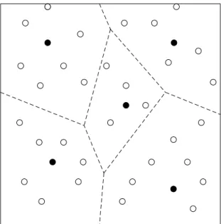
In recent years, researchers have proposed numer-ous clustering routing algorithms for WSNs to alleviate the hot spot problem. As the first proposed based on data fusion adaptive clustering topology protocol, Low-Energy Adaptive 3 Clustering Hier-archy (LEACH) [18] plays an important role in the development of clustering topologies routing pro-tocols. The survival time of the whole algorithm is expressed in rounds in LEACH, though cluster establishment and data communication periodically. Through the random election of cluster heads and the application of data fusion method to reduce the communication load, LEACH can extend the net-work’s survival time greatly. However, due to the random cluster head selection scheme, the problem of cluster head uneven distribution or the number of cluster members appears frequently, which is shown as Fig. 1. LEACH-Centralized (LEACH-C) [19] is proposed to solve the problem of uneven cluster head distribution, which select the cluster head by global information. However, the global optimal selection is an NP problem, which is difficult to draw the exact solution. LEACH-Energy (LEACH-E) [20] considers node residual energy to solve the hot spot problem in LEACH.
In the Power-Efficient GAthering in Sensor Infor-mation Systems (PEGASIS) [21], sensor nodes are constructed in a chain, with each node serving as the
Fig. 1. LEACH cluster protocol.
header of chain. Then, the data is transmitted along the chain to CHs and finally to the sink node.
A Hybrid Energy-Efficient Distributed (HEED) clustering protocol [22] considers the residual energy of the node in its clustered threshold. Here, the can-didate node is firstly generated, and then, formal CHs are selected according to the maximum residual energy and minimum reachable energy. However, the overhead for network clustering is inevitable due to the iterative manner in CH election.
Besides, other model [23] alleviates the hot spot problem via an unequal clustering manner. This algorithm assumes that two concentric circles are constructed with the sink node as their center. The cluster formed by the nodes in the inner circle is small, for which more energy is reserved for outer circle data forwarding. However, this model requires CHs are with powerful processing ability, and the locations of sensor nodes have to be obtained in advance. Another unequal clustering routing protocol, EnergyEfficient Uneven Clustering (EEUC) [24] divides the network into non-uniform clusters. However, the problem of cross-iteration and the node residual energy factors are not considered during the computation of radius.
3. Network model
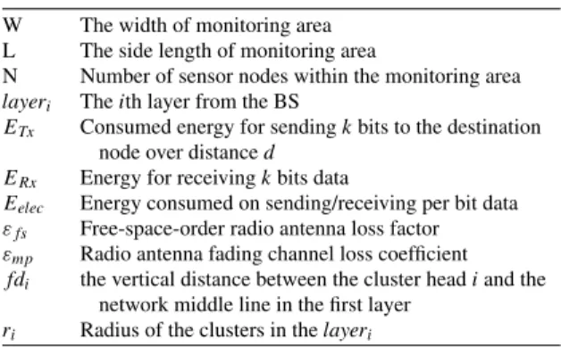
In this section, the network model is introduced. Table 1 summarizes the key notations used in the paper.
Table 1 List of notations W The width of monitoring area L The side length of monitoring area
N Number of sensor nodes within the monitoring area
layeri Theith layer from the BS
ETx Consumed energy for sendingkbits to the destination node over distanced
ERx Energy for receivingkbits data
Eelec Energy consumed on sending/receiving per bit data εfs Free-space-order radio antenna loss factor εmp Radio antenna fading channel loss coefficient fdi the vertical distance between the cluster headiand the
network middle line in the first layer
ri Radius of the clusters in thelayeri
3.1. Assumption
Wireless sensor network consists of target, sensing nodes, observation node and sensing field. In addi-tion, the external network, the user and the remote task management unit make the system description complete. The entire network scenario is shown in Fig. 2, the underlying application is for data collec-tion. We consider a W×L rectangular monitoring area, within which there are N sensor nodes and one sink node. The set of all nodes is given byS=
{s1, s2, . . . , sN−1, sN}, where|S| =N. Our design is based on following assumptions:
– All sensor nodes are randomly deployed in a two-dimensional plane within the monitoring area. A base station (referred to sink node) is located outside the area, while the locations of base station and sensor nodes are fixed. – Each sensor node is identified by a unique ID.
We assume all sensor nodes are initialized with the same amount of energy.
– Each sensor node can be either Cluster Header (CH) or Cluster Member (CM), depending on the design of routing protocol.
– The network time is decoupled into each round, within which sensor nodes will send their col-lected data to the base station.
– Each sensor node can calculate its coordi-nate away from the emission source, according to the intensity and angle of its received signal.
3.2. Energy consumption mode
The wireless communication energy consumption model is presented in [19] and is shown in Fig. 3. the energy consumptionETx(k, d) for data transmission perkbits, with a distancedbetween pairwise nodes, is calculated according to Equation (1):
Fig. 2. Network scenario.
ETX(k, d)=
k×Eelec+k×εfs×d2if (d <d0)
k×Eelec+k×εmp×d4else (1) Where the threshold value d0 can be calculated according to Equation (2):
d0=
εfs
εmp (2)
Here, Eelec represents the energy consumption of transmission circuit. Besides,εfsandεmprepresent the amount of energy required by power amplification in that two models.
On the one hand, if the transmission distance d
is smaller than the threshold d0, the energy ampli-fication consumption is based on free-space model. On the other hand, when the transmission distance is larger than or equal to threshold d0, the multi-path fading model is applied. It can be observed that, applying single hop transmission for long range data transmission is energy costly. Therefore, apply-ing multi-hop communication is alternatively more energy efficient.
4. Energy-balanced and unequally-layered routing protocol
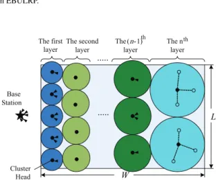
Design of EBULRP consists of three phases, which are: Cluster Formation Phase, Data Transmission Phase, and Cluster Maintenance Phase. The main idea of EBULRP is shown in Fig. 4. Here, the entire net-work topology is decoupled into n layers, where each layer is assigned with a given width. At each layer, the closer to the base station, the smaller that the radius of cluster is. In order to alleviate the hot spot problem, EBULRP balances the energy consumption among CHs, based on the design detailed in this section.
We assumed that the whole sensor network is divided into n layers with unequal width based on the distance to the base station, and the following properties can be obtained:
a) The closer to the base station, the smaller the width of the layer (WL), and the smaller the cluster radiusr;
b) The cluster size in the same layer is equal, and the cluster radius is half width of the corre-sponding layer;
c) The data transmission adopts the multi-hop communication mode from the upper layer to the next layer until the base station.
Fig. 4. Overview of cluster formation in EBULRP.
4.1. Cluster formation phase
(1) Radius of Cluster Calculation: Given thatrnis the radius of cluster at thenth layer, the set for that at all layers is then given byR= {r1, r2, . . . rn−1, rn}. By referring to Fig. 4, the corresponding width of a given layer is calculated by 2×rn, while the transmission range of CH at each layer is given by (rn+rn−1).
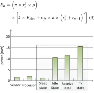
The energy consumption of each sensor node mod-ule is shown in Fig. 5. The energy consumption mainly concentrates on the wireless communication module. Send data state cost most energy, and the idle state consumption is almost the same to the receive state.
Given that a sensor node is with k bits data for transmission, the energy consumption En of CH at thenth layer for data transmission, is calculated as:
En= π×r2n×ρ × k×Eelec+εfs×k× rn2+rn−1 2 (3) Processor Sensor wireless communicaƟon Sleep state Idle State Receive State Tx state 0 5 15 20 10 power (mW)
whereρis the deployment density of sensor nodes. Regarding the CH at the (n−1)th layer, its energy consumptionEn−1is not only due to the data trans-mission within its local cluster, but also due to relaying the data from those CHs at the nth layer. Here, we have: En−1 =π×rn−2 1×ρ + π×r2n×ρ× L 2×rn × 2×rn−1 L ×k×Eelec+εfs×k×(rn−1+rn−2)2 (4) where L 2×rn
indicates the number of clusters at the nth layer. While
2×rn−1
L
is the reciprocal of the number of clusters at the (n−1)th layer. Note that L is the length of monitoring region shown in Fig. 4. Likewise, at the (n−2)th layer, the energy consumption of CH, as forEn−2, is given by:
En−2= π×rn−2 2×ρ + n i=n−1 π×ri2×ρ× L 2×ri × 2×rn−2 L ×Eelec×k+εfs×k×(rn−2+rn−3)2 (5) En =π×r2n×ρ × k×Eelec+εfs×k× rn2+rn−1 2 En−1 =π×r2n−1×ρ + π×r2n×ρ× L 2×rn × 2×rn−1 L ×k×Eelec+εfs×k×(rn−1+rn−2)2 (6) . . . . E1 =π×r12×ρ +n i=2 π×ri2×ρ× L 2×ri × 2×r1 L ×k×Eelec+εfs×k×R1 2
Based on above derivation, we can obtain Equation (6), whereR1as an approximate distance between the base station and the CH at the 1st layer, is calculated as:
R1= L 4
2
+dmin2 (7) Here,dminis the shortest distance from the mon-itoring area to the base station. In particular, aiming to balance the energy consumption of CHs, we have:
Ek ∼=Ek−1∼=. . .∼=E2∼=E1 (8) In addition, according to the characteristics of net-work structure,we can get:
r1+r2+. . .+rn−1+rn= W
2 (9)
Where,Wis the width of the monitor area. Then, from Equations (6) to (9),r1, r2, . . . , rncan be calcu-lated, and the width of each layer can be established. For example, we suppose a network structure consist-ing by only three layers,n=3. Then,r1, r2, . . . , r3 can be calculated as (10). ⎧ ⎪ ⎪ ⎪ ⎪ ⎪ ⎪ ⎪ ⎪ ⎪ ⎪ ⎪ ⎪ ⎪ ⎪ ⎪ ⎪ ⎪ ⎪ ⎪ ⎪ ⎪ ⎪ ⎪ ⎪ ⎪ ⎨ ⎪ ⎪ ⎪ ⎪ ⎪ ⎪ ⎪ ⎪ ⎪ ⎪ ⎪ ⎪ ⎪ ⎪ ⎪ ⎪ ⎪ ⎪ ⎪ ⎪ ⎪ ⎪ ⎪ ⎪ ⎪ ⎩ E3= π×r32×ρ ×Eelec×k+εfs×k×(r2+r3)2 E2= π×r22×ρ+ π×r23×ρ× L 2×r3 ×2×r2 L ×Eelec×k+εfs×k×(r1+r2)2 E1= π×r12×ρ + 3 i=2 π×r2i ×ρ× L 2×ri ×2×r1 L × Eelec×k+εfs×k×R1 2 E1∼=E2∼=E3 W 2 =r1+r2+r3 (10)
1 41 fd = r 2 21 fd = r 3 0 fd = 4 21 fd = r 5 41 fd = r W L Base Station Cluster Head min d 1 r ⋅⋅⋅⋅⋅
(a) N is an odd number
W L Base Station Cluster Head min d ⋅⋅⋅⋅⋅ 1 51 fd = r 2 31 fd = r 3 1 fd =r 4 1 fd =r 5 31 fd = r 6 51 fd = r 1 r (b) N is an odd number
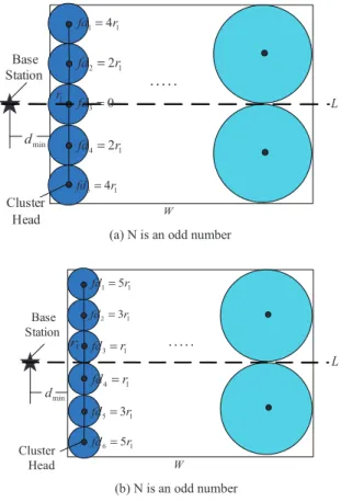
Fig. 6. The communication distance between each cluster head and the base station inLayer1.
In calculating the radius of the cluster, the data transmission distance of each cluster head in other layers, except the first layer, can be approximated as the sum of the cluster radius between adjacent layers. However, As shown in Fig. 6 (a) and (b), the base sta-tion is the next-hop data transfer for the cluster head in the first layer. the data transmission distance is not only the sum of the cluster radius between adjacent layers, and the distances between the respective base stations are also different. Assume thatNis the total number of cluster heads in the first layer. It can be an odd number or even number. fdi is the vertical distance between the cluster headiand the network middle line in the first layer.
For the first situation:Nis an odd number.
fdi= ⎧ ⎪ ⎪ ⎪ ⎨ ⎪ ⎪ ⎪ ⎩ [N−(2i−1)]×r1, i=1∼ N 2 +1 2 i− N 2 ×r1, i= N 2 +2 ∼N (11)
For the second situation:Nis an even number.
fdi= ⎧ ⎪ ⎪ ⎨ ⎪ ⎪ ⎩ [N−(2i−1)]×r1, i=1∼N 2 2 i−N 2 −1 ×r1, i= N 2 +1∼N (12) Then, the mathematical expectation or mean offdi,
E[fdi], is as follow:
E[fdi]= 1
N(fd1+fd2+. . .+fdN−1+fdN)
(13) Then, in Equations (6), The data transmission dis-tance between the cluster head and the base station in the first layer,R1, can be expressed as:
R1=
(r1+dmin)2+(E[fdi])2 (14) (2) Cluster Formation: The base station broadcasts a signal to the entire monitoring region, based on a given transmission power. Sensor nodes receiving this signal, then calculate their relative coordinates according to the intensity and the angle of signal [25]. Furthermore, based on the previous discussion on the radius of cluster, the base station can calcu-late all locations of Ideal CHs (namely ICHs) at each layer, based on a n layers’ topology configuration. Note that the locations of CHs finally determined in the network, may have a certain variation from that of ICHs calculated by the base station.
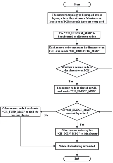
With a flowchart shown in Fig. 4, the detailed pro-cedure for cluster formation is listed as follows:
1) The base station broadcasts a message namely “CH INFORM MSG” including information about all ICHs at all layers, to sensor nodes in the entire network. Particularly, for each layer, it includes:
• The layer ID.
• The locations of all ICHs at certain layer. • The IDs of all ICHs at certain layer. • The radius of clusters at certain layer.
2) After receiving the “CH INFORM MSG”, a sensor node si, with the closest distance to a given ICH, initially elects itself as the CH for competi-tion. Besides,sifurther broadcasts a “CH COMPETE MSG” to its neighbors, including the layer ID, ID of ICH it elects for competition and its distance to that ICH.
3) Any other sensor node sj receiving this “CH COMPETE MSG”, will compare the information in relation to the ICH it elects for competition, with that of in this received message. If the same ICH is under
competition, all details included in “CH COMPETE MSG”, will be inserted into a set SCH.
4) After a given competition time interval, each sensor node will compare the distance to the ICH it competes, with those values inSCH. Here, the sen-sor node making comparison is elected as the CH, only if it is with the smallest value regarding such distance metric. Followed by this successful election, that given sensor node then broadcasts a “CH ELECT MSG”.
5) Other sensor node receiving “CH ELECT MSG”, will join the closest cluster by sending a “CH JOIN MSG”. Here, the estimation regarding the closest cluster is based on the intensity of signal. In
special case, the sensor node without “CH ELECT MSG” received, will alternatively broadcast “CH FIND MSG” to find the closest CH and join that cluster.
6) The network clustering is finished until all CHs are elected, around which other sensor nodes are their CMs.
4.2. Data transmission phase
In EBULRP, the data transmission is decoupled into two stages:
In the first stage, the data transmission happens between the CH and its CMs.
Fig. 8. Time slots in EBULRP.
The data transmission in the second stage is between CHs and base station. Here, two com-munication modes are applied. The single-hop communication is for directly delivering data from the CH to the base station. The multi-hop commu-nication is for intermediate data transmission to the base station, through a number of CHs. Note that we already discussed that using multi-hop communica-tion is more energy efficient in Seccommunica-tion 3.
As shown in Fig. 7, the network time is decoupled into several rounds, where each round consists of sev-eral time slots. The time slots in EBULRP is shown in Fig. 8. Based on different characteristics, these time slots are classified into:
• CM-Slot: The time slot assigned for CM, to report its request and transmit data to the CH. • Control-Slot: The time slot to manage the
cluster.
• CH-Slot: The time slot assigned for CH, to deliver data to the base station.
• Special-Slot: The time slot assigned to directly receive the information broadcasted from the base station.
1) First Stage: For the first stage, EBULRP mod-ifies the fixed time slot based communication as adopted by LEACH, into a dynamic time slot based communication. It is highlighted that such modifica-tion can meet the requirement of different CMs with certain time slot for data transmission.
Starting from the first CM-Slot, each CM sends request in relation to its number of required time slots for data transmission. Upon receiving requests from all CMs within the local cluster, the CH then ran-domly allocates the remaining CM-Slots, such that each node with pending request is allocated with at least one CM-Slot.
Before the expiration of first CM-Slot, the CH will inform other CMs regarding their specific assigned CM-Slots. Each CM will only return to awake mode upon an arrival of its own CM-Slots, and then starts to transmit data to the CH. In other time slots, CMs will remain in sleep mode for energy saving purpose.
... W L ... The first layer Base Station Cluster Head The second layer layer The (n- 1)th layer The nth
Fig. 9. The inter-layer multi-hop communication mode.
2) Second Stage: Upon the collection of data, the CH will then deliver data to the based station, via multi-hop communication mode, only within the CH-Slot. Given that the network clustering has already been established, the neighbor information is exchanged between adjacent CHs, and stored locally for selecting the next hop. Overall, the data is relayed from the CH at an upper layer to that at a lower layer, and finally from the CH at the lowest layer to the base station. If there are more than one CHs available for next hop, the one with a closer distance and more energy is selected as the next hop. This aims to bal-ance the energy consumption among CHs, as such the hop spot problem can be alleviated. In special case, a direct data transmission is established with the base station, if there is no available next hop.
With further concerning, the Direct Sequence Spread Spectrum (DSSS) can be integrated into this multi-hop communication. By doing so, each cluster is coded with different SS in order to avoid crosstalk. The signal from other clusters will not be filtered by CMs in their local cluster. This can effectively alleviate the interference across CMs in adjacent clusters. Furthermore, the Carrier Sense Multiple Access (CSMA)mechanism can be applied for communication between CHs, and that between CHs and the base station. Here, CHs should listen to the channel before data transmission, to prevent collision, as shown in Fig. 9.
4.3. Cluster maintenance phase
Basically, CHs are responsible to manage their CMs within the cluster, along with data forwarding for intra-cluster and inter-cluster data forwarding. In the worst case, CHs may run out of energy.
Indeed, clustering based routing protocols such as LEACH and EEUC, rely on periodical re-clustering mechanism to balance the energy consumption of CHs. However, such re-clustering mechanism requires huge information exchange and complicated computation, which limits the system scalability.
Our design in EBULRP is not with such periodical re-clustering mechanism. Instead, each CM within a cluster will be elected as the CH alternately. Once a CM becomes the CH, it will collect the information in relation to an average energyEavgof other CMs in the cluster. Whenever the CH detects that its energy is smaller than Eavg2 or a thresholdEmin, it considers
Fig. 10. The cross-layer communication in EBULRP.
itself not to be the CH anymore. Upon this decision, within the Control-Slot, the CH collects the infor-mation in relation to the energy of other CMs in the cluster, and elects the one with the highest energy as the CH in next round.
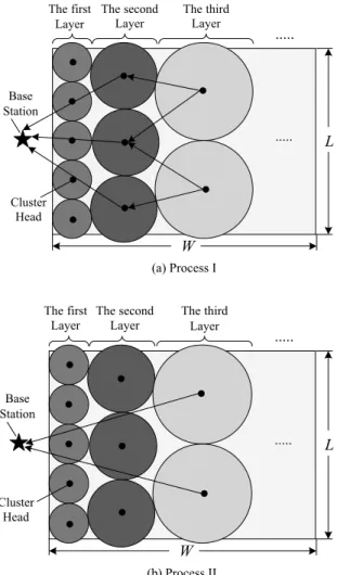
As previously mentioned, EBULRP is layered with different width, where the width and clusters at cer-tain layer are decreased, from the layer that is with the fastest distance to the base station. In case that sensor nodes are uniformly distributed in the network, the cluster with a smaller radius thereby consists of less number CMs. In the worst case, all nodes including CHs and CMs at a given layer may run out of energy, however those at other layers still work.
In EBULRP, a cross-layer communication is applied to prolong the network lifetime. Here, the base station will inform those CHs at an upper layer to directly communicate with itself, if all nodes at a lower layer run out of their energy. For example, if all nodes at the 1st layer are energy exhausted, all nodes at the 2nd layer then performs direct communication with the base station, as shown in Fig. 10(a) and (b).
5. Performance evaluation
The scenario comprises a 150 m by 120 m monitor-ing area. The performance is evaluated usmonitor-ing Matlab, with the configuration listed in Table 1. In order to show the advantage of our proposal, we also imple-ment the LEACH [18], EEUC [24] for comparison. Three evaluation metrics of the network performance have been studied as follows:
• Network Lifetime: There is no universally
agreed definition for the network lifetime. The importance of WSNs is to be operational and able to perform tasks. In WSNs, it is important to maximize the network lifetime, which means to increase the network survivability or to pro-long the battery lifetime of sensor nodes. Here, the total number of alive nodes is applied in our evaluation to measure the network lifetime.
• Network Energy Balance: This metric
cal-culates the variance of the CHs’ energy consumption in each round, to evaluate the energy balance in the network.
• Average Energy Consumption: This metric
shows the average dissipation of energy per node over time in the network as it performs various functions such as transmitting, receiving, sens-ing and aggregation of data.
Table 2 Simulation configuration
Parameter Value
Network Coverage Area 180 m×120 m Location of Base Station (–50, 60) Number of Sensor nodes 180
Initial Energy 0.5 J Eelec 50 nJ/bit εfs 10 pJ/bit/m2 εmp 0.0013 pJ/bit/m4 Network Layer 2 r1 30.62 m r2 44.38 m
Data size 3000 bits
Table 3
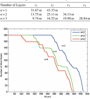
Configuration based on different layers
Number of Layers r1 r2 r3 r4
n= 1 31.67 m 43.33 m
n= 2 13.75 m 25.11 m 34.13 m
n= 3 9.74 m 16.52 m 19.90 m 28.84 m
Fig. 11. Influence of layers.
The parameters used in the simulation experiments are shown in Table 2. To begin with, the influence of network layers is evaluated. Table 3 shows the radius of cluster with layers of 1-layer, 2-layers, 3-layers for the design of EBULRP, respectively. Note that more or less hops will lead to additional communication overhead, so the number of network layers has a sig-nificant impact on the overall network performance.
Figure 11 shows the network lifetime of EBULRP with 1-layer, 2-layers and 3-layers configuration respec-tively, where the radius of cluster at each layer follows calculation in Table 2. In case of 2-layers,nodes can survive longer and show better performance than other two cases. Therefore, it is essential for the base station to determine an appro-priate layer when designing the cluster structure.
Fig. 12. Average energy consumption of nodes. Figure 12 shows the average energy consumed by all nodes, at the first 100 rounds. The node energy consumption of LEACH is significantly higher than that of EEUC and EBULRP. The reason is that LEACH makes use of single-hop data transmis-sion for inter-cluster communication, which results in more energy consumption at CHs which are far from the base station. While EEUC builds the topol-ogy through unequal clustering method, along with a multi-hop communication to reduce the commu-nication cost during the routing selection. However, due to the random distribution of clusters, there still exists uneven distribution which may cause abun-dant hops during inter-cluster data transmission. In contrast, EBULRP lets the base station to proceed main computation for network clustering, and only leaves a littledata exchange and calculation at sensor nodes. Furthermore, it achieves an even distribution on clusters where the number of hops for inter-cluster data forwarding is relatively fixed. Such a way better organizes the network clustering for energy saving purpose.
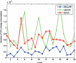
Since the core idea is to alleviate the hot spot problem, the accuracy of computation on network-clustering plays an important role in energy balance. In Fig. 13, we arbitrarily select 20 rounds of data to calculate the variance of the CHs’ energy con-sumption. Here, EBULRP achieves the smallest variation,followed by EEUC and LEACH. This is because that the design of EBULRP considers the properties of different CHs, and well organizes the network topology to address the energy unbalance among CHs.
The purpose of Fig. 14 is to examine the network lifetime. It shows the number of the alive nodes along
Fig. 13. Variations of CHs’ energy consumption.
Fig. 14. Number of alive nodes.
with the number of rounds. If considering that 50% of sensor nodes are dead, EBULRP, EEUC and LEACH end at 467, 338 and 250 rounds respectively. Here, the performance of EBULRP is 38% higher than EEUC and 87% higher than LEACH. If considering 80% of sensor nodes are dead, EBULRP, EEUC, and LEACH end at 562, 441, and 398 rounds respectively. Here, the performance of EBULRP is 27% higher than EEUC and 41% higher than LEACH. This is due to that EBULRP adopts a well clustering and multi-hop communication for inter-cluster data transmission.
6. Conclusion
We have proposed EBULRP in this article to solve the hot spot problem. The design of EBULRP alleviates the computation complexity at CH side, via
a less numbers of controlling information exchange. We firstly analyzed the energy consumption of CHs, then established a multi-layered network structure to balance the energy consumption among CHs. Com-pared with the previous works LEACH and EEUC, results show EBULRP significantly prolongs the net-work lifetime and balances the energy consumption in the network.
Acknowledgments
This paper is supported by the National Natu-ral Science Foundation (61102105), the PostdoctoNatu-ral start foundation of Heilongjiang Provence (LBH-Q12117); the Foundation for Innovative Research of Harbin (2015RAQXJ008); and the Fundamen-tal Research Funds for the Central Universities (GK2080260138 ). We Also would like to acknowl-edge the support of the University of Surrey 5GIC (http://www.surrey.ac.uk/5gic) members for this work.
References
[1] J. Yao, S. Feng, X. Zhou and Y. Liu, Secure routing in multihop wireless Ad-hoc networks with decode-and-forward relaying,IEEE Transactions on Communications
64(2) (2015), 753–764.
[2] Y. Cao, Z. Sun, N. Wang, M. Riaz, H. Cruickshank and X. Liu, Geographic-based spray-and-relay (GSaR): An effi-cient routing scheme for DTNs,IEEE Transactions on Vehicular Technology64(4) (2015), 1548–1564.
[3] A. Zanella, A. Bazzi, G. Pasolini and B.M. Masini, On the impact of routing strategies on the interference of ad hoc wireless networks,IEEE Transactions on Communications
61(10) (2013), 4322–4333.
[4] T. Wang, C. Zhao, H. Xu and J. Qi, An intelligent processing model on heterogeneous information from the internet of things,Journal of Computational Information Systems7(2) (2011), 578–584.
[5] S. Kurt, H.U. Yildiz, M. Yigit, B. Tavli and V.C. Gungor, Packet size optimization in wireless sensor networks for smart grid applications,IEEE Transactions on Industrial Electronics64(3) (2016), 2392–2401.
[6] A.A. Rahat, R.M. Everson and J.E. Fieldsend, Evolution-ary multi-path routing for network lifetime and robustness in wireless sensor networks,Ad Hoc Networks52(2016), 130–145.
[7] H.Y. Kim, An energy-efficient load balancing scheme to extend lifetime in wireless sensor networks,Cluster Com-puting19(1) (2016), 279–283.
[8] T. Wang, Y. Zhang, Y. Cui and Y. Zhou, A novel protocol of energy-constrained sensor network for emergency monitor-ing,Interational Journal of Sensor Networks15(3) (2014), 171–182.
[9] H. Echoukairi, K. Bourgba and M. Ouzzif, A Survey on Flat Routing Protocols in Wireless Sensor Networks,Advances
in Ubiquitous Networking. Springer Singapore, 2016, pp. 270–277.
[10] J. Kulik, W. Heinzelman and H. Balakrishnan, Negotiation-based protocols for disseminating information in wire-less sensor networks, Wireless Networks 8(2) (2002), 169–185.
[11] C. Intanagonwiwat, R. Govindan and D. Estrin, Directed diffusion for wireless sensor networking,IEEE/ACM Trans-action on Networking11(1) (2003), 2–16.
[12] T. Wang, J. Wu, H. Xu, J. Zhu and M. Charles, A cross unequal clustering routing algorithm for sen-sor network,Measurement Science Review13(4) (2013), 200–205.
[13] M. Kavitha, B. Ramakrishnan and R. Das, A novel routing scheme to avoid link error and packet dropping in wire-less sensor networks,International Journal of Computer Networks and Applications (IJCNA)3(4) (2016). [14] J. Yan, M. Zhou and Z. Ding, Recent advances in
energy-efficient routing protocols for wireless sensor networks: A review,IEEE ACCESS4(2016), 5673–5686.
[15] Y. Du, S. Yang and R. Zhang, Design of an intrusion detec-tion system for wireless sensor networks,Sensor Letters
9(5) (2011), 2082–2086.
[16] R. Zhu, Efficient fault-tolerant event query algorithm in dis-tributed wireless sensor networks,International Journal of Distributed Sensor Networks5(4) (2010), 1–7.
[17] S. Zou, W. Wang and W. Wang, A routing algorithm on delay-tolerant of wireless sensor network based on the node selfishness,EURASIP Journal on Wireless Communications and Networking1(2013), 1–9.
[18] W. Heinzelman, A. Chandrakasan and H. Balakrishnan, Energy-Efficient Communication Protocols for Wireless Microsensor Networks,IEEE Hawaii International Con-ference on Systems Sciences (HICSS), 18, 2000, p. 8020. [19] W. Heinzelman, Application-Specific Protocol
Architec-tures for Wireless Networks, Massachusetts Institute of Technology, 2000.
[20] D. Peng and Q. Zhang, An energy efficient cluster-routing protocol for wireless sensor networks,IEEE International Conference on Computer Design and Applications (ICCDA)
2(2010), 530–533.
[21] S. Lindsey, C. Raghavendra and K. Sivalingam, Data gath-ering algorithms in sensor networks using energy metrics, IEEE Transactions on Parallel and Distributed Systems
13(9) (2002), 924–935.
[22] O. Younis and S. Fahmy, Heed: A hybrid, energy-efficient, distributed clustering approach for Ad hoc sensor networks, IEEE Transcations on Mobile Computing 3(4) (2004), 366–379.
[23] S. Soro and W. Heinzelman, Prolonging the lifetime of wire-less sensor networks via unequal clustering,IEEE Computer Society Press(2005), p. 556.
[24] C. Li, M. Ye, G. Chen and J. Wu, An Energy-Efficient Unequal Clustering Mechanism for Wireless Sensor Net-works,IEEE International Conference on Mobile Ad-hoc and Sensor Systems (MASS), 2005, p. 604.
[25] A. Parameswaran, M.I. Husain and S. Upadhyaya, Is RSSI a Reliable Parameter in Sensor Localization Algorithms,An Experimental Study, Field Failure Data Analysis Workshop (F2DA2009). 2009, p. 5.