Mechanistic Probability
∗
(Synthese, 187(2), 2012. Accepted October 2010.)Marshall Abrams
Department of Philosophy
University of Alabama at Birmingham
900 13th Street South, HB 414A
Birmingham, AL 35294-1260
[email protected]
August 7, 2012
Abstract
I describe a realist, ontologically objective interpretation of probability, “far-flung frequency (FFF) mechanistic probability”. FFF mechanistic probability is defined in terms of facts about the causal structure of devices and certain sets of frequencies in the actual world. Though defined partly in terms of frequencies, FFF mechanistic probability avoids many drawbacks of well-known frequency theories and helps causally explain stable frequencies, which will usually be close to the values of mechanistic probabilities. I also argue that it’s a virtue rather than a failing of FFF mechanistic probability that it does not define single-case chances, and compare some aspects of my interpretation to a recent interpretation proposed by Strevens.
∗I’m grateful to the following people for feedback and conversations concerning various presentations and unpublished work which led up to this paper: Scott Anderson, Erik Angner, Andre Ariew, Murat Aydede, Prasanta Bandyopadhyay, Frederic Bouchard, Robert Brandon, Jason Bridges, Patrick Forber, Matt Frank, Dan Garber, Alan Hajek, Christopher Hitchcock, Carl Hoefer, Larry James, Richard Johns, Michael Katz, Harold Kincaid, John Kulvicki, Aaron Lercher, Aidan Lyon, Ruth Millikan, Samir Okasha, Jim Otteson, John Pollock, Stewart Rachels, Richard Richards, Alex Rosenberg, Don Ross, Eric Schliesser, Elliott Sober, Michael Strevens, Julio Tuma, Paul Weirich, Greg Wheeler, Bill Wimsatt, Chase Wrenn, audience members at talks, students in a seminar at Duke University, and some very helpful anonymous reviewers. None of these people should be assumed to agree with, or even be sympathetic to what follows.
1 Introduction 1
1.1 The need for new interpretations of probability . . . 2
1.2 Must an interpretation define chances? . . . 3
1.2.1 How many chances are there? . . . 3
1.2.2 There are few fat chances . . . 4
2 Preliminaries 5 2.1 The wheel of fortune . . . 6
2.2 Concepts and terminology . . . 6
2.3 Strategy . . . 8
3 Role of the microconstancy inequality theorem 8 3.1 The theorem . . . 9
3.2 Adjusting input measures . . . 10
3.3 Application to construction of an interpretation . . . 11
4 Justification of an input measure 11 4.1 On Strevens’ input measure . . . 12
4.2 Natural collections of inputs . . . 13
4.3 Constructing the input measure . . . 14
5 FFF mechanistic probability 15 5.1 Summary of the interpretation . . . 15
5.2 Bubbles relative to natural collections . . . 16
5.3 Consequences of bubbliness . . . 18
5.4 Causal aspects of FFF mechanistic probability . . . 21
5.5 Epistemological considerations . . . 21
5.5.1 On evidence for mechanistic probability . . . 21
5.5.2 On evidence from mechanistic probability . . . 22
5.6 Other issues . . . 22 5.6.1 Independence . . . 22 5.6.2 Reference classes . . . 23 5.6.3 Indeterminism . . . 23 5.6.4 Precision . . . 23 6 Conclusion 24 A Microconstancy inequality theorem 25 A.1 Theorem . . . 25
1
Introduction
While the meaning of “probability” in mathematics is provided by a few closely related sets of axioms, uses of “probability”, “chance”, and related terms in science and everyday life seem to require more than satisfaction of such axioms. For example, if the surface of a table is divided into regions,1 each region’s proportion of the table top can count as its probability from a mathematical point of view: the axioms are satisfied. However, most uses of “probability” outside of a purely mathematical context would not count proportion of a table top as probability. Specifying what more than satisfaction of the axioms is needed is the problem of providing an “interpretation of probability”. Well-known interpretations of probability have serious defects or seem satisfactory for some purposes but not for others.
The goal of this paper is to outline a new interpretation of probability, one which is objective in the sense that the resulting probabilities are constituted only by facts about states of the world, without regard to epistemic factors such as belief or justification. Mechanistic probability—or more specifically what I call “far flung frequency (FFF) mechanistic probability”—defines probabilities of outcomes in terms of a kind of complex causal structure for what I call “causal map devices”, and very general facts about actual frequencies of inputs to similar devices.2
FFF mechanistic probability is not designed to interpret all scientific and everyday uses of “prob-ability” and similar terms. FFF mechanistic probability exists only when certain conditions are met. Other interpretations—some perhaps not yet devised—will be appropriate in other contexts. Various authors have proposed that one or another interpretation of probability could function as
the appropriate interpretation of probability for most worldly uses of “probability”, or for the more limited class of objective senses of the term. It’s not clear to me why an all-purpose interpretation of probability is needed. Probability fills different roles in different contexts, and the material bases of phenomena that seem to involve probabilities could vary.
I’ll begin with a quick overview of some advantages and disadvantages of other interpretations of probability in order to motivate mechanistic probability’s special features, concluding with a list of desiderata which I believe one or more interpretations of probability ought to satisfy (§1.1). Since some readers may feel that it is problematic that mechanistic probabilities are never single-case, I then include a brief discussion of the roles of single-case objective probabilities and why it might be advantageous to avoid defining them in some interpretations (§1.2). Next, after introducing an example and terminology which will be used in the rest of the paper (§2), I summarize a “micro-constancy inequality theorem” (proved in the appendix) and its role in defining FFF mechanistic probability (§3). Section 4 addresses the main challenge that must be dealt with by a mechanistic interpretation of probability, namely providing a naturalistic specification of a measure over initial conditions. Section 5 summarizes and refines the resulting interpretation of probability, clarifies its properties, and discusses some potential difficulties. The concluding section summarizes advan-tages and disadvanadvan-tages of FFF mechanistic probability. Finally, the appendix states and proves the microconstancy inequality theorem.
1Regions which are not too mathematically bizarre, i.e. which are measurable—see e.g. (Friedman, 1982, Ch. 1) for an illustration.
2Mechanistic probability is inspired by work by Poincar´e (1912,§91) on the method of arbitrary functions and is based partly on work by Strevens (2003; 2005), though the main ideas were developed before I had read Strevens’ work (Abrams, 2000).
1.1
The need for new interpretations of probability
Brief descriptions of a few prominent interpretations and some apparent virtues and drawbacks will help to clarify the context and motivation for my proposal. I make no pretense of providing a proper presentation and critique of these interpretations, which has been done by others.3
First, traditional finite frequency interpretations take probabilities to be relative frequencies in actual sets of occurrences; this, however, allows probabilities to deviate from values which their conceptual role requires. For example, we might think the probability of heads for tosses of a fair coin is 12, but the frequency of heads in actual, finite sets of tosses rarely takes precisely that value, and in fact varies from 0 to 1 in different sets of tosses. Without recourse to an additional interpretation of probability in order to justify laws of large numbers, it’s not even clear why we should expect the frequency of heads to be close to 12. An alternative is to claim that probabilities are long-run hypothetical frequencies, i.e. what a frequency would settle down to in the limit if the number of trials were extended indefinitely, but again, it’s not clear why we should expect frequencies to take the intuitively correct values. Thus simple frequency theories do not justify values for probabilities that are even close to the values needed in many uses of probability in science and everyday life.4
More importantly, it seems that some scientific and practical uses of probability require that probability cause or explain stable frequencies—the fact that certain contexts usually produce particular frequencies of outcomes; simple frequency theories cannot do this. This is also a reason that I think it’s worth exploring alternatives to Best System Analysis chances (Lewis, 1980, 1994; Loewer, 2001, 2004; Hoefer, 2007): Best System probabilities sometimes depend on whatever the frequencies happen to be, without requiring that these frequencies have any causal explanation at all.5 Similarly, although I believe that Bayesian interpretations (e.g. (Earman, 1992; Howson and Urbach, 1993; Williamson, 2010)) are useful in various contexts, they aren’t designed to explain frequencies.
As suggested above, I take the view that different interpretations of probability are appropriate for different contexts. On this view, it would be a mistake to assume that requirements for appli-cation of an interpretation are automatically met whenever probabilities are usefully postulated in certain scientific or practical contexts (as is advocated by Sober (2010), and sometimes in the con-text of Best System approaches (e.g. (Glynn, 2010)). To view objective probabilities as convenient place-holders is to leave them mysterious, and to give up on the possibility, at least sometimes, of explaining frequencies as general phenomena.
Propensity interpretations identify probabilities with a sort of generalized disposition to produce outcomes in varying degrees or in varying frequencies. As such, propensities potentially provide causal explanations for frequencies. However, propensities have many problems (Eagle, 2004). My view is that at best, propensities provide an interpretation of probabilities at the lowest physical level, i.e. for indeterminism in quantum mechanics (see Section 1.2.2).
Unlike these well-known interpretations, FFF mechanistic probability shows how it’s possible for objective probability to explain frequencies, at least in part, without explaining, determining, 3(H´ajek, 2009b) and (Gillies, 2000), among others, provide useful overviews of a variety of interpretations of probability and their advantages and disadvantages.
4See (H´ajek, 1996, 2009a) for a discussion of these and other drawbacks of frequency theories.
5This is true, for example, of Hoefer’s (2007) “third way” interpretation of probability, even though it makes probabilities depend on actual frequencies in the world in a complex way, as FFF mechanistic probability does, and even though many third way probabilities will depend partly on “statistical nomological machines” like the bubbly causal map devices which I describe.
governing, etc. outcomes on single trials (cf. §1.2, which explains why I view this as an advantage of mechanistic probability). Mechanistic probability is, in fact, consistent with both determinism and non-trivial chances6 which can be justified using another interpretation of probability. And though defined partly in terms of actual frequencies, FFF mechanistic probability avoids the most serious problems of simple frequency theories.
An interpretation of probability should satisfy specifiable constraints or desiderata, but there is no agreement on which constraints are essential. However, on the view that different interpretations of probability are suitable for different purposes, this divergence may be healthy. As the preceding discussion suggests, I take the following list of desiderata to be worthy of satisfaction:
Satisfaction of probability axioms
The probabilities satisfy a standard set of axioms including, at least, finite additivity.7 Ascertainability
It is in principle possible to discover what values probabilities have. Objectivity
The probabilities are constituted only by facts about states of the world, without regard to epistemic factors such as belief or justification. Thus, construction of an interpretation of probability requires that we provide naturalistic, non-epistemic definitions of all of its components.
Explanation of frequencies
That the probability of an outcomeA has the value it does should help explain why relative frequencies ofA tend to have similar values.
Distinguishing nomic regularities
A closely related desideratum is that an interpretation of probability be able to distinguish accidental from nomic regularities in frequencies (Strevens, 2011).
I argue below that FFF mechanistic probability satisfies these desiderata well enough to be valuable.
1.2
Must an interpretation define chances?
Some readers may feel that an objective interpretation of probability must be able to define single-case objective probabilities, or chances, so I’ll indicate here why I disagree.
1.2.1 How many chances are there?
It appears that there are three main, overlapping roles which single-case probabilities must play. First, single-case probabilities routinely guide individual action, whether involving games of chance or choices about where to wait for a bus. What’s needed for decisions, however, are only internal probabilities such as Bayesian credences, and it’s not clear that chances are needed to 6By “chance” I mean nothing more than “single-case objective probability”; no association with any particular strategy or interpretation is intended.
7Or should at least satisfy axioms that are recognizably similar to standard axioms (e.g. (Fetzer, 1981; Walley, 1991)).
justify them. For example, Dutch book arguments that degrees of belief concerning single cases should satisfy standard axioms can be based on frequencies without assuming chances.8
Second, single-case probabilities are required in order to prove laws of large numbers, often thought to justify assumptions about frequencies. However, most laws of large numbers cited to justify claims about frequencies only make claims about what happens in the limit. Their proofs may have implications about probabilities of various frequencies in finite sets, but note that FFF mechanistic probability justifies claims about finite frequencies directly, without chances.9
Third, single-case probabilities are routinely used in science, for example in statistical inference. However, consistent with remarks above, it seems problematic to infer the existence of chances from the mere fact that single-case probabilities seem to play certain crucial roles in successful science (e.g. (Sober, 2010; Hoefer, 2007; Glynn, 2010)). In particular, while I think there may be some chances to which which some fundamental physical theories refer, I’m sceptical of claims that propositions in special sciences refer to chances.
Note that there are many models but few (if any) laws in the special sciences. Given a model which has been successfully applied, questions typically remain about which aspects of the model correspond to, or approximate aspects of the world. Like other aspects of models, single-case probabilities assumed in models may well be mere conveniences which don’t correspond directly to anything in the world.10Thus further arguments concerning processes in the system modeled would be needed to justify claims that model probabilities refer to chances. Even if a proposition involving single-case probabilities were reasonably viewed as a special science law, the claim that these represent chances can’t necessarily be inferred from the law; special science laws don’t de-scribe fundamental reality in the way that some laws in physics do, and what’s important in the formulation of the law might not be the assumption that probabilities are single-case. A claim that what appear to be single-case probability terms in fact refer to chances would need to be justified by investigation into the way in which these terms are used and/or the underlying processes which give rise to phenomena described by the law. (See also §5.6.1.)
1.2.2 There are few fat chances
Let us call something a “fat chance” if it is not merely an objective single-case probability, but one in which the probability captures a matter of degree of strength concerning the connection between cause and effect—where this connection is understood in a realist, non-Humean sense. (Propensities are fat chances on some interpretations, but I don’t want to restrict the notion of a fat chance to any particular interpretation.)
A number of authors appear to claim that the chance of a particular outcome of a given cause event can have multiple values by relativizing chance to levels or properties or descriptions (e.g. (Mellor, 1971; Sober, 2010; Hoefer, 2007; Glynn, 2010)). I’ll argue that this cannot be so for fat chances. I think the argument captures a common intuition whose rationale has not been spelled out explicitly in this way.11
8Arguments in (Howson and Urbach, 1993, p. 344) and (Williamson, 2010, p. 41) can be adapted for this purpose.
9There are some theorems which specify rates of convergence of frequencies in terms of intervals which are not qualified with probabilities, but it seems to me that they apply to narrower ranges of situations than mechanistic probabilities does (cf. discussion in note below about Engel’s work).
10Cf. (Wimsatt, 2007) on the utility of false models.
11The argument is a generalization of one in (Abrams, 2007) and bears analogies to Kim’s causal exclusion argument (Kim, 1998) and to some arguments in (Schaffer, 2007). Intuitions related to my conclusion can
Whether fat chances exist or not, causal relations come in at least two strengths. If event c is such that it would definitely cause an instance of outcome A, let us say that the relation has strength 1. And we can call the absence of a causal relation, occurring when c is not such that it could cause anA, a (degenerate) causal relation of strength 0. Note that particular event ccannot bear causal relations of both strengths to A, which would mean that c both definitely would and definitely would not cause an A.
Suppose that there are fat chances, so that the causal relation is sometimes a matter of degree of strength between 0 and 1. Following the occurrence of c, some member A of a partition of outcomes will be realized as a result of c, even thoughcdoes not cause Awith strength 1.12 Then, just as c cannot cause A with strengths 0 and 1, it cannot cause A with strengths r and swhere r̸=s. On a non-Humean view of causal relations, to claim that a causal relation between an event and the realization of an outcome is simultaneously of multiple strengths seems at the very least counterintuitive, and in need of defense in terms of special assumptions about causal relations. (I don’t know what those assumptions could be.) An epistemological application may help to convey the point: If you knew that c caused A with strengths near 0 and near 1, should you expectA to occur oncec takes place?
This means, though, that fat chances of a possible outcome of a single cause cannot be relativized to distinct levels, properties, or descriptions. For example, consider a game in which a fair coin is flipped in order to choose which of two pairs of dice is to be tossed next. Both pairs of dice are loaded, but in different ways. Then a particular toss of a pair of dice cannot have one fat chance of double-six as a realizer of the propertybeing loaded toward double-sixand another fat chance of double-six as realizing toss of a pair of dice chosen by coin flip in such and such game setup. The toss is the same event regardless of what properties we focus on or how we describe it. There is a physical causal relation between the circumstances of the toss and the outcome double-six, and this causal relation cannot have multiple strengths.
This is not to say that there can’t be different objective, causal probability values for an outcome relative to different properties; however, these cannot all be single-case probabilities from the same cause event. (Mechanistic probabilities are not single-case, so they don’t conflict with determinism or with fat chances.)
In sum, my interpretation of probability will not define single-case probabilities, but there is not a compelling reason that it need do so (§1.2.1), and there is a compelling reason that it should not do so (§1.2.2). (I don’t see a consistent way that it could do so, without simply conjoining another interpretation.)
2
Preliminaries
I’ll assume in most of this paper that the world is deterministic, because determinism is the hard case: If we can justify a useful interpretation of probability under determinism, it is not difficult to add indeterminism to the picture (§5.6.3).
be found expressed in various places, including (Sklar, 1970) and (Lewis, 1986b). Such intuitions probably motivate the view that propensities are conditioned on the entire state of the universe or relevant light cone (Miller, 1994; Fetzer, 1981). In theory, Humeans should be unaffected by my argument, since they would not countenance fat chances.
Figure 1: x: velocity;y: spins; gray areas: red frequencies; black areas: black frequencies.
2.1
The wheel of fortune
There are some devices—including many games of chance—whose causal structure is such that it typically matters very little what pattern of inputs the device is given in repeated trials; the pattern of outputs is generally about the same. For example, a wheel of fortune with red and black wedges—a simplified roulette wheel—is a deterministic device: The angular velocity with which it’s spun completely determines whether a red or black outcome will occur. Nevertheless, if the ratio of the size of each red wedge to that of its neighboring black wedge is the same all around the wheel, then over time such a device will generally produce about the same frequencies of red and black outcomes, no matter whether a croupier tends to give faster or slower spins of the wheel. Why?
The wheel of fortune divides a croupier’s spins into small regions (“bubbles” below) within which the proportion of velocities leading to red and black are approximately the same as in any other such region (Figure 1). As a result, as long as the density curve of a croupier’s spins within each bubble is never very steep, the ratio between numbers of spins leading to red and leading to black within each bubble will be roughly the same. The overall ratio between numbers of red and black across all spins will then be close to the same value. In order for frequencies to depart from this value, a croupier would have to consistently spin at angular velocities narrowly clustered around a single value, or produce spins according to a precisely periodic distribution.
2.2
Concepts and terminology
We can give a more general, mathematical justification for the explanation of the stability of frequencies produced by devices like the wheel of fortune; this will provide a basis for a mechanistic interpretation of probability. I begin by defining a number of useful terms. I’ll use an upper bar (A) to represent negation/complementation.
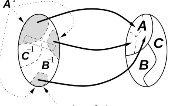
Call a device like the wheel of fortune, by which a set of possible initial conditions (inputs) produces instances (outputs) within an algebra of outcomes a causal map device (Figure 2); the function from initial conditions to outcomes which it realizes is a causal map. I’ll usually assume below that causal map devices are deterministic. Outcomes are (perhaps empty) disjunctions of members of a finite partition of basic outcomes. An outcome-inverse of initial conditions for a given outcomeA is a set of initial conditions all of which would produce the same outcomeA; an outcome-inverse set for A need not include all of the initial conditions which produceA, however. LetA−1 be that outcome-inverse set forA which does include all ofA’s possible causes.
1 −1 1 − −
C
B
input space output spaceB
A
an outcome inverse for
A
A
C
Figure 2: Structure of a causal map device. Heavy arrows summarize some causal relations.
For a causal map device, a bubble is a region in the input space containing points leading to all basic outcomes, i.e. containing outcome-inverse sets for each basic outcome (as a soap bubble reflects its surroundings). For example, the small dotted rectangle in Figure 2 is a bubble. A partition of the entire space of possible inputs into bubbles is a bubble partition.13 For the time being one can also assume that each bubble is a set of contiguous points which is not too bizarrely shaped (thus assuming the input space has a metric14). In the end these additional assumptions will not be required (§§5.1, 5.2), but making them now will allow simpler illustrations of ideas. For now, I’ll say that if there exists a bubble partition with a large number of bubbles, the device is bubbly; this term will be refined later (§5.2). (The vagueness of “large number” shouldn’t be worrisome: A minimum number of bubbles can be defined for some particular purpose if desired, but doing so doesn’t seem useful in general. The microconstancy inequality theorem (§3.1 and Appendix) implies that larger numbers of bubbles allow mechanistic probabilities to predict frequencies more precisely. That is, larger numbers of bubbles are better, other things being equal, and too few bubbles will make it difficult for other requirements of FFF mechanistic probability to be satisfied. The implications of satisfaction of the requirements to any particular degree is specified by the theorem.)
In the case of the wheel of fortune, the basic outcomes are red and black, and a partition of the input velocity space into intervals corresponding to adjacent red/black wedges is a bubble partition. For most croupiers, the wheel of fortune is also “macroperiodic” (Strevens, 2003): A causal map device is macroperiodic relative to a bubble partition and a specification of a density over inputs (e.g. the density curve in figure 1), iff there is approximately the same proportion of inputs, within each bubble, leading to each outcome.15 Macroperiodicity has to do with the frequencies of inputs which a particular distribution of inputs places into outcome-inverses within each bubble. Another 13In Strevens’ (2003) terms, my “causal map device” is, roughly, a “mechanism” provide with a “designated set of outcomes”; if we specify in addition a distribution over initial conditions, we get Strevens’ “probabilistic experiment”. A bubble partition is Strevens’ “constant ratio partition” if we consider only two possible outcomesAandA, and the measure ofA−1 conditional on each bubble is the same.
14In order to define contiguity and shape we need a metric d—a generalization of distance—which is a function from pairs ⟨x, y⟩ of elements of a space to nonnegative real numbers such that d(x, y) = d(y, x), d(x, y) = 0 iffx=y, andd(x, z)≤d(x, y) +d(y, z).
property, microconstancy (Strevens, 2003), has to do with the input probability assigned to each of these outcome-inverses: A causal map device, bubble partition, and probability measure over the input space of the device are microconstant relative to a given outcome, iff the probability of the outcome-inverse conditional on each bubble is the same for all bubbles. For example, if we measure probability of a region in the input space of the wheel of fortune by normalized Lebesgue measure—roughly, the distance between upper and lower velocities leading to a wedge divided by the difference between the greatest and least velocity possible for a human croupier—then the wheel of fortune is approximately microconstant relative to the bubble partition mentioned above.16
2.3
Strategy
I’ve given no particular reason to think that Lebesgue measure has special relevance for causal map devices, though it seems to work for wheels of fortune. Why assume that every causal map’s input is even defined by real-valued dimensions? Consider, for example, an ecological causal map device in which one “dimension” is defined by plants being in a seed-producing, flowering, or pre-flowering states (e.g. (Caswell, 2001, Ch. 4)). In general, for a causal map device and a set of basic outcomes, it’s always possible to assign a probability measure to the device’s input space, almost arbitrarily, and then take the probability of an outcome to be the input probability of its outcome-inverses, i.e. the probability of inputs which lead to the outcome. For example, we could define the probability of spin velocities leading to one particular red wedge to be 1, giving all other spin velocities a probability of 0. This way of defining outcome probabilities is mathematically unproblematic though without any apparent utility.
On the other hand, if an input measure could be defined so that the measure of an outcome’s inverse tended to be close to the frequencies of inputs which led to that outcome, then outcome probabilities and frequencies would at least be close together. This isn’t enough, though. For any particular collection of inputs, it’s trivial to define the probability that an input will land in a set as the relative frequency of inputs in that set. Let such sets be outcome-inverses, and voila— probabilities equal frequencies of outcomes. This, however, is just a slightly baroque way of defining a simple actual frequency interpretation of probability, with all of that interpretation’s problems.
I’ll describe a general strategy for constructing an input probability measures for a special class of causal map devices in Section 4. The theorem stated in the next section provides the one component of the characterization of such devices. More specifically, the theorem implies that certain conditions guarantee that frequencies of outcomes will be near to probabilities of outcomes. Section 4 defines an input measure as one which does a good job of satisfying of those conditions.
3
Role of the microconstancy inequality theorem
In this part of the paper I summarize the microconstancy inequality theorem, which specifies conditions under which outcomes’ frequencies will be near to their probabilities, along with some of the theorem’s implications. In particular, I’ll outline the idea that we can define an input measure for mechanistic probability as one which which makes frequencies close to probabilities according to the theorem. Section 4 will continue this program by specifying a possible set of collections of 16Lebesgue measure is a generalization of area or volume. Ignoring mathematically important but subtle points, if a space has 2 real-valued dimensions, Lebesgue measure of a set is its area, computed by multiplying lengths along each dimension. Extend this idea tondimensions to get the general idea of Lebesgue measure.
initial conditions relative to which an input measure can be defined, in such a way that frequencies will usually be constrained to be near to probabilities. I’ll use this idea to complete a definition of FFF mechanistic probability, which applies when such collections of initial conditions exist.
3.1
The theorem
The microconstancy inequality theorem proved here (Appendix) assumes that we are given a causal map device, a bubble partition of the input space, a microconstant input probability measure for the bubble partition, and a collection of initial conditions for the device. Then the theorem says that:
Microconstancy inequality theorem
The difference between the relative frequencyR(A) of an outcomeAand its probability
P(A) (the probability of its outcome-inverses) is less than the product of (a) the sum of the squares of bubbles’ input probabilities, and (b) the maximum of the frequency bubble deviations:
∑
b
P(bubbleb)2×(max of frequency bubble-deviations) ≥ |P(A)−R(A)|.
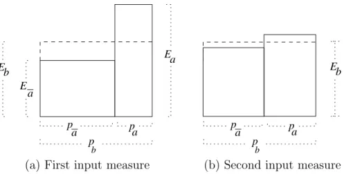
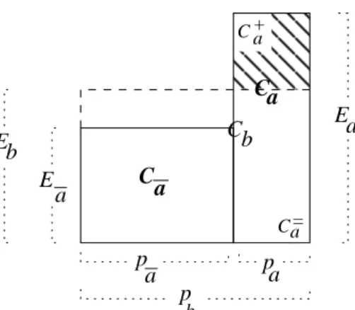
What are frequency bubble-deviations? Bubble deviation is a measure of the degree to which the collection of initial conditions departs from macroperiodicity. More specifically (Figure 3a):
The (absolute)bubble-deviation for
• a collection of inputs to a causal map device,
• a bubbleb, and
• an outcomeA,
is the absolute value of the difference between
• Ea, the (input-probability weighted) average number of inputs inbwhich lead to
outcomeA, and
• Eb, the overall average number of inputs inb,
divided by the input probabilitypb of the bubbleb:
absolute bubble-deviation of A−1 in b = Eb−Ea
pb
.
Thefrequency bubble-deviation is the absolute bubble deviation divided by the sizeN of the the collection of inputs:
frequency bubble-deviation of A−1 inb = 1 N Eb−Ea pb .
This is a sort of measure-theoretic analogue of the slope of a distribution of initial conditions, which does not require that the distribution be continuous, or even that the input space be defined by real-valued dimensions.
a E Ea p a a p Eb p b b a p p a b p E
(a) First input measure (b) Second input measure
Figure 3: Initial condition distribution within a bubble. Width represents measure.
The microconstancy inequality theorem implies that when bubble measures and bubble-deviations are small, outcome frequencies must be near to outcome probabilities. Note that for the sake of exposition, I use a number of vague descriptions informally in various parts of the paper (e.g. “a
large number ofsmall bubbles”). However, much of the vagueness is made irrelevant in the end by the fact that the inequality theorem makes precise the degree to which bubble measure and other quantities constrain frequencies to be near probabilities.
The microconstancy inequality theorem is similar to Strevens’ (2003, 2.3, p. 136) central the-orem on microconstancy, but has some advantages over it. Strevens’ thethe-orem doesn’t support a mathematical specification of the degree to which frequencies must be near probabilities. More importantly, unlike Strevens’ theorem, the inequality theorem doesn’t depend on an assumption that the input space is defined by real-valued dimensions. This allows FFF mechanistic probability to apply when the input space doesn’t lend itself to real-valued dimensions, and avoids any need to provide a naturalistic justification of choices of units for real-valued dimensions (cf. §§4.1, 5.2 below).17
The appendix presents the theorem more carefully and proves it.
3.2
Adjusting input measures
Now, some input distributions will generate small bubble-deviations relative to a given input mea-sure. A different set of input distributions might each generate large deviations. However, the latter distributions could nevertheless generate small deviations relative to a different input mea-sure. For example, some distributions will have large bubble-deviations relative to a particular input measure partly because frequencies overa=A−1∩bare usually much larger than frequencies overa=A−1∩b. Such distributions would nevertheless get small bubble-deviations if we changed the input measure, increasingP(a|b) and reducing P(a|b) within each bubble b. In Figure 3, each 17Strevens does have a strategy for applying his approach to systems which are not defined by real-valued dimensions (Strevens, 2003,§2.42 and Ch. 4), but the strategy is complex and makes additional assumptions about the systems to which it is supposed to apply. On the other hand, the fact that Strevens’ theorem is explicitly defined in terms of distinct real-valued dimensions rather than an abstract measure, supports a framework which allows Strevens to derive some interesting and useful results (Strevens, 2003, especially Chs. 2, 3).
diagram represents the same number of inputs (area) in a as the other diagram does; likewise for a. However, each diagram represents a different input probability measure (width). Since both measures assign the same value to the bubble’s probability,pb, the they differ in outcome-inverses’
conditional probabilitiespa,pa. As a result, the bubble-deviation in the right-hand diagram is less
than that on the left.
3.3
Application to construction of an interpretation
As mentioned above (§2.3), one can arbitrarily define any number of input probability measures for a causal map device, and such input measures can induce a derived probability measure on outcomes. However, as we’ve seen, something more is needed; frequencies of outcomes should at the very least tend to be near probabilities of outcomes, and for a systematic reason.
Suppose that, although actual distributions of inputs to a particular, causal map device vary quite a bit (e.g. distributions of spins, dice tosses, etc., by different croupiers), there is a micro-constant input probability measure that makes all or most such distributions macroperiodic. That this can be done for some devices is not implausible. For if there are many bubbles, it’s possible for the maximum bubble measure to be small, and (as I’ll argue in Section 5.3), there will be a sense in which it’s easy for distributions to be macroperiodic. Then by the above theorem, frequencies would be near to the outcome probabilities which are induced by input probabilities. Thus we might be able to define a sense of objective probability for outcomes of a bubbly causal map device in terms of the following conditions:
1. The fact that there’s a bubble partition and microconstant measure P on the input space which determine a small maximum bubble size.
2. Whatever facts make it the case that input distributions will have small bubble-deviations relative to this bubble partition and measure.
Outcome probabilities defined by that input measure will then be close to frequencies of outcomes resulting from such distributions. This is the intuition behind what I callmechanistic probability.18
The probability defined by conditions 1 and 2 will be a kind of objective probability as long as condition 2 involves only objective properties. Note that bubbliness is implied by condition 1, and makes it easier for condition 2 to be satisfied (§5.3).
At this point, we need a general method for constructing an input measure that allows the strategy to work (since we can’t, for example, simply assume that Lebesgue measure will do the job).19
4
Justification of an input measure
In this part of the paper I’ll present a naturalistic method for defining an input measure in terms of what I call “far flung frequencies” (FFF), which will satisfy something like conditions (1) and (2) above. This will allow us to define “FFF mechanistic probability” in terms of this input measure. 18In my terms, Streven’s (2011)’s “microconstant probability” and Rosenthal’s (2010) “natural range conception of probability” are varieties of mechanistic probability.
19One way of justifying the input measure would be to define it by the outcome measure of a causal map device which generates inputs to the present causal map device. But what explains that latter causal map device’s input measure (cf. (Strevens, 2003, Ch. 2))?
The inequality theorem will then imply that frequencies of an outcome will usually be near to the outcome’s FFF mechanistic probability. I’ll argue that FFF mechanistic probability has many of the properties that we should want in an objective interpretation of probability. (The strategy below, which is roughly to choose an input measure that allows the inequality theorem to have desirable implications, is analogous to defining a class of semantical models in terms of a set of axioms which they satisfy.)
I first consider and reject a way of defining an input measure proposed by Strevens for his microconstant probability interpretation, which is similar to FFF mechanistic probability (§4.1). I then define my notion of a “natural collection of inputs” (§4.2), and explain how an input probability measure can be defined by minimizing differences between probabilities and frequencies across all natural collections (§4.3). The resulting probability measure must succeed in in making most natural collections macroperiodic in order for FFF mechanistic probability to exist (§4.3). Later parts of the paper will clarify various aspects of the resulting notion of FFF mechanistic probability.
4.1
On Strevens’ input measure
Strevens (2011) describes an interpretation of probability—‘microconstant probability”—which is similar to FFF mechanistic probability in many respects. Strevens’ strategy is to define an input measure from the nomic character of the devices which generate inputs to a device such as a wheel of fortune. Here I briefly present an objection to Strevens’ way of defining an input measure. While I’m sympathetic to his strategy, at present I don’t see a way to make it work.
Strevens defines the input measurePas one which makes the actual inputs to a focal causal map device D macroperiodic, as long as these inputs are produced by a generating device (or devices) Gwhich has (have) a tendency to produce events which would be macroperiodic for Drelative to
P. We can’t, of course, require that this tendency be one which guarantees macroperiodic inputs; that would rule out streaks in which frequencies depart from probabilities. So Strevens says thatG has a “tendency” to produce such events just if it would produce events which are macroperiodic forD relative to P in “nearly all” of the closest possible worlds. However, as Strevens recognizes, this “nearly all” (e.g. 95%) requires a probability measure over the closest worlds. (We can’t just count closest worlds, since they seem to be uncountable (Lewis, 1973).) Note then, that Strevens’ characterization of the input-producing deviceG, and hence of the input measure and microconstant probability overall, depends fundamentally on providing a probability measure over certain possible worlds.
Strevens’ “nearly all” is defined by a Lebesgue measure specified by standard physical units, which characterize differences between physical processes involved in producing collections of inputs to D.20 But making the input measure depend on a probability defined by standard units seems arbitrary.21 Why standard units? Why is this the measure relevant to characterizing the proportion of closest worlds in which inputs are macroperiodic? Even if Lebesgue measure relative to standard units did work in some cases—for wheel of fortune croupiers, suppose—why expect that this strategy will generalize to other seemingly reasonable applications of microconstant/mechanistic probability? Even for the wheel of fortune, angular velocities produced by humans presumably depend on 20There is a perhaps minor lacuna in Strevens’ description of the measure over worlds, in that nothing is said about upper and lower bounds for the physical quantities; bounds would be needed to make the Lebesgue measure finite and normalized.
21Rosenthal’s (2010) “natural range conception of probability” also defines the input space in terms of standard units.
complex interactions between many neurons and other cells, responding to each other in various nonlinear ways. What reason is there to think that a measure defined in terms of underlying physical units for states of neurons will give large measure to counterfactual croupier states which produce macroperiodicity? Moreover, if we try to apply Strevens’ microconstant probability to cases in biological or social sciences, it becomes even less clear that standard units are relevant to defining a tendency of input-producers to give rise to macroperiodic distributions.
Thus I’m sceptical about the possibility of defining an input measure appropriate to mechanistic probability in terms of characteristics of input-producers. My strategy is instead to define the input measure directly in terms of certain sets of actual inputs produced by such devices. I’ll argue later that given the relationship of these set of inputs to bubbliness, FFF mechanistic probability will usually reflect the causal structure of input-producing devices to a significant degree.
4.2
Natural collections of inputs
Given a set of basic outcomes for a causal map device D which is bubbly with respect to those outcomes, we need a general way of specifying a probability measure on the device’s input space that can potentially produce an input measure that:
1. Is microconstant: The probability of each basic outcome-inverse should have the same value conditional on each bubble.
2. In some sense reflects patterns of inputs in the world in such a way that relevant collections of actual inputs to such devices tend to be macroperiodic, i.e. have small bubble-deviations. The idea here is that if we can define an input measure so that it reflects facts which are not just about inputs to the particular device of interest D (e.g. a particular wheel of fortune) but also to certain similar devices, we can capture general facts about such patterns of inputs in our world.
I’ll define the input measure for a causal map device D in terms of patterns of actual inputs to devices with roughly the same input space as D. These other devices need not map inputs to outcomes in the same way as D, however. I’ll propose that we define the input probabilities for a deviceDin some way which reflects patterns of inputs to all actual devices with roughly the same input space as D, over a large region of space and time surrounding the period ofD’s functioning which is of interest. For example, the input probabilities for an actual wheel of fortune W might depend partly on inputs to other actual wheels of fortune with similar input spaces—similar ranges of angular velocities—but with different-sized wedges, different numbers of wedge colors, etc.; as well as spins of roulette wheels (ignoring the tosses of little balls); and spins of wheels inside mechanical one-armed bandit slot machines.
I’ll define the input measure for a causal map device in terms of relative frequencies in sets of distinct “natural collections of inputs”:
Natural collection of inputs with respect to a causal map device D:
A natural collection forDis a large set of all and only those actual inputs produced by a single source deviceG to a particular causal map deviceD∗ during a single interval of time T∗, whereD∗ has the same input space asD.
The source deviceG, for example, might be a human croupier. The strategy below will be to define an input measure for a bubbly causal map deviceDin terms of “far flung frequencies”: frequencies in a large set of all and only those natural collections of inputs to actual devicesD∗ (similar toD at least in having the same input space) within a large spatiotemporal region aroundD. Call this
an “a set of far flung (FF) natural collections of inputs”. I’ll explain shortly why the vagueness of this specification of relevant natural collections needn’t be problematic.
Note that the definition of “natural collection” is designed to rule out certain problematic cases. The fact that a natural collection must includeall inputs during an intervalT means that a collection can’t be restricted to inputs which produce a particular outcome (e.g. red). The definition also rules out natural collections which are the union of inputs from several input-producing devices (e.g. different croupiers). This allows us to distinguish between the actual world, in which outcome frequencies for wheels of fortune, roulette wheels, etc., are often close to probabilities, and a “robot croupier” world in which each croupier’s spins are restricted to a narrow velocity interval. Allowing unions of croupiers’ inputs to count as natural collections would mean that a group of robot croupiers with different narrow velocity distributions could define a natural collection, even though for any croupier in any period of time, outcomes would have more to do with the croupier than with the structure of a wheel of fortune.22
4.3
Constructing the input measure
Given a set of FF natural collections of inputs, we can define the input space of a bubbly causal map deviceDby choosing an input probability measure that minimizes differences between frequencies and probabilities across all natural collections in the set. More precisely, we should to choose measures for bubbles and for outcome-inverses which minimize the sum of squares of bubble-deviations for all of natural collections in the set.23 Since, according to the inequality theorem, bubble-deviations place a limit on how far outcome probabilities can be from frequencies, adjusting input probabilities to minimize bubble-deviations over the FF natural collections is a way to make outcome probabilities close to outcome frequencies in as many natural collections as possible.
Additional notation will be useful: Letcindex natural collections, bindex thenbubbles, anda index outcome-inverses for thembasic outcomes. Letpb be the input probability of bubbleb. Since
the input measure that we construct should be microconstant, we require that the probabilityqa=
pa/pb of outcome-inverse abe the same conditional on every bubble. Ecba will be the
probability-weighted average number of inputs from natural collectioncwithin outcome-inverseain bubbleb, whileEcbwill be the corresponding average over an entire bubble. LettingCcbrepresent the number
of inputs from natural collection c falling in bubbleb, and Ccba, the number of inputs also falling
in outcome-inversea, the bubble-deviation forain bubblebwith respect to natural collectioncis: Ecb−Ecba pb = Ccb pb − Ccba qapb pb = Ccb p2 b −Ccba qap2b .
22It might be possible to allow combinations of inputs from different sources or different intervals when the combinations are not too distant (e.g. all red vs. all black) by specifying a metric over collections of inputs (Christopher Hitchcock, pesonal communication).
23Minimizing a sum of squares is minimizing with respect to a natural metric: Viewing bubble-deviations as a distances along dimensions of a Euclidean space, the square root of the sum of squares is a common generalization of the Pythagorean theorem, and varies monotonically with its square. That FFF mechanistic probability constructs a measure by minimizing a sum of squares involving actual frequencies is reminiscent of Gilboa et al.’s (2010) interpretation of probability. However, Gilboa et al.’s interpretation has different goals, is defined in terms of a different set of actual frequencies, and does not make use of anything like bubbly causal structure.
The quantity to be minimized by adjusting the pb’s and qa’s is thus ∑ c ∑ b ∑ a ( Ecb−Ecba pb )2 = ∑ c,b,a ( Ccb p2b − Ccba qap2b )2 ,
This is a function of n variables pb and m variables qa, with
∑ pb and
∑
qa each constrained to
equal 1. The C’s, which are numbers of inputs falling in certain regions, are constants determined by the set of FF natural collections with respect to which we want minimize probability/frequency differences. Bubble-deviations in larger natural collections should have a greater influence on the input probabilities than those those in smaller collections. This is captured here by the fact that bubble-deviations use absolute rather than relative frequencies. Thus bubble-deviations in larger natural collections will put more inputs into each bubble and outcome-inverse on average, with correspondingly larger bubble-deviations. Whether some other weighting of natural collections makes more sense is a question for future research.24
I don’t claim that it’s straightforward to minimize the above function analytically, although numerical approximation might be practical if data on all relevant natural collections were available. Section 5.5 discusses further issues concerning the epistemology of FFF mechanistic probability.
Nothing I’ve said implies that the input measure defined by the above minimization will actually produce small bubble-deviations (i.e. macroperiodicity) for most of the FF natural collections. If the natural collections vary too wildly, even minimum bubble-deviations will be large. That would mean that the processes which produce inputs to such devices are simply too varied in their effects to produce stable relative frequencies (even for a device bubbly with respect to the constructed input measure). In such a case we may seem to have some of the ingredients for mechanistic probability, but the best possible input measure isn’t good enough; FFF mechanistic probability simply doesn’t exist here. (Cutoffs for the definition of FFF mechanistic probability could be specified if desired; e.g. we could require that maximum bubble deviation be no more than .05 in at least 95% of natural collections.)
5
FFF mechanistic probability
Here I’ll pull together the aspects of FFF mechanistic probability outlined above and discuss con-sequences and potential problems of the resulting interpretation.
5.1
Summary of the interpretation
FFF Mechanistic probability exists for a particular actual causal map device D and a specified partition of its output space into basic outcomes only if:
1. There is a large set of FF natural collections of inputs—i.e. a set containing all and only those collections of inputs to actual devices D∗ such that
(a) The inputs are all and only those produced by a single physical device;
24I don’t assume that there’s a single global minimum, but since bubble-deviations constrain outcome frequencies to be generally close to outcome probabilities, any set ofpb’s andqa’s which give rise to the same
(b) D∗ has approximately the same input space as D;25
(c) D∗ occurs within a large spatiotemporal region around the location and time ofD; 2. (a) Dis bubbly: A bubble partition forDwith a large number of bubbles exists, such that:
(b) A microconstant input measure, constructed through minimization of the sum of squares of bubble-deviations for all members of the set of FF natural collections, makes most of the collections macroperiodic relative to this input space and the device’s bubble partition. (Or: Most collections generate a small maximum bubble-deviation.)
The mechanistic probability of an outcome A is then the input probability of its overall outcome-inverse A−1: the probability of all inputs which can cause A by the operation of the causal map device. The inequality theorem specifies how close frequencies will usually be to probabilities.
This proposal is preliminary, and has rough edges, some of which I’ll discuss below. One apparent problem is the vagueness of “broad spatiotemporal region” around D, which defines the set of FF natural collections. This problem can be mitigated by adding the following requirement to those above:
2. (c) Moderately expanding or contracting the spatial or temporal range across which nat-ural collections are defined doesn’t affect whether condition 2b is met, and doesn’t significantly change the probabilities of outcomes.
The idea is that if a significant change in outcome probabilities results from expanding or con-tracting the “far flung” region over which the set of natural collections is defined, then there’s something special about input frequencies in some regions rather than others, and these differences are primary determinants of outcome frequencies. In that case, it makes little sense to define an interpretation of probability in terms of bubbly causal structure of D (relative to an underlying pattern of frequencies—see below).
In summary, my proposal is that FFF mechanistic probability exists for the outcomes of a causal map device D if and only if requirements (1) and (2) are satisfied. Note that these re-quirements speak in vague terms of a “large number of bubbles”, and “small maximum bubble deviation”. However, since the microconstancy inequality theorem specifies a precise relationship between bubble measure (constrained by number of bubbles), bubble-deviation, and the difference between frequency and probability, choosing precise cutoffs for these values to define FFF mech-anistic probability isn’t essential. One could define a more precise version of FFF mechmech-anistic probability by specifying how close frequencies should be to probabilities, if desired.
5.2
Bubbles relative to natural collections
It might be argued that bubbliness can’t play any special role in distinguishing FFF mechanistic probability from an actual frequency interpretation of probability which averages over natural collections. For there’s a sense in which nearly every causal map device is bubbly. Understanding why will help to motivate the phrasing of condition (2), clarify the character of FFF mechanistic probability, and show that it doesn’t require our earlier heuristic assumption that input spaces are provided with metrics (§2.2).
25Perhaps the D∗’s should be required to be similar to D in other respects as well; this is an issue for future investigation (cf. (Strevens, 2011)).
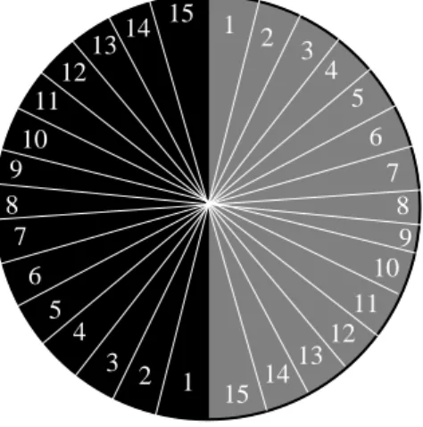
2 3 4 5 6 8 4 5 6 7 8 9 11 10 12 13 9 12 13 14 15 15 1 2 1 3 7 10 11 14
Figure 4: Each pair of regions numbered the same makes up a single bubble.
Consider thebig wheel, a heavy wheel of fortune of large diameter divided into two semicircular regions, colored red and black. Assume that the mass and friction of the wheel is such that many croupiers will primarily produce spins leading to a single outcome, either red or black, depending on the croupier’s strength. Intuitively, the big wheel doesn’t seem bubbly, since any given croupier’s spin distribution isn’t broken up into many bubbles leading to both red and black outcomes.
However, if we drop the temporary assumption of Section 2.2 that bubbles are contiguous, we can construct a bubble-partition in the following way: Starting from each end of the diameter separating the red and black regions, let the first bubble be composed of the wedge extending one centimeter along the wheel’s edge into the black region, and the wedge extending one centimeter from the other end into the red region (cf. Figure 4). The next bubble is similarly composed of wedges from the black and red regions extending one centimeter in each direction, and so on for all bubbles. Each bubble is composed of a slice of the black region and a slice of the red region, although slices within each bubble are not adjacent. We have thus partitioned the input space into many bubbles, i.e. subsets which contain points (velocities) leading to each outcome. The big wheel is thus bubbly, despite the intuition that it only has two semicircular “wedges”.26
Yet given what I’ve said about the wheel and its croupiers, if the wheel happened to produce stable frequencies, this would be due to the luck of the wheel being spun by a series of mainly strong or mainly weak croupiers. The big wheel’s causal structure plays little if any role in producing stability. Merely requiring a causal map device to be bubbly is to place no particular constraint on the causal structure of the device.
One solution is to place additional constraints on bubbles. Codifying the earlier assumption that all portions of a bubble are contiguous would rule out the big wheel as a bubbly device. For input spaces with at least two dimensions, we could also exclude bizarrely shaped bubbles which are continuous only because a slender thread in the input space connects otherwise discontinuous subsets. So far, though, I’ve only provided a naturalistic construction of a measure on the input space. Constraints on contiguity and shapes of bubbles would require, in addition, a naturalistic construction of a metric. (In a related context, Strevens (2003, Ch. 2) adopts a strategy of this kind, requiring bubbles to be contiguous and “reasonably compact” (p. 56), and using, for example, a Euclidean metric derived from real-valued physical quantities defining input space of a device.
However, this makes it difficult to apply FFF mechanistic probability to systems whose input spaces aren’t defined by real dimensions—e.g. the causal map device for flowering plants mentioned in Section 2.3.27)
However, condition (2) for FFF mechanistic probability avoids the need for a metric by requiring (2a) that a relevant bubble-partition must be one (2b) that allows the FF natural collections to determine an appropriate input measure. That is, (2) requires that the device be bubbly relative
to an input measure which satisfies the requirements of (2b). The fact that for some causal map devices, most natural collections are macroperiodic with respect to a single way of organizing the input space into bubbles seems to show that the bubble-partition captures something systematic about the world—something about the processes which generate the natural collections, perhaps.
I do think that in most obvious applications of FFF mechanistic probability, bubbles will be contiguous and compact in an intuitive sense. At various points earlier in this paper I partly depended on readers’ intuitions that this was so in order to simplify presentation. However, FFF mechanistic probability does not require that bubbles form neat contiguous sets in a Euclidean space, and there is no need to justify a metric on the input space. (References to bubbliness below should be understood as relative to an actual set of FF natural collections.)
5.3
Consequences of bubbliness
Bubbliness provides much of the warrant for other aspects of the concept of FFF mechanistic probability, including its dependence on natural collections of inputs.
It’s the bubbliness of a causal map device that buffers outcome frequencies from much of the variation in frequencies within the FF natural collections: Many different kinds of natural collections produce the same outcome frequencies, which are near to outcome probabilities. Similarly, many counterfactually different natural collections would produce the same outcome frequencies and probabilities as well. Nothing like this last claim can be made about a simple finite frequency interpretation of probability: Every counterfactual difference in frequency determines exactly the same difference in probability. Best System chances can have the same property, since chances are sometimes defined by precisely those values which frequencies happen to have. The following argument should clarify the sense in which FFF mechanistic probability buffers counterfactual frequency differences.28
Suppose that FFF mechanistic probability exists for a given causal map device Din the actual world. Thus most natural collections for D are macroperiodic relative to the input measure that results from minimization. Here are three classes of counterfactual scenarios concerning natural collections.
1. In the alternative world, there is an input measure relative to which most natural collections are macroperiodic, and the input measure gives outcomes the same mechanistic probabilities as in the actual world.
2. In the alternative world, there is an input measure relative to which most natural collections are macroperiodic, but it gives some outcomes different mechanistic probabilities than in the 27But cf. (Strevens, 2003,§2.42 and Ch. 4).
28The argument has similarities to arguments in statistical mechanics, e.g. in Boltzman’s explanation of the behavior of gasses (Ruhla, 1989; Sklar, 1993), and to Strevens’ “perturbation argument” (Strevens, 2003, §2.53). However, those arguments depend on physical assumptions and attempt to justify stronger conclusions.
actual world.
3. In the alternative world, there is no input measure which makes most natural collections in the alternative world macroperiodic. Mechanistic probability for D doesn’t exist in the alternative world.
Let us say that worlds in class 1 “preserve” the FFF mechanistic probability that exists in the actual world, while worlds in classes (2) and (3) “break” it.
I claim that a consequence of the way that FFF mechanistic probability is defined in terms of bubbliness is that there is a natural sense in which there are more ways to preserve FFF mechanistic probability than to break it. Here I am individuating “ways” to produce counterfactual scenarios not by any metrical difference such as a difference in physical values between worlds, but simply by how many inputs must be counterfactually transferred between one bubble and/or outcome-inverse to turn an actual natural collection into a counterfactual counterpart of the same size. (Similar reasoning can be used to define ways involving counterfactual additions or deletions of inputs.) Note that finer-grained differences between natural collections don’t make a difference to FFF mechanistic probability. There are other strategies for classifying counterfactual differences between natural collections, but I’ll argue below that the one used here is most often appropriate to understanding FFF mechanistic probability.
There are many ways to counterfactually preserve FFF mechanistic probability. As long as natural collections are large enough, moving one, or two, or any small number of inputs from any bubble to any other within a natural collection would not significantly change bubble-deviations relative to the actual-world input measure. In general, FFF mechanistic probability is preserved if inputs are moved around within a natural collection in such a way that no bubble deviation is altered very much in any bubble, but with many bubbles and a large natural collection, there are many ways to do that. In fact, as long as there are are many natural collections, even counterfactually destroying the macroperiodicity of a single natural collection would not change the input measure, either. (Only most natural collections must be macroperiodic.)
By contrast, breaking FFF mechanistic probability requires that many inputs be moved to or from a few bubble/outcome-inverse combinations (“BO”s) (for class 3), or that many inputs be moved to or from the same outcome-inverse in many bubbles (class 2). But the number of ways of realizing scenarios 2 and 3 is constrained more by the number of bubbles and outcome inverses than by the size of a natural collection; for preservation, the reverse is true.
One can get a clearer sense of this difference in number of ways of preserving and breaking FFF mechanistic probability by looking more closely at some extreme cases. Suppose a bubble-partition hasnbubbles, and consider one outcome and its complement. For a single natural collection, there are 2n ways to interfere with macroperiodicity by transferring of all of the inputs in the natural collection to a single BO (there are 2n BOs). If this were to occur in many natural collections in the same alternative world, FFF mechanistic probability would not be defined for the given causal map device.
At the other extreme, the following procedure produces minimal bunching up of inputs in BOs: Shift an input from a BO to one of the 2n−1 other BOs. Then choose a BO which has neither given nor received an input; this will the source of the next gift of an input. There are 2n−2 such BOs, and 2n−3 BOs to which it can give an input, avoiding BOs which have already given or received a donation. Continue this procedure until all BOs have given or received a single input. There are (2n−1)! different ways of doing this—i.e. of pairing BOs so that each participates in exactly one end of a transfer of an input. This is the number of ways that an actual natural collection can be