Your AP Knows How You Move: Fine-grained Device Motion Recognition through WiFi

(1)

Your AP Knows How You Move:

Fine-grained Device Motion Recognition through WiFi

Yunze Zeng, Parth H. Pathak, Chao Xu, Prasant Mohapatra

Computer Science Department, University of California, Davis, CA, 95616, USA

Email: {zeng, phpathak, haxu, pmohapatra}@ucdavis.edu

ABSTRACT

Recent WiFi standards use Channel State Information (CSI) feedback for better MIMO and rate adaptation. CSI pro-vides detailed information about current channel conditions for different subcarriers and spatial streams. In this paper, we show that CSI feedback from a client to the AP can be used to recognize different fine-grained motions of the client. We find that CSI can not only identify if the client is in mo-tion or not, but also classify different types of momo-tions. To this end, we propose APsense, a framework that uses CSI to estimate the sensor patterns of the client. It is observed that client’s sensor (e.g. accelerometer) values are correlated to CSI values available at the AP. We show that using simple machine learning classifiers, APsense can classify different motions with accuracy as high as 90%.

Categories and Subject Descriptors

C.2.1 [Computer Systems Organization]: Network Ar-chitecture and Design—Wireless Communication

Keywords

APsense, Device Motion Recognition, Wireless Sensing, WiFi

1. INTRODUCTION

In this paper, we propose APsense, a framework using which an Access Point(AP) can estimate the patterns of mo-tion sensors of an associated smartphone. APsense, bringing the sensing capability to the AP, can classify fine-grained motion of the smartphone which is typically only available through Accelerometer, Magnetometer and Gyroscope (AMG) sensors. APsense can be implemented on off-the-shelf com-modity hardware without any additional communication over-head. In order to perform fine-grained device motion detec-tion, APsense uses CSI feedback information from the client smartphone and extracts useful features that are indicative of fine-grained motion. We show that changes in CSI feed-back at the AP has a strong correlation with how observed

Permission to make digital or hard copies of all or part of this work for personal or classroom use is granted without fee provided that copies are not made or distributed for profit or commercial advantage and that copies bear this notice and the full cita-tion on the first page. Copyrights for components of this work owned by others than ACM must be honored. Abstracting with credit is permitted. To copy otherwise, or re-publish, to post on servers or to redistribute to lists, requires prior specific permission and/or a fee. Request permissions from [email protected].

values of AMG sensors change on the smartphone. As CSI feedback is commonly being used in newer MIMO and MU-MIMO systems, predicting fine-grained motion using CSI does not require any additional communication. Estimating how AMG sensor pattern changes can be used for many dif-ferent applications such as gesture recognition and activity recognition (e.g. walking, running etc.).

The major contributions of our work are as follows:

•Identify Motion: First, we show that CSI feedback received at the AP from client smartphone can reflect fine-grained motion of the smartphone. We perform experiments on commodity NIC to collect CSI traces at different loca-tions and show that it can clearly distinguish between the cases where client is stationary or has fine-grained motion.

•Classify Different Motion Types:Next, we demon-strate that certain features extracted from CSI can create a unique signature for different types of motion. We evaluate this using four different types of motion (described in Sec-tion 3) and observe that CSI features can uniquely identify them with simple machine learning algorithms. Based on this, we design APsense framework which consists of ma-chine learning classifier that can learn and classify within a very short time period. Our evaluation shows that APsense can classify different motions with overall accuracy greater than 90% in certain cases.

•Correlate CSI and Sensor values:We then correlate the CSI feedback values to smartphone’s AMG sensors, and show that there exists a strong correlation between them. We think this is an important first step towards our ulti-mate goal which is to derive AMG sensor patterns using CSI feedback. Since there are plethora of applications de-signed on smartphone’s AMG sensors, deriving their values passively using CSI would be extremely useful. As a first step, we establish the correlation between them and leave the actual derivation to our ongoing work.

2. RELATED WORK

Sensing using the wireless signals has gained a lot of atten-tion recently. There are multiple characteristics of the signal that can be used for the purpose of sensing motion. RSSI, which measures the received radio signal power, has been used for the purpose in some of the recent work. Youssef et. al. [7] introduced a system that can detect and track a mov-ing object usmov-ing RSSI. More recently, Wang et. al. [4] pro-posed to use RSSI to predict the length of human queues in public areas. However, RSSI is a coarse-grained abstracted measure and can not be used for detecting fine-grained mo-tion. Compared to RSSI, CSI is a much more fine-grained measure of the wireless channel. Wu et. al. [5] leveraged

(2)

CSI to perform a more accurate indoor localization. Recent work such as [8] and [6] have used CSI although their work is mostly limited to detecting motion in surrounding and not applicable to fine-grained motion detection (e.g. hand gestures). Pu et. al. [3] designed a system that can recog-nize human gesture based on the doppler shift of the wireless signals although such system can not be implemented using off-the-shelf hardware.

All the above work mostly deal with device-free motion detection, while our focus is in this work is different. We are interested in detecting fine-grained motion of a client device (e.g. smartphone) when it is associated with an AP. Our objective is to build a sensing framework where AP can understand client’s sensor patterns purely using wireless sig-nals. We think that such a framework can enable a number of novel applications.

3. CSI AND MOTION

3.1 CSI Background

Current WiFi standards like 802.11n and 802.11ac use OFDM in their physical layer. OFDM divides the channel into multiple subcarriers and data is sent over the subcar-riers using the same modulation and coding scheme. This partitioning of the channel into subcarriers allows OFDM to combat the frequency selective fading due to multipath. Because each subcarrier is smaller than the coherence band-width, it suffers from independent flat fading. This way, the effect of multipath on different subcarriers can be considered more or less uncorrelated.

The CSI information represents signal strength and phase information for OFDM subcarriers. The received signal can be modeled as

y=H·x+n (1)

whereyis the received signal,xis the transmitted signal,n is the channel noise andH is the CSI which is a complex-number matrix that indicates the channel frequency response of each individual subcarrier for every spatial stream. This way, CSI for all subcarriers and all spatial streams is a m×n×w matrix, where m is the number of transmitter antennas,nis the number of receiver antennas andwis the number of subcarriers. Such a fine-grained matrix can accu-rately capture the temporal and spectral conditions of the channel and changes caused by small-scale multipath effects. Our proposed APsense framework is leveraging the afore-mentioned properties of CSI to recognize the fine grained motions of the receiver and further predict the sensor pat-terns of the receiver on the AP side.

Until recently, CSI values were not available outside the NIC firmware which made it difficult to use it for any other application. Recently, Harperin et. al. [2] developed firmware and driver support for Intel 5300 802.11n NIC that can ex-tract the CSI values in kernel/user space. We use their tool in our work. Note that although 802.11n utilizes 56 subcar-riers in a 20 MHz channel, the CSI tool [2] reports 30 values for 30 groups evenly spread over the 56 subcarriers. This way, CSI for one spatial stream is a vector

H= [H1, H2, . . . , H30] (2)

whereHi represents theith subcarrier group. Hiis a com-plex number representing both amplitude and phase responses

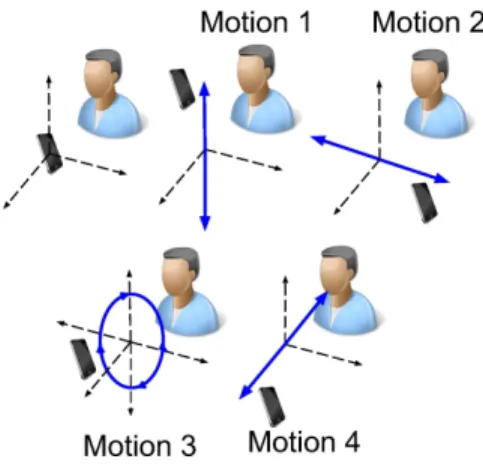
Figure 1: Different type of hand motions studied in APsense as follows

Hi=|h|ejp (3)

where|h|is the amplitude andpis the phase.

3.2 Experimental Settings

We use CSI tool [2] enabled on Intel 5300 802.11n NIC with three external antennas as the receiver to collect the CSI data which will be eventually available on the AP side through the feedback information. In order to understand the relationship between CSI changes and motion patterns, we attach a Shimmer [1] device at the center of the external antennas. The Shimmer device has accelerometer, magne-tometer and gyroscope sensors, and we collect their values to establish ground truth in our comparison. To check if CSI can classify motions or not, we try four separate hand move-ments as shown in Fig. 1. Albeit simple, these motions can be combined to generate many other complex gestures. In our experiments, the client stays at the same location, fac-ing towards the AP in a line-of-sight link. We repeat each motion 50 times while collecting both the CSI and Shimmer sensor data. The CSI is collected at a rate of 10 samples per second for a more tractable analysis, while the Shimmer data is collected at 100 samples per second for higher accuracy in understanding the motion type. The same experiments are repeated for a case where the client device is stationary in order to establish a base line for comparison. We also repeat the experiments at four different indoor locations. In order to reduce the impact of excessive multipath in our ex-periments, we perform the experiments at night time with nearly no movement of surrounding objects.

3.3 Identifying Motion Using CSI

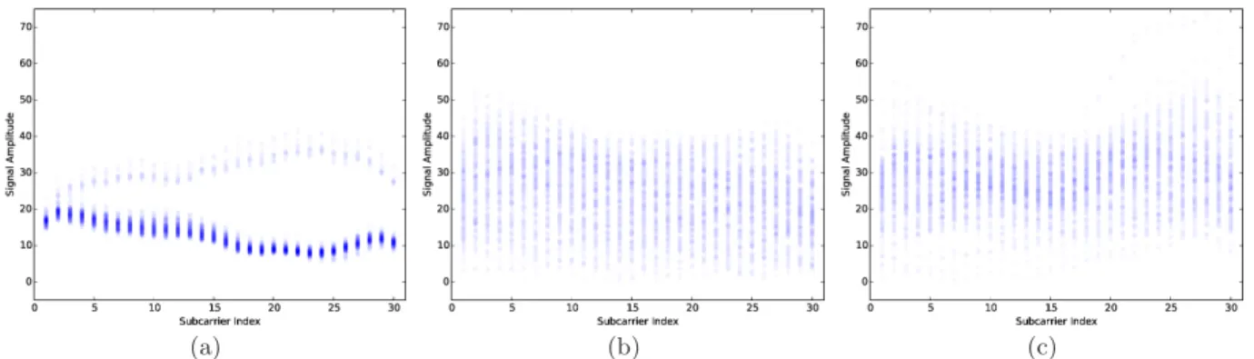
Now we take a look at how fine grained motions can affect CSI. Our observation is that the multipath changes due to small motion affect individual subcarriers and each subcar-rier suffers from uncorrelated flat fading. Also, we observe that different subcarriers are affected in different ways for different motions. To demonstrate this, we collect CSI traces for three cases - device is stationary, motion 1 and motion 2 (Fig. 1). Fig. 2 shows the observed CSI amplitude density distribution for each subcarrier within a 30 seconds’ trace. As we can see in Fig. 2a, in the case where there is no mo-tion, the amplitude values are much more concentrated. On the other hand, Figs. 2b and 2c shows that in the case of motion, the CSI amplitude is much more dispersed.

(3)

Com-(a) (b) (c)

Figure 2: Density Distribution of CSI amplitude in each subcarrier for a 30s trace where client is (a) stationary, (b) in motion 1 and (c) in motion 4. The x axis is the subcarrier index from 1 to 30 and the y axis is the CSI amplitude.

paring Fig. 2a with Figs. 2b and 2c shows that CSI can clearly identify if the device is stationary or in motion. Fur-thermore, the pattern of dispersion in Figs. 2b and 2c is noticeably different which tells us that a closer look at the CSI values can in fact classify different types of motions as well.

3.4 Classifying Motions using CSI

We now know that CSI can identify whether or not the receiver is in motion. Next, we take a step further to see if CSI can also be used to classify different types of motion.

3.4.1 How is CSI Influenced by Motion?

Before doing rigorous feature extraction, we first calculate some obvious yet important statistics about the subcarrier-level information available in CSI. We first divide the CSI data in time windows of t seconds and calculate different statistics for each time window. As an example, we calculate the mean of amplitude of 30 subcarriers at for all samples in a time window and find the 90th percentiles of the mean values. Intuitively, this should reflect the upper limit of mean values in the time window without considering the impact of outliers. As shown in Fig. 3a, the 90th percentile of mean values is noticeably different for different motion types. This is because different motion has different effect on the maximum amplitude of all subcarriers. Next, we take a look at a specific randomly chosen subcarrier and calculate the standard deviation of its amplitude values in given time window. As shown in Fig. 3b, we observe that this value can be used to distinguish between static case, motion 3 and motion 4. Note that although the same value can not be used for classifying motions 1 and 2, we see that the same statistic about other subcarriers can be used for that purpose. Next, we determine a more comprehensive set of features that we use for motion classification.

3.4.2 CSI Features Extraction

To find a more complete set of candidate features, we derive statistics in both time and frequency domains based on the raw CSI data. We use two sets of features - features for individual subcarrier and features across all subcarriers in a given time window.

Features for individual subcarrier: We calculate the following features using CSI amplitude value in each time window.

• Mean/Median - Measuring the static component of CSI amplitude with different motions’ impacts

• Min/Max/Range - Measuring the changing range of CSI amplitude

• Standard Deviation - Capturing the fluctuation level with in each time window

• Percentile at 10% / at 90% - Measuring the CSI am-plitude range without potential outliers.

• Normalized Energy - Capturing periodic changing pat-terns caused by different motion. Here, we use FFT to calculate the samples in frequency domain.

• Normalized Entropy - Measuring the degree of disorder using the frequency domain samples

Features across all subcarriers:To calculate a feature across all subcarriers, we first calculate its value for a specific CSI sample. We then take various statistics of that over the time window where there are many different CSI samples. For each feature calculated over all subcarriers, we calculate its mean, min, max, range, standard deviation, skewness and kurtosis over the time window.

In addition, to have a overall comparison in each time window, for each time windowT, we can get the following matrix across subcarriers

H_{= [H}₁T,H2T,HiT,· · ·,HTT] (4)

whereHiT is a vector of length 30 and includes the CSI

am-plitudes of all subcarriers forithtime sample. After calcu-lating the correlation matrix betweenHiT andHjT, we can

obtain the largest and the second largest normalized eigen-values as the other two features for CSI [6]. As described in [6], larger values of these two features indicate lesser or no motion. This can be seen in Figure. 3c which shows the largest eigenvalues of different motions.

Similarly, we also obtain the following matrix across time between individual subcarriers

S= [S1,S2,Si,· · ·,S30] (5)

whereSiis vector of lengthT and includes all the CSI

am-plitudes for ith subcarrier in this time window. We also get a correlation matrix by calculating the correlation be-tweenSiandSj. Then, we obtain the largest and the second

largest normalized eigenvalues of the correlation matrix and use them as the features for CSI.

(4)

(a) (b) (c) Figure 3: Comparison different CSI features for different types of motions

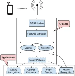
Figure 4: APsense Architecture

4. APSENSE

In this section, we introduce APsense, our framework that uses CSI feedback at the AP to recognize the fine-grained motion of the associated clients. As we mentioned before, the ultimate goal of APsense is to estimate the sensor read-ing patterns (e.g. accelerometer) of the clients. Such CSI-based sensing of client’s sensors on AP side can enable nu-merous new applications without requiring any additional message overhead. In this work, we have focused on classi-fying different motions as a first step towards it.

4.1 System Overview

The architecture of APsense is shown in Fig. 4. Here, the AP first collects the CSI information from the client smart-phone. It then extracts useful features from raw CSI data as shown in Section 3.4.2. These features are then used by ma-chine learning module that can learn and classify different motions. In the future, we plan to extend our system where machine learning module can recognize/classify sensor pat-terns (dotted boxes in Fig. 4) which can then be used for a number of different applications.

Machine Learning Model: To learn and classify dif-ferent motion based on CSI features, we use two commonly used supervised machine learning techniques -Naive Bayes

and Decision Tree. We choose these two methods because

the can handle non-linear nature of the features and their inter-dependencies. Also, decision tree can output simple if-else classification models that are useful in understanding the importance of different CSI features. We plan to use other more complex and customized classifiers in the future. Note that current design of APsense requires a small amount of client feedback for training the classifier. Here, the client device can provide the motion type to the AP along with the CSI data for some initial samples. Once the classifier model is built, it can then classify motions purely based on the CSI data.

4.2 Performance Evaluation

4.2.1 APsense at Different Locations

As explained in Section 3.2, we evaluate APsense at four different indoor locations. Table 1 shows the true positive rate of both machine learning methods for all four locations. Here, true positive rate is defined as the fraction of instances correctly classified as motion type X out of all instances ac-tually belonging to motion type X. As we can see, both the machine learning methods can very well classify different motions at all four locations. The classification accuracy is much higher (93.8% and 85.9%) for locations L1 and L3 because both the locations have much richer multipath envi-ronment compared to locations L2 and L4. We also combine instances of all the locations and perform a single classifi-cation across the loclassifi-cations. This is to evaluate how well our classification can work when the model is trained at a specific location. We observe in Table 1 that overall classi-fication accuracy drops (especially for Naive Bayes) in the combined case. This shows that APsense can achieve higher accuracy if the model is trained using location specific CSI profile.

Table 1: APsense Motion Recognition Results at Different Lo-cations - TP Rate

Method L1 L2 L3 L4 Combined

Naive Bayes 0.927 0.783 0.859 0.738 0.568 Decision Tree 0.938 0.774 0.815 0.786 0.748

(5)

L1 L2 L3 L4 Locations 0.0 0.2 0.4 0.6 0.8 1.0 TP R ate WIN = 2 sec WIN = 5 sec

Figure 5: TP Rate comparison with different time window sizes

Next, we take a look at the detailed results of combined locations case in Table 2. Here, precision is defined as ra-tio of number of true positives to the total number of true positive and false positives. The ROC (Receiver Operating Characteristics) area is the area under the curve when plot-ting FP rate versus TP rate. We can see that stationary case and motion 4 have a very high TP rate, while motions 1, 2 and 3 are often mis-classified reducing their TP rate. We believe that this is due to nature and directions of the motions. As shown in Fig. 1, motions 1, 2 and 3 are along the same X-Y plane, keeping the distance same from the AP. On the other hand, in motion 4, the motion is towards and away from the AP.

Table 2: Detailed Analysis for Combined Locations Case Motion Class TP Rate FP Rate Precision ROC Area

Static 0.989 0.007 0.978 0.997 Motion 1 0.592 0.079 0.646 0.892 Motion 2 0.614 0.072 0.672 0.920 Motion 3 0.625 0.098 0.580 0.891 Motion 4 0.848 0.054 0.778 0.969 Average 0.748 0.059 0.746 0.938

4.2.2 Time Window Size

The size of the time window over which we calculate the CSI features is an important factor. The above results are presented for the time window size of 5 seconds. We now ex-periment with changing the size of the time window to see its impact. Fig. 5 shows the comparison of TP rate for differ-ent locations with time window size of 2 and 5 seconds. We observe that larger time window size provides better classi-fication accuracy for all locations. This is mostly because more number of CSI samples are available for calculating features in the case of larger window size.

4.3 Correlating CSI and Sensor values

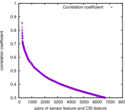
In our ongoing work, we plan to extend APsense such that it can estimate the client’s sensor pattern using the CSI data. To test the feasibility, we calculate different fea-tures of Shimmer sensor data collected in our experiments (Section 3.2). We then calculate one-on-one correlation of these features with CSI features. Intuitively, if these fea-tures are correlated to each other, it means that we can use the CSI data to derive how the sensor data changes. Fig. 6 shows the correlation coefficient for different pairs of CSI

0.3 0.4 0.5 0.6 0.7 0.8 0.9 1 0 1000 2000 3000 4000 5000 6000 7000 8000 correlation coefficient

pairs of sensor feature and CSI feature Correlation coefficient

Figure 6: Correlation between sensor and CSI features and sensor features. As we can see, a large number of pairs show a very high correlation which tells us that we can use the CSI features to derive the sensor patterns.

5. DISCUSSION AND CONCLUSION

In this work, we showed that CSI data can be used to determine client’s fine-grained motion at the AP. There are multiple challenges in APsense as it evolves in our ongo-ing work. First, it is expected that motion detection accu-racy would decrease when the surrounding environment has many moving objects and the resultant multipath is severe. Our current experiments were done in a controlled environ-ment with mostly stationary surroundings. We are address-ing these challenges as part of our ongoaddress-ing work. Second, since CSI samples are available only when actual frames are sent, it would become challenging to detect motion when available number of CSI samples are sparse. Revising the CSI features for fewer samples such that motion detection accuracy is still high is also an interesting direction of future work.

6. REFERENCES

[1] http://www.shimmersensing.com.

[2] D. Halperin, W. Hu, A. Sheth, and D. Wetherall. Tool release: Gathering 802.11n traces with channel state information.ACM SIGCOMM CCR, 41(1):53, Jan. 2011.

[3] Q. Pu, S. Gupta, S. Gollakota, and S. Patel.

Whole-home gesture recognition using wireless signals.

InProceedings of ACM Mobicom, 2013.

[4] Y. Wang, J. Yang, Y. Chen, H. Liu, M. Gruteser, and R. P. Martin. Tracking human queues using

single-point signal monitoring. InProceedings of ACM

MobiSys, 2014.

[5] K. Wu, J. Xiao, Y. Yi, D. Chen, X. Luo, and L. M. Ni. Csi-based indoor localization.IEEE Transactions on

Parallel and Distributed Systems, 24(7):1300–1309,

2013.

[6] J. Xiao, K. Wu, Y. Yi, L. Wang, and L. M. Ni. Fimd: Fine-grained device-free motion detection. In

Proceedings of IEEE ICPADS, 2012.

[7] M. Youssef, M. Mah, and A. Agrawala. Challenges: device-free passive localization for wireless

environments. InProceedings of ACM Mobicom, 2007. [8] Z. Zhou, Z. Yang, C. Wu, L. Shangguan, and Y. Liu.

Towards omnidirectional passive human detection. In