A Storage and Access Architecture for
Efficient Query Processing in Spatial Database Systems
Thomas Brinkhoff, Holger Horn, Hans-Peter Kriegel, Ralf SchneiderInstitute for Computer Science, University of Munich Leopoldstr. 11 B, W-8000 München 40, Germany
e-mail: {brink,holger,kriegel,ralf}@dbs.informatik.uni-muenchen.de
Abstract: Due to the high complexity of objects and queries and also due to extremely large data volumes, geographic database systems impose stringent requirements on their storage and access architecture with respect to efficient query processing. Performance improving concepts such as spatial storage and access structures, approximations, object decompositions and multi-phase query processing have been suggested and analyzed as single building blocks. In this paper, we describe a storage and access architecture which is composed from the above building blocks in a modular fashion. Additionally, we in-corporate into our architecture a new ingredient, the scene organization, for efficiently supporting set-oriented access of large-area region queries. An experimental performance comparison demonstrates that the concept of scene organization leads to considerable performance improvements for large-area region queries by a factor of up to 150.
1 Introduction
During the last decade, the management, representation and evaluation of spatial data in information systems gained increasing importance. Geographic information systems (GIS) are increasingly used in public administration, science and business. The nucleus of a GIS is the geographic database system. Contrary to business applications based on standard database systems, such systems are not suitable for geographic applications [Wid 91]. The insufficient expressive power e.g. of relational systems, leads to unnatu-ral data models and to poor efficiency in query processing.
Therefore, various research groups have developed a large number of concepts and techniques for improving single aspects of a geographic database system. Examples are the design of spatial data models or efficient access methods for managing large sets of spatial objects.
In this paper, we will present our geo architecture, a new storage and access archi-tecture for spatial objects integrating several concepts and techniques. It is not our goal to present a new spatial database system or a kernel of a system such as DASDBS [SW 86], EXODUS [CDRS 86], GRAL [Güt 89] and POSTGRES [SR 86]. Instead, we would like to assemble suitable concepts and techniques to a spatial query processing mechanism. One of the most important building blocks of our architecture is the scene organization, a new technique for supporting large range queries. Its performance im-provement by up to two orders of magnitude is demonstrated.
The paper is organized as follows. First, we take a closer look at the objects and op-erations commonly used in geographic information systems. This leads to a set of basic queries which should be efficiently supported by our architecture. A model of spatial query processing using different phases is described in section three. In section four, we present different algorithms and methods for supporting these phases. The new scene organization is described in section 4.4. The integration of the algorithms and methods
leads to our geo architecture. The rest of the paper contains an investigation of the per-formance of this architecture. In particular, we present a detailed perper-formance evalua-tion of our new scene organizaevalua-tion for real world data. The paper concludes with a brief statement of our findings and some suggestions for future work.
2 Objects and operations of a spatial database system
In this paper, we present a conceptional architecture for storing objects and processing queries in a geographic database system. To develop such an architecture, we first need an exact specification of the objects and queries. This is presented in the following sub-sections.
2.1 Objects
The objects stored in a geographic database are used for modeling specific parts of the surface of the earth with respect to one or several properties. Therefore, the objects are characterized by a spatial and a thematic component. The spatial component describes the spatial locality and the shape of the modeled part of reality whereas the thematic component contains the thematic information.
The spatial component
The spatial component of an object is represented by one of the basic topological ele-ments of the plane: point, line or area. Points are described by specifying their coordi-nates with respect to a given coordinate system. For modeling lines, both polylines as well as free-form curves are used. In this paper, we concentrate on representing areas. From the literature two main concepts for representing areas are known: the raster and the vector model. Because of its favorable scaling capabilities, its lower demand of stor-age and its “object orientation”, the vector model has been preferred over the last few years for application in geographic database systems. The type of spatial objects we consider in this paper is the class of simple polygons with holes (SPH for short) (see figure 1). A polygon is called simple if there is no pair of nonconsecutive edges sharing a point. A SPH is a simple polygon where simple polygonal holes may be cut out. The class of SPHs is well suited for geographic applications (see [Bur 86]). It allows repre-senting areas with arbitrary precision and explicitly takes holes into account.
Fig. 1. Simple polygon with holes The thematic component
The thematic component characterizes an object with respect to one or several thematic properties. We distinguish between qualitative properties such as land use and quanti-tative properties such as amount of precipitation. For representing thematic values, sim-ple data types such as strings or real numbers are used.
The object model
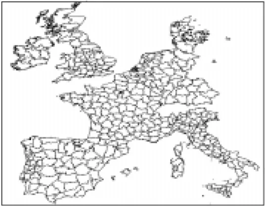
The geo architecture to be developed should be able to store sets of objects consisting of a spatial (SPH) and a thematic component (vector of simple data types). Figure 2 gives a typical example of a map which is represented by a set of SPHs.
Fig. 2. Map of the European counties modeled by a set of SPH
Both components require a completely different handling by the geo architecture. For managing vectors of simple data types, e.g. in a relational database system, a lot of well known data structures and algorithms are available. However, organizing the spatial component demands for new structures and algorithms. They should organize the ob-jects in such a way that spatial queries referring to location and shape of the obob-jects are processed efficiently.
Additional to these fundamental properties of the spatial objects, two more aspects are important for the design of the geo architecture. First, we need a characterization of the objects from real applications as accurate as possible. Second, we need a specifica-tion of the queries and operaspecifica-tions to be performed on these objects.
2.2 Characteristics of the objects
In this paper, it is not our goal to present a general characterization of the object sets occurring in geographic applications. From our point of view this is impossible because of the very wide application spectrum geographical information systems are used in. In-stead, we outline some general properties of the data which influence the design of our geo architecture considerably.
Complexity and variation of the data • Number of objects and data volume
In real applications, the number of data objects may be as high as 109. The data vol-ume may occupy up to 1 TerraByte (see [Fra 91] and [Cra 90]).
• Variation of objects and sets of objects
Data from real world applications vary extremely with respect to single objects and whole object sets [Fra 91]. This particularly refers to the following aspects: • Object extensions
It varies in a range of 1 : 106 [Fra 91], where the largest objects may occupy the whole data space.
• Object shape • Amount of storage
As an example, in the World Data Bank II [GC 87] the amount of storage for one polygonal object varies between 0.5 KB and more than 1.1 GB.
• Distribution of the objects in the data space
The number of objects per unit (density) varies in a range of 1 : 104 in real world applications [Fra 91].
In particular, we have to consider that there are no upper bounds neither for the exten-sion of objects, the complexity of object structure, the amount of storage, nor for the density of the objects.
Persistent storage of the objects in a weak dynamic environment
Recording the data of a geographic information system is an expensive task. Very often, data from paper maps as well as satellite pictures have to be integrated into a seamless database. This work is often a source of inaccuracy and inconsistency, which has to be revealed and removed by using time consuming consistency check mechanisms. Alto-gether recording the data and preserving consistency of the data account for approxi-mately 80% of the operating costs of a geographic database system [Aro 91].
After recording the database, it is persistently stored and used on a long term basis. However, the database is not static because correcting mistakes, removing inconsisten-cies and adapting to changes in the real world leads to updates of the data. All in all, the database is weakly dynamic.
The properties of spatial objects mentioned above and the queries and operations de-scribed in the following section form a requirement definition for the geo architecture which is described in detail in section 4.
2.3 Queries and operations
Geographic database systems are used in very different application environments. Therefore, it is not possible to find a compact set of spatial queries and operations ful-filling all requirements of geographic applications [SV 89]. Instead, we present four ba-sic classes of operations each with a number of typical representatives which should be supported by our architecture.
1) Modifications
Analogously to standard database systems, there are operations for insertion, deletion and update of records in a geographic database system.
2) Selections
We can distinguish between two types of selections: those referring to the spatial and those referring to the thematic component of an object.
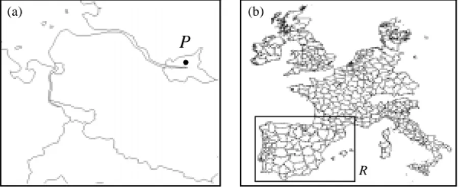
a) Spatial selections: • Point Query
Given a query point P and a set of objects M. The point query yields all the ob-jects of M geometrically containing P (see figure 3(a)).
• Region Query
Given a polygonal query region R (of type SPH) and a set of objects M, the re-gion query yields all the objects of M sharing points with R. A special case of the region query is the window query. The query region of a window query is given by a rectilinear rectangle (see figure 3(b)). Both, the window query and the re-gion query are often called range queries.
Fig. 3. Examples for a point and a window query b) Thematic Selections:
When performing a thematic (relational) selection the objects are selected with re-spect to properties of their thematic component. Within this section, we pay atten-tion only to the spatial component of the objects. In secatten-tion 4.5 we will describe how to support thematic selections.
3) Combinations • Spatial Join
For two given object sets A and B the spatial join operation yields all pairs of objects whose spatial components intersect. More precisely, for each object we have to look for all objects in B intersecting with a. Note, that for efficient processing of the spatial join a selective spatial access to the objects is nec-essary.
• Map Overlay
The map overlay is one of the most important operations in a geographic informa-tion system [Bur 86]. It combines two or more sets of spatial objects. This combi-nation is controlled by the overlay function determining in which way intersecting objects have to be handled. The map overlay is completely based on variants of the spatial join operation. In addition to the spatial join, the intersection of a pair of overlapping objects has to be computed. Neighboring objects with identical values of their thematic component should be merged [KBS 91].
4) Analyzing sets of objects
Selections or combinations of existing sets of objects are often followed by further processing steps in practical applications. The operations and algorithms used for these steps are very specific for a particular application and, therefore, are not supported by a general storage and access architecture. Without considering the details, we can distin-guish two classes of these operations and algorithms.
• Automatic analysis
Analyzing functions applied to the spatial and/or the thematic component of the ob-jects are part of this class. Typical representatives are: calculating the average of the area or perimeter of a set of objects, calculating the minimum and maximum of the-matic attributes etc.
• Visualization
In many cases the automatic analysis of a database is not possible and manual
inter-P
(a) R (b) a b, ( ),a∈A b, ∈B a∈Amediate steps performed by a user are necessary to complete the analysis. For this purpose, a visualization of the data on a graphic device is necessary.
The above mentioned facts clearly demonstrate that spatial selections are of great im-portance within the set of spatial queries and operations. They do not only represent an own query class, but also serve as a very important basis for the operations of the classes 2 - 4. Therefore, an efficient implementation of spatial selections is an important re-quirement for good performance of the complete geographic information system.
3 A phase model for geometric query processing
After the description and specification of objects and queries, we will design an archi-tecture for storing spatial objects and efficiently processing queries. The main task of the architecture is the efficient processing of spatial queries and operations. Therefore, in this section, we take a closer look at this type of queries, distinguish different phases in their processing and specify algorithms and data structures for their processing.
As mentioned in the last section, spatial selections are the most important basic op-eration in spatial query processing. Their execution can be described abstractly as a se-quence of steps:
Step 1: Scaling down the data space
Considering spatial selections in more detail, it turns out that only a local part of the complete data space has to be investigated. Only this area contains candidate objects that may fulfill a selective query.
For an efficient scaling down of the data space, it is essential to use data structures organizing the objects with respect to their spatial locality and shape. Obviously, ob-jects jointly fulfilling a query condition lie close together in the data space. Therefore, a physical clustering of the objects with respect to their spatial locality and shape is es-sential for providing efficient spatial query processing.
Due to the arbitrary complexity of real geographic objects, it is not possible to build up an index considering the complete information on the extension of the objects. Thus, the access method is not able to yield the exact result of a query. Instead, it excludes a large subset of objects from the result. A set of candidate objects that may fulfill the query condition remains and has to be passed on to step 2 of the query processing mech-anism. Orenstein established in [Ore 89] the terms filtering and refinement for this type of query processing.
Step 2: Exact investigation of the objects
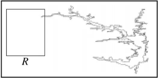
Step 2 of the query processing tests whether a candidate object actually fulfills the query condition or not. For that purpose, a spatial predicate, e.g. “polygon contains point” or “rectangle intersects polygon”, has to be checked. Similar to step 1, this test consists of different phases. First, the test has to be restricted to only that part of the object that is really relevant for the test. Figure 4 gives an example: To evaluate whether the query window R overlaps Lake Volta, only its northern west peak has to be examined.
Due to the complexity of the objects on the one hand and the selectivity of spatial queries on the other hand, it is useful to structure the objects locally. The resulting struc-ture elements have to be organized in a data strucstruc-ture referring to their spatial locality and extension. Using this data structure, we can efficiently decide which parts of the ob-ject are actually relevant to the query. Only this small number of local parts is further
examined using computational geometry algorithms, which finally decide whether an object fulfills the query or not.
Fig. 4. Test of a query window against Lake Volta Step 3: Output of objects for further processing
After identifying an object as part of the result, it is usually passed on to further process-ing e.g. analyzprocess-ing steps, output operations etc. Therefore, a physically connected stor-age of all parts of the objects is necessary to support a fast access to the complete object.
4 An architecture for query processing in spatial database systems
After the abstract description of the phase model for spatial query processing, we present algorithmic techniques for supporting the individual phases. Later on in this section, these techniques are used as building blocks within our geo architecture. 4.1 Spatial access methodsAccess methods as an essential part of the internal level of a database system are used to organize a dynamic set of objects on secondary storage. One-dimensional access methods like B-trees or linear hashing are not suitable for spatial database systems. For these systems, we have to look for data structures which organize the polygonal objects with respect to their location and extension in the data space. The arbitrary complexity of the spatial objects (simple polygon with holes) makes it very difficult to develop a structure considering the whole object description. Instead, we consider access methods for simpler two-dimensional objects. Surveys of spatial access methods can be found e.g. in [Sam 90] and [Wid 91].
Fig. 5. Schematic presentation of an R*-tree
The simplest class of two-dimensional objects are rectilinear rectangles. For this class of objects, a number of index structures already exists. A popular representative is the R-tree [Gut 84]. The R-tree stores as many spatially close objects (rectangles) on one data page as it accommodates and surrounds them by their minimum bounding box. A
R
directory level 1
directory level 2
set of such bounding boxes is stored on a (directory) page. Again, their minimum bounding box is computed and stored in a directory page one level above and so on. In this way, the whole object set is stepwise spatially clustered and a tree-like directory is created (see figure 5).
A very efficient version of the R-tree is the R*-tree [BKSS 90]. Within this data structure sophisticated algorithms for page splitting and local reorganizations are used. The overlap of page regions and the length of their margin are minimized as well as the dead space, i.e. the space occupied unnecessarily by page regions.
This idea of organizing rectangles leads to an efficient processing of point queries and small window queries [BKSS 90]. Unfortunately, this is restricted to rectangles or other simple spatial objects, not larger than a data page. In real applications, it is abso-lutely necessary to store more complex objects and to process large window queries ef-ficiently. Later on in this section, we will present an access architecture for managing arbitrary simple polygons with holes and processing large window queries efficiently. 4.2 Approximations
The set of results to a spatial query consists of all the objects fulfilling a geometric pred-icate e.g. containing a query point. As mentioned in the last section, spatial access meth-ods are used for excluding a large subset of the objects from the result as early as pos-sible. The remaining candidate objects have to be investigated by computational geom-etry algorithms. Considering complex objects (polygons with large numbers of vertices), this is a time consuming task. This leads to the idea of a geometric pretest. Such a test should be easy to process and should decide for a large number of objects whether they fulfill the query condition or not.
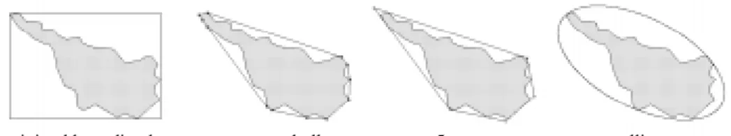
For implementing the idea of a geometric pretest, the concept of object approxima-tions is an adequate approach. In [Kri 91a] a detailed classification of different approx-imation techniques is given. The description of an approxapprox-imation should be simple and its quality should be high, two obviously competing criteria. To make object approxi-mations useful for a geometric pretest, the object has to be contained completely in its approximation (conservative approximation) [Sch 92]. Examples for conservative ap-proximations are minimal bounding boxes, convex polygons, ellipses etc. (figure 6).
Fig. 6. Various conservative approximations
Let us have a closer look at the processing of a point query using object approximations. First, for all candidate objects it is tested, whether their approximation contains the query point or not. In case of a negative result, the object does not contain the query point either. The object is discarded and a time consuming point-in-polygon test could be saved. Only in case of a positive pretest, the object itself has to be tested.
[BKS 93a] contains a detailed examination of object approximations used for spatial query processing in a real data environment. It turned out that the convex 5-corner is the best compromise between the approximation quality and storage amount. Using the
R*-tree, it is shown that other approximations than the minimal bounding box can effi-ciently be organized in a spatial access method originally designed for bounding boxes. 4.3 Object decompositions
Object approximations are applied to avoid complex geometric tests. Object decompo-sition techniques, however, are used to simplify and speed up their processing.
Consider again a point-in-polygon test. For processing this test an algorithm with linear runtime complexity is necessary [PS 88]. This examination of complex polygons i.e. polygons with thousands of vertices consumes a considerable amount of CPU time. On the other hand, only a small local part of the object is actually relevant for the deci-sion whether an object contains a point or not. This leads to the idea of object decom-position. Applying this idea, the objects are divided into a number of simple and local components, e.g. triangles, convex polygons etc.. During spatial query processing, only one or a small number of these components has to be checked. In [KHS 91] and [Kri 91a] the decomposition approach for simple polygons with holes is presented and discussed in detail.
Fig. 7. Three decomposition techniques for simple polygons
Using object decompositions geometric tests are applied only to components, e.g. trap-ezoids, which is much more efficient than testing the whole polygon. To decide which components are relevant for a particular test, we use again an R*-tree to organize the components of one object with respect to their location and shape. The resulting tree is called a TR*-tree. In [SK 91] we demonstrated that the TR*-tree efficiently supports various types of spatial queries and operations.
4.4 Scene organization
One important requirement for geographic database systems is the set orientation [Wid 91]. A spatial query processor has to perform small queries as well as large que-ries efficiently. When processing a large query, a large amount of data is transferred from secondary storage into main memory. The concepts presented up to now in this paper, merely support an efficient processing of small queries but do not speed up large queries considerably. Therefore, there is an obvious demand for a concept supporting set orientation.
Considering the existing storage organization and the type of objects to be stored, we can observe the following points:
• The objects are very large in comparison to the size of the pages they are stored in. Even in the case of large pages (e.g. 4 KByte), the number of objects per page is usu-ally small and often we need several pages for storing just one single object. • The pages used for storing objects are distributed on the secondary storage device
independently from spatial aspects, i.e. pages lying adjacent in space lose their neighborhood on the storage device. Large region queries transfer a large amount of
spatially adjacent pages into main memory. Therefore, an arbitrary distribution of these pages on the disk leads to very high access costs during query processing. The concepts presented in the sections before preserve only a local ordering within the pages [Wid 91]. To support the set orientation in an appropriate way, a global order preservation i.e. a physical clustering of larger storage units, is required.
Different approaches are conceivable to handle larger storage units. In [Wei 89] us-ing larger pages, pages of variable length, various bufferus-ing strategies and physical clustering of pages combined with a set-oriented interface are discussed in detail to han-dle large complex objects. In this paper, physical clustering of pages is favored and nat-urally offers itself as an adequate approach to store scenes within our geo architecture. To translate this approach into action, we need a set-oriented interface between the da-tabase system and the secondary storage device [Wei 89]. Such an interface allows an efficient transfer of physically adjacent pages from secondary storage to main memory. The implementation of such an interface is not the subject of this paper.
In [HSW 88] an idea based on dynamic z-hashing for implementing physical clus-tering of pages is presented. This idea is applied to rectangles in [HWZ 91]. However, the global order is preserved only for approximations of objects. Furthermore, this hash approach is not applicable to access methods with an arbitrary space partitioning scheme. Therefore, we have developed a concept based on the partitioning scheme of the R*-tree.
Building up the scene organization
As mentioned before, we use the R*-tree as a major component of our geo architecture, due to its good performance and its robustness. The R*-tree uses a very efficient scheme for space partitioning neither clipping nor transforming the spatial objects. These facts lead to the idea of using the partitions i.e. subtrees of the R*-tree as basic units for phys-ical clustering. In the following, a scene is defined as a subtree of the R*-tree physphys-ically clustered on secondary storage. One scene consists of a large set of physically adjacent pages containing all corresponding objects. Using this approach, no additional data structure for handling scenes is necessary.
An object larger than one page is stored on several pages such that all of them are physically clustered within one scene. Thus, also the transfer of such a large object into main memory is supported by the scene organization (see step 3 of the phase model). Note that no order has to be preserved within each scene.
Fig. 8. Scene organization
In addition to a schematic structure of the scene organization, figure 8 presents the par-ticular scene organization for the counties of the European Community (see figure 1
(a) approximations (b) scenes R*-tree
Level of scene description
subtrees for the scenes physically clustered
also). The R*-tree contains the polygons representing the counties, their decomposition components and their approximations (figure 8 (a)). Figure 8 (b) depicts the partition-ing of the R*-tree on a higher directory level. The rectangles describe the scenes, the corresponding subtrees are physically clustered.
Query processing
Using our scene architecture, small queries as well as large queries are processed effi-ciently. Small queries are processed by single page accesses as described before. If a range query specifies a larger query region, all scenes intersecting the query region, i.e. subtrees of the R*-tree, are transferred into the main memory. For each scene just one search operation on secondary storage is necessary. Without a scene organization, we need one search operation for each page which is much more expensive. Unfortunately, a scene may contain a number of objects not fulfilling the query condition (false hits). Nevertheless, the false hits are also transferred into main memory. A relatively small number of false hits does not affect performance considerably, since the time needed for searching a page drastically exceeds the time for transferring a page [PH 90]. In ad-dition, the degree of intersection between the scene and the query region may be used as a measure to decide whether the scene is transferred completely or whether the query is answered without using the scene organization. A detailed performance evaluation of the scene organization is presented in section 5.1.
After transferring the scene into main memory, a query is processed as usual, i.e. us-ing approximations and decomposition techniques (see section 4.2 and section 4.3). A detailed algorithmic description of the dynamic organization of the scene architecture is presented in [Sch 92] and [BKS 93b]. Supplementing the presented query processing techniques by a scene organization allows an efficient query processing for queries of arbitrary size.
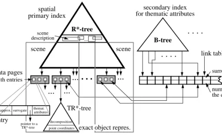
4.5 Integration of thematic attributes
The techniques presented up to now are completely dedicated to spatial queries. Que-ries referring to thematic attributes of the stored objects are also important in geographic information systems (see section 2.1).
For an efficient support of thematic queries, an additional index, i.e. a secondary in-dex (e.g. a B-tree) is necessary for the relevant thematic attributes. The R*-tree in co-operation with the scene organization determines the location of physical storage of the objects. For connecting both, we need a link table. This table assigns to each spatial ob-ject, which is represented by a unique surrogate one data page of the R*-tree. If the data page of the spatial object changes, only the entry of the link table has to be updated. An update of the secondary index is not necessary. To allow an access from the spatial in-dex to the link table, all entries of the spatial objects in the data pages have to be ex-tended by a surrogate.
In figure 9, the integration of a secondary index and a link table into our complete geo architecture is presented (for more details see also [Kri 91b] and [Sch 92]). 4.6 The geo architecture
Up to now, we have presented basic concepts and techniques for an efficient query processing in geographic databases. The goal of this section is the integration of these concepts into our geo architecture. This architecture is presented in figure 9.
The basic building block of our architecture is the R*-tree. It organizes the objects on secondary storage pagewise and allows an efficient spatial indexing. Starting with
the root, a spatial query passes through the R*-tree, thereby locating one or several scene descriptions. If the intersection of the query region and the scene exceeds a given threshold, the scene is completely transferred into main memory where query process-ing proceeds. Otherwise, the required data regions are transferred page by page.
The next ingredient of the architecture are approximations. They support a first preselection to determine whether an object fulfills the query or not. For that purpose, the approximations, e.g. minimal bounding 5-corners, of the objects are stored in the en-tries of the data pages. If the approximation of a spatial object fulfills the query, the ob-ject itself has to be further investigated. Therefore, each obob-ject entry contains a pointer to its exact geometric representation managed by a TR*-tree. The TR*-tree organizes all decomposition components and helps exploiting spatial selectivity in query process-ing. Instead of applying time consuming computational geometry algorithms to com-plete spatial objects, the query condition is evaluated just considering simple compo-nents.
The architecture is completed by secondary indices for thematic attributes. A the-matic query traverses the B-tree yielding one or more surrogates. These surrogates are used for accessing to the link table providing the number of the data page storing the object entry.
Fig. 9. Integration of efficient building blocks into our geo architecture
5 Evaluation
The techniques integrated in our architecture for spatial databases have been investi-gated and tested extensively. The basic component of the architecture is the R*-tree. In [BKSS 90] a detailed performance evaluation is presented and it turns out that the R*-tree outperforms the other R-tree variants. A performance comparison of the R*-tree, the R+-tree and the PMR-Quadtree is presented in [HS 92]. Various approxi-mations are compared in [BKS 93a]. The minimum bounding 5-corner turns out to be best suited for spatial query processing.
The decomposition approach is examined in [Kri 91a] and [KHS 91]. Especially small queries are processed much faster using the convex and the trapezoid
decompo-spatial secondary index
. . . .
. . . .
link tableprimary index for thematic attributes
surrogate
number of the data page
B-tree R*-tree
... . . .
...
data pages scene with entriesapprox. surrogate themat.attributes
decomposition
...
...
point coordinates entry scene ... scene description pointer to aTR*-tree exact object repres.
sition instead of the undecomposed representation. The integrated representation of a polygon decomposed into trapezoids using a TR*-tree is considered in [SK 91].
The combination of spatial objects to scenes is introduced in this paper for the first time. As mentioned before, we expect a considerable performance improvement by us-ing this approach. This expectation is confirmed by a detailed performance evaluation of the scene architecture presented in the following subsection.
5.1 Evaluation of the scene organization
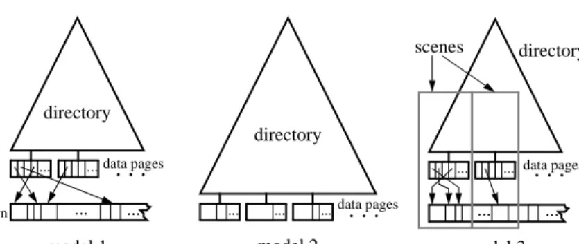
Basically, there are three different models for storing spatial objects:
1.) Storing the exact object representations outside of the data pages (model 1) In the data pages of the index structure, we store the approximations and the pointers to the exact representations of the objects. The exact representation is stored outside the index structure, e.g. in a sequential file. This approach is used in quadtrees for instance [HS 92]. In other words, the spatial index structure is a primary index for the approximations and a secondary index for the spatial ob-jects. This model is shown schematically in figure 10. The main advantage of this scheme is the large number of approximations stored together in one data page, i.e. a maximum degree of local ordering of the approximations is pre-served. Furthermore, there is no limit to the size of the exact object representa-tion. A fundamental drawback is the fact that the order preservation just refers to the object approximations and not to the objects themselves. Consequently, when processing range queries for each access to an exact object representation an additional page access is necessary.
2.) Storing the exact object representation inside the data pages (model 2) The exact representation of the objects is stored, in addition to the approxima-tions, inside the data pages. Therefore, spatial neighborhood is physically pre-served and objects are transferred into main memory just using one disk access [Wid 91]. In contrast to the first model, the index structure is a primary index for the spatial objects and determines their storage location. An essential drawback of this approach is the low number of objects fitting into one page. As a conse-quence, neighboring objects are often stored in different pages. In section 2.2 we have emphasized that objects larger than one data page often occur in geographic databases. Handling these objects with the second model is a difficult task be-cause a special page overflow mechanism has to be implemented.
3.) Storing objects in a scene organization (model 3)
This model has already been presented in section 4.4. Larger parts of the data are physically clustered within so called scenes and organized in an R*-tree. In figure 10 the three models are depicted.
The scene organization has been designed for supporting large region queries. Con-sidering such set-oriented queries, we have to take a closer look to two important prob-lems:
• Which performance is gained by the three models ? Is the performance of the scene organization superior to the other two models ?
• Which size of the scenes leads to the best query performance ? Does this size sig-nificantly depend on the size of the range queries ?
Fig. 10. Models for storing spatial objects Test environment
To find an answer to these questions, we have carried out a detailed empirical perform-ance comparison of the three models. We used real test data from the US Bureau of the Census [Bur 89] containing county borders, highways, railway connections and rivers of four Californian counties. This database consists of 119.151 lines, each consisting of 2 to 349 points. Each co-ordinate is represented by a real number of 8 Bytes. Altogether the database has a size of 15.9 MByte. The lines were approximated by using minimal bounding boxes. For the representation of these boxes 16 Bytes are available. These boxes are depicted in figure 11 (a).
Fig. 11. Data and queries used for the tests
Using this data set we built up three R*-trees referring to the three different models. The page capacity was 4 KByte.
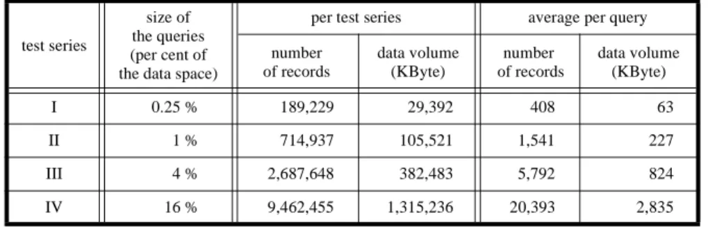
To investigate the performance of the models for large query regions, we carried out four test series with different sizes of the query regions. Each series consists of 464 quadratic window queries uniformly distributed over the data space covered by the ob-jects. The area of the query regions varies between 0.25% and 16% of the data space. In figure 11 (b) the 1% queries are shown. Table 1 presents the query specification of the four test series.
data pages ... ...
. . .
... ... ...
. . .
... ...
. . .
scenes
model 1 model 2 model 3
... ... ... ...
directory
directory
directory
extern data pages
data pages
To evaluate the performance of the three models, we need a measure for the access cost. The time necessary for reading one page into main memory consists of the search time, i.e. the time needed for locating the page on secondary storage, and the transfer time, i.e. the time needed to transfer the data from secondary into main memory. Normalize the cost for a transfer operation to 1. Then in real magnetic disk drives the cost for a search operation is approximately 10 [PH 90]. If NS denotes the number of search op-erations and NT denotes the number of transfer operations then the complete access cost A is given by:
Considering range queries, the access cost within the R*-tree is negligible in compari-son to the access cost of the exact object representation. Thus, in the following, we take into account only the access cost for reading the exact object representation.
Test results:
In table 2, we present the access cost when storing the lines outside the data pages (model 1). The number of search operations (NS), the number of transfers (NT) and the access cost A are presented (in the following table, A is not directly calculated from NS and NT due to rounding).
Storing the exact object representation outside the data page, requires at least one (ex-pensive) search operation for each answer, because of the missing spatial organization of the exact object representations.
Table 3 contains the results for model 2, i.e. for storing the lines inside the data pages.
test series
size of the queries (per cent of the data space)
per test series average per query number of records data volume (KByte) number of records data volume (KByte) I 0.25 % 189,229 29,392 408 63 II 1 % 714,937 105,521 1,541 227 III 4 % 2,687,648 382,483 5,792 824 IV 16 % 9,462,455 1,315,236 20,393 2,835
Tab. 1. Characteristics of the test series
test series I (0,25 %) test series II (1 %) test series III (4 %) test series IV (16 %) NS NT A NS NT A NS NT A NS NT A
189 189 2,082 715 715 7,864 2,688 2,689 29,585 9,462 9,463 104,088
Tab. 2. Access cost for model 1 (in thousand, rounded)
test series I (0,25 %) test series II (1 %) test series III (4 %) test series IV (16 %) NS NT A NS NT A NS NT A NS NT A
16 16 175 52 52 573 180 180 1,985 610 610 6,710
Tab. 3. Access cost for model 2 (in thousand, rounded) A = 10NS+NT
Compared to model 1, model 2 needs considerably less search operations. The reason for this behavior is the fact that many neighboring objects are stored in just one data page and read into main memory by one access. The improvement only marginally de-pends on the size of the query ranges. NT has basically the same size as NS, because in the test data only a few records are larger than one page.
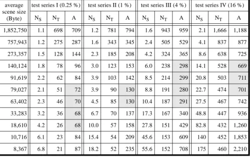
In the scene organization (model 3), the results considerably depend on the average size of the scenes. Using model 1, the exact object representation is only accessed if it is necessary for query processing. Contrarily, in the second model exact object repre-sentations are read into the main memory if they are close to the margin of the query region, but do not intersect the query region (false hits). Large scenes need only a small number of search operations but a high number of transfers from the secondary to the main memory due to the large number of false hits. On the other hand, the smaller the scenes, the higher the effort for searching and the lower the number of transfers. To ex-amine this effect in more detail and to determine the optimal scene size, we varied the scene size in our comparisons. The results are presented in table 4 where the best results are shaded.
As expected, with increasing scene size NS decreases and NT increases. Scene sizes be-tween 25 and 100 KByte lead to minimum access cost, depending on the size of the que-ries. The larger the queries, the larger the optimal scene size. However, this dependency is not as strong as expected. There is a factor of 64 in the size of the queries between test series I and IV, but only a factor of 4 in the resulting optimal scene sizes. Addition-ally, the graphs for the cost functions are very flat close to their minimum. Thus, we chose 77 KByte as a nearly optimal scene size for all test series.
Conclusion
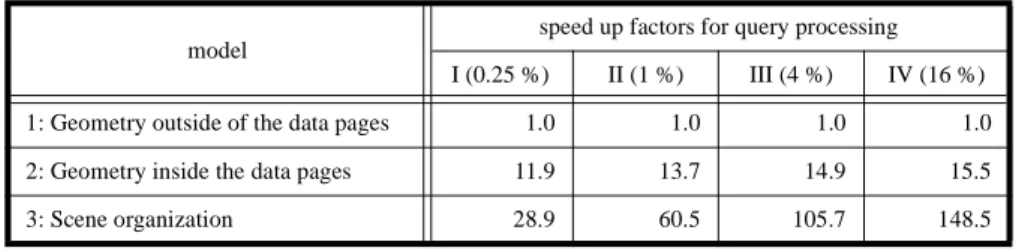
In table 5, the access cost for all three models is presented. The cost for model 1 is stand-ardized to “1”. For the other two models the numbers describe the speed up factor for
average scene size
(Byte)
test series I (0.25 %) test series II (1 %) test series III (4 %) test series IV (16 %) NS NT A NS NT A NS NT A NS NT A 1,852,750 1.1 698 709 1.2 781 794 1.6 943 959 2.1 1,666 1,188 757,943 1.2 275 287 1.6 343 345 2.4 505 529 4.1 837 877 273,357 1.5 128 144 2.3 185 208 4.2 324 365 8.6 638 725 140,124 1.8 78 96 3.0 123 153 6.0 238 298 14.1 528 669 91,619 2.2 62 84 3.9 103 142 8.5 214 299 20.8 503 711 79,027 2.1 51 72 3.9 90 130 8.8 191 280 22.7 474 701 63,402 2.3 46 70 4.5 85 130 10.4 187 291 27.5 467 742 33,283 3.2 36 68 6.7 70 137 17.3 167 340 48.8 447 936 18,610 4.2 26 68 10.0 57 158 27.8 151 429 82.8 432 1,260 10,716 6.1 23 84 15.4 54 209 45.6 153 609 140 452 1,853 8,367 6.8 21 87 18.2 52 235 55.6 152 708 175 460 2,210
query processing using these models. The average scene size for model 3 is 79,027 Bytes.
In conclusion, we would like to point out the following statements:
• Storing the exact object representation inside the data pages (model 2) speeds up query processing by a factor of 12 to 15 in comparison to model 1 (using separate pages). The size of the query regions has only a small influence on this factor. For the interpretation of the results one remark is important: The objects used for the tests are relatively small in comparison to the size of the data pages. Using larger objects, i.e. objects larger than one data page, requires storing the exact representa-tion outside of the data pages. As a consequence, query performance of model 2 comes closer to the performance of model 1.
• The new scene organization is the clear winner of the performance comparison. Even the processing of small queries is performed considerably faster by this stor-age model. For small queries, we have a speed up factor of about 30 (in comparison to model 1) which is increasing to the impressive value of 148 for large queries. Another important result is the fact that the optimal scene size is almost independent of the query sizes. Therefore, using the scene architecture with a fixed scene size is beneficial to queries of very different size.
Furthermore, the flat form of the cost function guarantees a considerable speed up of the query processing, even if the average size of the scene is varying caused by insertions and deletions of objects.
6 Conclusion
We proposed a storage and access architecture for geographic database systems. This architecture integrates a number of various concepts and techniques for efficient query processing.
The R*-tree is the basic component of our geo architecture. It organizes the data on secondary storage with respect to their spatial location and shape. In this way, the search region of spatial queries can be quickly narrowed down. The next ingredient of our ar-chitecture are object approximations. They support an efficient preselection to decide whether an object fulfills the query or not. In comparison to the usually used minimum bounding box, the minimum 5-corner is a good compromise between the quality of the approximation and the amount of required storage. The exact geometric representation of an object is managed by a TR*-tree. The polygonal objects are decomposed into sim-pler components and organized with respect to their spatial location and shape. This al-lows a selective access to the components needed to process a spatial query. Due to the simplicity of the components, the application of time consuming computational geometry algorithms to complex objects is avoided. Thematic queries are supported by
model
speed up factors for query processing I (0.25 %) II (1 %) III (4 %) IV (16 %) 1: Geometry outside of the data pages 1.0 1.0 1.0 1.0 2: Geometry inside the data pages 11.9 13.7 14.9 15.5 3: Scene organization 28.9 60.5 105.7 148.5
secondary indices for thematic attributes. These secondary indices are connected to the primary index, i.e. the R*-tree, using a link table.
The parts of our architecture mentioned above support efficient processing of que-ries with high spatial selectivity, i.e. point queque-ries and small window queque-ries. To speed up the set-oriented object access of large range queries, we added a new ingredient to our architecture: the scene organization. Using this new approach, large parts of the data are combined in scenes and spatially clustered on secondary storage. These scenes are organized within the primary R*-tree. We investigated the performance of this ap-proach in a detailed performance comparison. For large range queries, the scene organ-ization is superior in performance to ordinary storage models with a speed up factor up to two orders of magnitude.
The use of our architecture is not restricted to geographic information systems. With only slight modifications it can also be used in systems for computer aided design (CAD) or computer integrated manufacturing (CIM).
In our future work, we plan to incorporate our geo architecture into an existing ex-tensible database system for spatial applications. Promising candidates for this idea are DASDBS, GRAL and POSTGRES. Performance evaluations of our geo architecture af-ter incorporating it into such a system will be very inaf-teresting.
Furthermore the design of a parallel geo architecture is an interesting challenge for future research activities. Parallelism should be exploited in two ways. First, we want to use a multi processor system to process queries in main memory in a massively par-allel way. Using object decomposition techniques in a parpar-allel environment promises a considerable performance improvement. Second, we want to use multi disk systems to organize the large data volume of geographic applications more efficiently. The main problem to solve is, to determine an appropriate distribution of the data over the differ-ent disk drives.
The application of the presented techniques to 3D-objects is another interesting field of research activities for the future. For example, bio-computing is an important field of application for 3D-spatial objects. The first step in this direction is the development and implementation of 3D-approximation and decomposition techniques.
References
[Aro 91] Aronoff S.: ‘Geographic Information Systems’, WDL Publications, 1991.
[Bar 88] Bartelme N.: ‘GIS Technology: Geographic information systems, land information
systems and their fundamentals’ (in German), Springer, 1988.
[BKS 93a] Brinkhoff T., Kriegel H.-P., Schneider R.: ‘Comparison of Approximations of
Com-plex Objects used for Approximation-based Query Processing in Spatial Database Systems’, Proc. 9th Int. Conf. on Data Engineering, Vienna, Austria, 1993.
[BKS 93b] Brinkhoff T., Kriegel H.-P., Schneider R.: ‘Scene Organization: A Technique for
Global Clustering in Spatial Database Systems’, 1993, submitted for publication.
[BKSS 90] Beckmann N., Kriegel H.-P., Schneider R., Seeger B.: ‘The R*-tree: An Efficient and
Robust Access Method for Points and Rectangles’, Proc. ACM SIGMOD Int. Conf.
on Management of Data, Atlantic City, NJ., 1990, pp. 322-331.
[Bur 86] Burrough P.A.: ‘Principles of Geographical Information Systems for Land
Re-sources Assessment’, Oxford University Press, 1986.
[Bur 89] Bureau of the Census: ‘TIGER/Line Percensus Files, 1990 Technical
[CDRS 86] Carey M. J., DeWitt D. J., Richardson J. E., Shekita E. J.: ‘Object and File
Manage-ment in the EXODUS Extensible Database System’, Proc. 12th Int. Conf. on Very
Large Data Bases, Kyoto, Japan, 1986, pp. 91-100.
[Cra 90] Crain I.K.: ‘Extremely Large Spatial Information Systems - A Quantitative
Perspec-tive’, Proc. 4th Int. Symp. on Spatial Data Handling, Zürich, Switzerland, 1990,
pp. 632-641.
[Fra 91] Frank, A.U.: ‘Properties of Geographic Data’, Proc. 2nd Symp. on Large Spatial Databases, Zürich, Switzerland, 1991, in: Lecture Notes in Computer Science, Vol. 525, Springer, 1991, pp. 225-234.
[GC 87] Gorny A.J., Carter R.: ‘World Data Bank II: General users guide’, Technical report, U.S. Central Intelligence Agency, Washington, 1987.
[Gut 84] Guttman A.: ‘R-trees: A Dynamic Index Structure for Spatial Searching’, Proc. ACM SIGMOD Int. Conf. on Management of Data, Boston, MA., 1984, pp. 47-57. [Güt 89] Güting R. H.: ‘Gral: an extensible relational database system for geografic
applica-tions’, Proc. 15th Int. Conf. on Very Large Data Bases, Amsterdam, Netherland,
1989, pp. 33-44.
[HS 92] Hoel E.G., Samet H.: ‘A Qualitative Comparison Study of Data Structures for Large
Line Segment Databases’, Proc. SIGMOD Conf., San Diego, CA., 1992,
pp 205-214.
[HSW 88] Hutflesz A., Six H.-W., Widmayer P.: ‘Globally Order Preserving Multidimensional
Linear Hashing’, Proc. 4th Int. Conf. on Data Engineering, Los Angeles, CA., 1988,
pp. 572-579.
[HWZ 91] Hutflesz A., Widmayer P., Zimmermann C.: ‘Global Order Makes Spatial Access
Faster’, Int. Workshop on Database Management Systems for Geographical
Appli-cations, Capri, Italy, 1991, in: Geographic Database Management Systems, Springer, 1992, pp. 161-176.
[KBS 91] Kriegel H.-P., Brinkhoff T., Schneider R.: ‘An Efficient Map Overlay Algorithm
based on Spatial Access Methods and Computational Geometry’, Int. Workshop on
Database Management Systems for Geographical Applications, Capri, Italy, 1991, in: Geographic Database Management Systems, Springer, 1992, pp. 194-211. [KHS 91] Kriegel H.-P., Horn H., Schiwietz M.: ‘The Performance of Object Decomposition
Techniques for Spatial Query Processing’, Proc. 2nd Symp. on Large Spatial
Data-bases, Zürich, Switzerland, 1991, in: Lecture Notes in Computer Science, Vol. 525, Springer, 1991, pp. 257-276.
[Kri 91a] Kriegel H.-P., Heep P., Heep S., Schiwietz M., Schneider R.: ‘An Access Method
Based Query Processor for Spatial Database Systems’, Int. Workshop on Database
Management Systems for Geographical Applications, Capri, Italy, 1991, in: Geo-graphic Database Management Systems, Springer, 1992, pp. 273-292.
[Kri 91b] Kriegel H.-P., Heep P., Heep S., Schiwietz M., Schneider R.: ‘A Flexible and
Exten-sible Index Manager for Spatial Database Systems’, Proc. 2nd Int. Conf. on
Data-base and Expert Systems Applications, Berlin, Germany, 1991, pp. 179-184. [Ore 89] Orenstein J. A.: ‘Redundancy in Spatial Databases’, Proc. ACM SIGMOD Int.
Conf. on Management of Data, Portland, USA, 1989, pp. 294-305.
[PH 90] Paterson D., Hennessy J.: ‘Computer Architecture: A Quantitative Approach’, Mor-gan Kaufman, 1990.
[PS 88] Preparata F.P., Shamos M.I.: ‘Computational Geometry’, Springer, 1988.
[Sam 90] Samet H.: ‘The Design and Analysis of Spatial Data Structures’, Addison Wesley, 1990.
[Sch 92] Schneider R.: ‘A Storage and Access Structure for Spatial Database Systems’, Ph.D.-thesis (in German), Institute for Computer Science, University of Munich, 1992.
[SK 91] Schneider R., Kriegel H.-P.: ‘The TR*-tree: A New Representation of Polygonal
Ob-jects Supporting Spatial Queries and Operations’, Proc. 7th Workshop on
Compu-tational Geometry, Bern, Switzerland, 1991, in: Lecture Notes in Computer Science, Vol. 553, Springer, 1991, pp. 249-264.
[SR 86] Stonebraker M., Rowe L.: ‘The Design of POSTGRES’, Proc. ACM SIGMOD Conf. on Management of Data, Washinton D.C., 1986.
[SV 89] Scholl M., Voisard A.: ‘Thematic Map Modelling’, Proc. 1st Symp. on the Design and Implementation of Large Spatial Databases, Santa Barbara, CA., 1989, in: Lec-ture Notes in Computer Science, Vol. 409, Springer, 1990, pp. 167-190.
[SW 86] Schek H.-J., Waterfeld W.: ‘A Database Kernel System for Geoscientific
Applica-tions’, Proc. 2nd Int. Symp. on Spatial Data Handling, Seattle, Washington, 1986,
pp. 273-288.
[Wei 89] Weikum G.: ‘Set-Oriented Disk Access to Large Complex Objects’, Proc. 5th Int. Conf. on Data Engineering, Los Angeles, CA., 1989, pp. 426-433.
[Wid 91] Widmayer P.: ‘Data Structures for Spatial Databases’ (in German) in: Vossen G., Witt K.-U. (eds.): ‘Entwicklungstendenzen bei Datenbank-Systemen’ (Future Trends in Database Systems), Oldenbourg, 1991, pp. 317-361.