Transportation cost estimation in freight distribution services with time windows: application to an Italian urban area

(1)

Transportation cost estimation in freight distribution

services with time windows: application to an Italian

urban area

Francesco P. Deflorio, Jesus Gonzalez-Feliu, Guido Perboli, Roberto Tadei

To cite this version:

Francesco P. Deflorio, Jesus Gonzalez-Feliu, Guido Perboli, Roberto Tadei. Transportation cost estimation in freight distribution services with time windows: application to an Italian urban area. The Sixth International Conference on City Logistics, Jun 2009, Puerto Vallarta, Mexico. pp.555-568, 2009. <halshs-00758245>

HAL Id: halshs-00758245

https://halshs.archives-ouvertes.fr/halshs-00758245

Submitted on 3 Feb 2013

HAL is a multi-disciplinary open access archive for the deposit and dissemination of sci-entific research documents, whether they are pub-lished or not. The documents may come from teaching and research institutions in France or abroad, or from public or private research centers.

L’archive ouverte pluridisciplinaire HAL, est destinée au dépôt et à la diffusion de documents scientifiques de niveau recherche, publiés ou non, émanant des établissements d’enseignement et de recherche fran¸cais ou étrangers, des laboratoires publics ou privés.

(2)

Transportation cost estimation in freight distribution services with time windows 555

38

T

RANSPORTATION

C

OST

E

STIMATION IN

F

REIGHT

D

ISTRIBUTION

S

ERVICES WITH

T

IME

W

INDOWS:

A

PPLICATION TO AN

I

TALIAN

U

RBAN

A

REA

Francesco P. Deflorio, DITIC,Politecnico di Torino, Turin, Italy

Jesus Gonzalez-Feliu, Laboratoire d’Economie des Transports, Lyon, France Guido Perboli, DAUIN, Politecnico di Torino, Turin, Italy

Roberto Tadei, DAUIN, Politecnico di Torino, Turin, Italy

ABSTRACT

This paper studies a set of indicators for evaluating how the quality of a freight distribution service with time windows, which operates on a given road network to satisfy a number of requests, affects the service cost. The result of a service quality setting, expressed as the width of the time windows, has been assessed using five indicators, which are a measure of the service operating costs and based on the request compatibility time interval. Each indicator’s performance has been evaluated in an experimental context to produce realistic test cases, using a trip planning tool and a demand generator. The results confirm the ability of the selected indicators to predict with a good approximation the transportation costs and therefore to support the service quality planning decisions.

INTRODUCTION

The freight transportation sector is continuously changing as a consequence of the growth and transformation of the economic activity. In recent years companies have reduced their storage areas to reduce costs, and customers have increased their needs of service quality in terms of freight availability and prediction of the delivery times. Moreover, the new advances in technology have been a positive factor for the development of new markets and new consumer needs, one of the most relevant is the “just in time” policy in freight distribution, and in urban context in particular.

In Italy, several small and middle-sized cities have developed city logistics applications with success (Spinedi et al., 2008). Padova (about 200.000 inhabitants) is one of the most know

(3)

556 City Logistics VI

examples. Their system, CityPorto, based on an Urban Distribution Centre (UDC), from where small low-pollution vehicles enter the city central area for picking up or delivering goods at the different retailers. The system has been adapted to other six Italian cities that cover small-sized cities like Aosta (approximately 35000 inhabitants) to middle-sized urban areas, like Modena or Venice (near 400000 inhabitants). Similar systems have been adopted in middle-sized urban areas (from 100000 to 500000 inhabitants). Vicenza and Ferrara are some examples of successful city logistics systems in Italy which follow a similar UDC strategy.

One of the most challenging questions in freight transportation is to ensure the efficiency while maintaining a service quality defined by the time windows or other quality indices. In freight transportation, service quality is often related to travel time, and can vary according to both socio-economic and trip characteristics. Time constraints, which are important in applications such as express courier carriers, postal services, newspaper distribution, and e-commerce, have been considered in vehicle routing problems with time windows (VRP-TW). This problem has been largely studied (Laporte, 1992; Toth and Vigo, 2002b; Cordeau et al., 2007) and several algorithms and variants have been formulated to represent and optimise different real world distribution cases (Cordeau et al., 2001; Toth and Vigo, 2003; Prins, 2004; Ando and Taniguchi, 2006; Pissinger and Ropke, 2007; Perboli et al., 2008; Qureshi et al., 2008). One of the most well studied is the VRP with Time Windows (VRPTW).

In time constrained freight distribution, the high number of carriers and the strong competition between different companies make quality and price important aspects. These two factors are usually related: the higher the quality, the higher the cost incurred. For a transportation carrier, variable costs depend on transportation times, also affected by the total distance travelled by the vehicles. Usually, the dispatching of the requests is managed by specialized software able to optimize the single VRP problems. If this kind of software can deal with the needs of each single freight distribution company, methods for supporting the global service planning and cost forecasting are needed when different actors are involved. The tools available in the literature are usually highly customized to each single application and need highly trained staff. In the past decade, the City Logistics approach started to think the distribution of the freight in urban areas as a whole system. Unfortunately, the complexity of the relationships between the actors, the size (thousands of requests) and the diversification of the freight requests, as well as the different freight typology do not let to directly apply existing methods. Moreover, the tactical decisions are usually taken by stakeholders requiring simple and reliable tools for supporting their decisions.

In this paper we study the set of indicators presented in Deflorio et al. (2008) on a realistic urban freight distribution system, in order to evaluate how a given transport service configuration operating on a given network, is related to its transportation cost. This framework, based on predictive indicators, is simple to understand and to apply even by non-OR experts, can be computed with a limited computational effort, even on large systems, and as we will show on a large set of test instances, gives a good estimation of the total transportation costs trends. The framework is based on the definition of indicators, measuring the level of compatibility between the different requests on the network.

The paper is organized as follows. The basic definitions and the indicators are defined in the next two sections. Then, we describe the simulation settings and testing procedure, based on realistic scenarios considering the network configuration characteristics, as well as service time

(4)

Transportation cost estimation in freight distribution services with time windows 557

and respect of delivery constraints as quality aspects. Finally, the computation results and the evaluation of the performance of the indicators are given.

DEFINITIONS AND NOTATION

In time constrained transport problems, a number of freight requests within a given geographical area have to be satisfied, using a fleet of vehicles to visit them by travelling on a road network in which travel times are assumed to be constant. Each request r is characterized by its corresponding node of the network, the freight amount to be delivered and a time window defined by an Early Arrival Time (EATR), and a Late Arrival Time (LATR). The

vehicle fleet is homogeneous and consists in NVTOT vehicles with the same loading capacity K.

To satisfy a request, the service must deliver the freight by respecting the time constraints. The result of this planning activity or, in other words, how the requests are combined, depends on the level of compatibility of the requests.

Fischetti et al. (2001) define the request compatibility of a pair of requests i and j as a binary attribute whose value is equal to 1 if a feasible circuit visiting the destination point of request i before request j exits; 0 otherwise. Using this attribute we can determine whether request i can be served before request j with the same vehicle, consecutively or not. However, we cannot use it to compare the compatible cases, in order to establish priorities, or determine how flexible is this compatibility or incompatibility.

In a previous work (Deflorio et al., 2008), this concept has been extended by defining the concept of Compatibility Time Interval (CTI) between two requests, defined as follows. Consider two requests rA and rB. The distance in time between A and B is known as tAB and the

time used for loading and unloading operations at the request location, respectively tA and tB.

Let us suppose that we want to serve A and B, according to their time windows, consecutively and we want to calculate the earliest arrival time from A to satisfy this condition. The vehicle will arrive at A at least at EATA and will not leave A beforeEATA+ tA. To ensure request B is

satisfied,, the vehicle must not arrive at B before EATB. The time between arrival at A the

arrival at B is therefore tA+tAB. The early arrival time at A of a vehicle serving A and B

consecutively can be written in the following way :

EATA/B = max {EATA , EATB – (tA + tAB)}

In a similar way, the vehicle cannot arrive at A after LATA and must arrive at B before LATB,

considering the travel time tAB and the time for loading and unloading operations at A, tA. The

latest arrival time at A which will consent a vehicle to serve consecutively A and B is: LATA/B = min {LATA, LATB – (tA + tAB)}

The CTI of the pair of requests A-B is therefore defined as the interval between the earliest arrival time and the latest arrival time at A with a vehicle that needs to deliver to A and B consecutively. We can write a CTI according to the following expression :

CTI A/B = LATA/B - EATA/B

The term CTIA/B can be positive or negative. If CTIA/B is positive, then request rA can precede

request rB directly. The higher the numeric value, the higher the overlapping time interval of

the requests and the easier it will be to serve them with the same vehicle. If CTIA/B is negative,

(5)

• Early arrival at B: A precedes B with a time interval which is bigger than tAB, i.e.

LATA < EATB – (tA+tAB). It is however possible to satisfy rB after rA in the same vehicle

trip, for example delivering to other customers between A and B or making a vehicle stop (slack pause) in order to arrive at B within its TW interval. This possibility is quantified by the value of CTIA/B: if this value is high, it will be more difficult to serve

A and B using the same vehicle.

• Late arrival at B: B precedes A, so it is impossible to carry out the sequence AB in the indicated sequence, i.e. EATB– (tA+tAB)< EATA. In this case it is not possible to visit A

before B in the same vehicle trip, so rA cannot be satisfied before rB if not they are not

visited using different vehicles.

The compatibility time interval for each pair of requests can be collected into a square matrix of dimension nR (the total number of requests to be satisfied). This matrix is called Request

Compatibility Matrix (RCM). To define this matrix, it has been decided to sort the requests in increasing Earliest Arrival Time, to separate the negative compatibilities with the two different meanings. In this way, the negative compatibilities in the upper diagonal indicates the early arrival incompatibilities. The negative elements under the main diagonal identify the late arrival incompatibilities.

PROPOSED INDICATORS

From the RCM, several indicators can be defined (Deflorio et al., 2008). We group these indicators into two sets, one containing statistical indicators, which are obtained by statistical calculations applying average operations, and route-based indicators, which are obtained after route construction heuristics. We present below the three chosen statistical indicators, then we describe briefly the procedure which is used to calculate the two route-based indicators.

The overall Average Compatibility Time Interval (ACTI) represents the average value of all the positive CTIs, including those related to the depot. If we define the number of positive CTIA/B n+S, the ACTI indicator can be formulated as follows:

The percentage of positive CTIs in the RCM is an easily interpretable indicator. Noted as PPC, it is defined using the following expression:

(%) / RCM in elements of number CTI positive of number PPC = A B

Finally, we can calculate for each request rA, the minimum travel time tAB, considering each

request rB compatible with rA. This value is defined as the Minimum Travel Time between rA

and any compatible request rB. Then, the average for the overall set of requests, is called

Average of the Minimum Time Between each request A and any Compatible Request B, and noted AMTBCR. + >

∑

= S CTI B A n CTI ACTI AB 0 / /

(6)

Transportation cost estimation in freight distribution services with time windows 559

( )

R A AB CTI n t AMTBCR AB

∑

> = min_/ 0

The first indicator, ACTI, quantifies the average compatibility time intervals between the requests, the second one, PPC, shows the proportion between positive and negative CTI’s and the third indicator, AMTBCR, gives an estimation of the time required to connect two requests in a plan. Note that these indicators based on the compatibility are calculated for pairs of requests, so they give an initial idea of how the request configuration fits on the network features. The indicators do not however represent well the entire system complexity and the influence of vehicle capacity. For this reason, to extract from the RCM information which was more suitable for our problem, we defined two further indicators: NVI and TI. Using the RCM

it is possible to apply a partitioning to the set of requests and create a number of subsets which can be served in a feasible sequence. We should recall that here the aim is not to find an optimal solution for the distribution service, but to define a measure for the assessment of the compatibility of different requests, which depends on the demand characteristics also in relation to the road network. We built a greedy algorithm in order to produce such feasible sequences of requests grouped in different subsets. If each subset in our problem is viewed as a vehicle with a fixed capacity, then each sequence of requests represents a route for the vehicle. For a detailed description of the algorithm see Deflorio et al. (2008).

From the RCM to each couple A-B we use the values of CTIA/B and assume that request rB can

be satisfied consecutively after rA if:

• the compatibility time interval CTIA/B is positive;

• there is not a slack pause between the requests;

• the vehicle capacity constraints are respected.

To generate a realistic configuration for the sub-set of requests, from each request, among all the possible options, we select the next request of the subset according to the best partial solution (minimum route travel time criterion). Finally, the result obtained in this way have been assumed to estimate the further two indicators, namely the number of vehicles (NVI ) and

the total transportation time (TI).

The described indicators have been tested on the reference instances proposed in literature for large problems (Homberger and Gehring, 2005) and their performance were promising to describe the difficulty degree of a freight distribution scenario with time windows. Therefore in the following we extend the experimental analysis to confirm their ability in assessing the cost level of a scenario also for realistic networks.

The proposed indicators can be used for tactical planning process, before the optimization phase, for example, when a simulation of the service setting variations is required, also for a large number of operating alternatives. Indeed, when the number of scenarios to be analysed increases, the use of a reliable route planning tool is not always practical, because of its high computation time. Moreover, in the planning process, not all the analysts are used to adequately apply these optimization tools, since these are generally used in the operational phase. Therefore, the proposed indicators, which are quite able to correctly estimate the trend of total travel time of a freight distribution service with time windows, can be profitably used to predict this crucial transportation cost factor (Deflorio et al., 2008). This can be done after a

(7)

simple calibration of a linear regression model that requires to know only a few points, possibly derived from the available previous experiences in the same network, or from an adequate route optimization tool.

SIMULATION

OF REALISTIC CASES

To evaluate the presented indicators and their ability to describe the level of difficulty of planning the requests for realistic situations, we need to define the application context, the tools adopted and the settings we have used in order to produce a suitable set of instances. The performance of a distribution service with time constraints is related to the structure of the demand and its variability in time and space. The sporadic nature of the requests increases the difficulty of tackling the problem with an analytical approach. For this reason, we have used a simulation procedure to generate the demand. In cases where several sets of requests are known from real data, the use of the demand simulation can be avoided.

Analysis Tools and their role in the experimental setting

In this section a brief description of the tools used is given, specifying their role in the comparative analysis of the indicators.

Demand generator

A simulation approach was used to build the demand for the scenarios (Deflorio, 2005). Individual delivery or pickup requests have been generated at nodes of the road network at specific times. Each node can be considered as a possible point where a vehicle can stop and deliver or pickup the freight. Homogeneous nodes can be grouped in zones, so information available on different parts of a geographical area, e.g. macro-descriptive variables, can be used to estimate the ability to generate or attract freight shipments, expressed via generation or attraction indexes.

Trip planning

In order to compare the results of our indicators and study their validity, a trip planning tool is required to solve routing problems with time windows. In this case, we use ILOG Dispatcher, a commercial tool for solving the VRP-TW, able to solve instances of 200 customers or more with a limited computational effort. More in detail, we implemented a Tabu Search procedure with a composite neighbourhood including 2-OPT, request swap between routes and request movement to different vehicles. The Tabu Search stops after 5 non-improving iterations (for further details, see ILOG, 2005).

Scenario characteristics

Road network

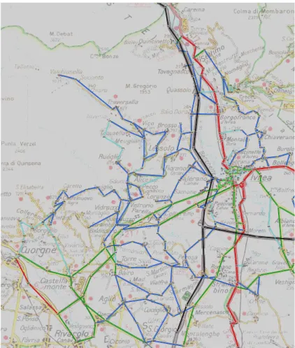
Since the aim is to investigate real-life problems, a real road network is used for the experiments. The road network chosen is located within the Canavese district, in the north of Italy, close to Turin (see Figure 1). This area, which includes the urban area of Ivrea (about 25.000 inhabitants) and its surroundings, which can be considered a urban community with 50000 inhabitants. Although the mostly part of the considered area presents a urban context. A

(8)

Transportation cost estimation in freight distribution services with time windows 561 rural area nearby the main town (Ivrea) is also taken into account, because of the peculiar socio-economic context of the Canavese district.

1 2 3 4 5 6 7 8 9 10111213 14 15 1617 18 19 20 21 22 23 24 25 26 2728 29 3031 32 33 34 35 36 37 38 39 40 41 42 43 44 45 46 47 48 49 50 51 52 53 54 55 56 57 58 72 77 78 79 80 85 86 87 88 89 90 92 93 94 95 96 97 98 99 100 101 102 103 104 105 106 107 108 109 110 111 112 113 114 115 116 117 118119 120 121 122 123 124 125 126 127 128 129 130 131 132 133 134 135 136 137 138 139 140 141 142 143 144 145 146 147 148 149 150 151 152 153 154 155 156 157 158 159 160 161 162 163 164 165 166167 168 169 170 171 172 173 174 175 176 177 178 179 180 181 182 183 184 185 186 187 188 189 190 191 192 193 194 195 196 197 198 199 200 201 202 203 204 205 208 209 210 211 212 213 214 215 216 217 220 222 223 225 226 227 228 233 234 235 236 237 238 240 241 242 243 244 245 246 247 253 254 255 256 257 258 259 260 261 262 263 264 265 266 267 268 269 272 273 274 275 276 277 278 279 280 281 282 283 284 285 286 287 288 289 290 291 292 293 294 295 296 297 302 303 304 305 306 307 308 309 310 311 312 313 316 317 318 319 320 321 322 323 324 325 326 327 328

Figure 1: Road network used in experimental analysis

The graph consists of 330 nodes and 836 oriented links. For each link, distances and travel times are provided. Travel time for each arc are assumed to be constant (since congestion phenomena are not relevant here) considering the distance between two nodes and the type of road, which characterises its average speed. The travel times are expressed in hours. Each node represents the location of a potential customer who can make a freight distribution request.

Demand features

In order to simulate realistic requests we used the demand generator described before. The whole area was divided into 9 zones and attraction and generation indexes used to define the total demand for each zone for the pickup and delivery problem respectively. Given a demand distribution per zone, it is possible to build up different test cases, where each request is located in a specific node belonging to one of the zones. Each node has the same probability as other nodes in the same zone to generate a request, although any zone can have a different probability according to the attraction and generation indexes.

Service features

In the organisation of freight distribution services, we observe two conflictual factors. In order to increase profits, the transportation carriers wish to reduce costs, which means increasing

(9)

service efficiency. However, this can have a negative effect on quality standards and may make it difficult to achieve the level of service expected by the user, who could change provider if the requested quality is not respected. The level of service in our study is defined as respect for the Time Window and measured by its width (the shorter waiting period, the higher the quality of the service). Moreover, the number of vehicles is related to the level of service. In general, carriers have a minimum number of vehicles which suppose a fix cost (even if they are not used) and only the usage of further vehicles will lead to a cost increase. The more complex and restrictive the time windows, the more difficult it becomes to maintain a good level of efficiency.

In our experiments we suppose a transportation carrier using one depot, situated at a node in the road network, and a number of available vehicles for the service equal to 30, in order to allow the complete satisfaction of the request for any scenario. In this phase, we assume that all vehicles have the same capacity, expressed in terms of volume (4.5 m3). Note that for capacity limitations, constraints due to the disposition of the freight inside the vehicles is not taken into account. The time for loading operations at the request location, in the scenarios analysed, has also been taken into account by assuming it equal to 4’ for any request.

Methodology for the experimental analysis

To evaluate the different indicators, we apply them to several sets of simulations. The area of study (Ivrea and surroundings in the Piedmont region) has the particularity to present an urban area build by a small city and a surrounding rural area with even smaller satellite towns (which is the case of many urban areas in Europe). Different scenarios are created by considering one or more of the following elements:

• Network and demand characteristics: geographical position, road characteristics, urban area characteristics, density of potential requests, request distribution within the period length.

• Service organization and quality characteristics represented by the time windows width. For each experiment of any scenario, 100 tests have been made using the travel demand generator, in order to produce a statistical population which can represent several similar but not identical situations (Figure 2). For these replications, we consider a total fixed demand of 200 requests for each experiment. The average demand attraction for each zone is also known. From these parameters, and using the travel demand generator, we obtain 100 random demand extractions. For each extraction, we build a test replication, identifying the corresponding RCM and deriving all the presented indicators. For the same random extraction of requests, using the trip planning tool we obtain the total travel time Tand the number of used vehicles N.

(10)

Figure 2: Chart of the experimental procedure

For each experiment, we can estimate average values and the statistical dispersions for the proposed indicators and the trip planning results, for a high number of cases, since the objective is to explore the validity of the indicators in realistic scenarios.

Test instance definition

To evaluate the indicators presented, we created a number of test instances, which have been used to test the indicators’ behaviour in different realistic situations. Two sets of experiment were set up, each using a different scenario:

• Set 1 - Time Window Width (TWW) based instances. The time interval which defines each request (TWW) has a uniform request distribution profile over time. For each value of TWW between 1 and 4 hours a set of 100 instances have been created.

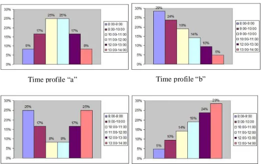
• Set 2 - Time Period Profile (TPP) based instances. The second type of experiment (TPP) focuses on the time distribution of the requests in a given time period. All the time windows have the same width equal to 1h. We use four realistic time profile distributions of the requests (see Figure 3). The time profile “a” simulates the case where a high concentration of requests occurs in the middle of the time period. Time profile “b” represents a demand distribution where a high concentration of requests take place at the beginning of the period, then this concentration gradually decreases. Time profiles “c” and “d” are complementary profiles to “a” and “b”, respectively. For each TPP 100 instances with the requests randomly generated are built.

(11)

Time profile “a”

Time profile “c” Time profile “d”

Time profile “b”

Figure 3: Four realistic cases of time profile

After testing the given indicators on the proposed scenarios, using the VRPTW heuristic as a tool to study their precision and accuracy, we have selected the most relevant indicators to describe the interaction between the proposed service quality and the related transportation costs for the considered distribution strategy. The transportation cost have been estimated by means of the number of vehicles required to satisfy all the requests and their total travel time along the routes.

COMPUTATIONAL RESULTS

In this section we present the main computational results of the two sets of experiments in order to test the chosen indicators in realistic scenarios based on data taken from the area of Ivrea (Italy). The analysis considers two axes. First, we analyse the behaviour of the indicators on the Time Windows Width experiments. Then, we show how they behave in forecasting the total cost of the requests under different Time Period Profiles.

Time Windows Width experiments

We solved each of the four sets of 100 replications of the TWW experiment type, using the ILOG Dispatcher planning tool (ILOG, 2005). The average values for all the 5 indicators described and the trip planning tool results (in number of vehicles and total travel time, respectively N and T) are reported in the columns of the Table 1 for the 4 experiments. The variation of the all average values of indicators is evident over the TWW variation and confirms the trends expected.

(12)

Table 1: Average values of the indicators for Set 1.

Indicators Planning Tool Results

TWW ACTI PPC AMTBCR NV_I T_I N T 1h 1888,33 30,94 154,96 40,15 198412 6,22 66554 2h 3871,85 56,07 114,70 18,00 109515 5,70 55822 3h 6038,77 75,47 99,95 8,91 70360 5,32 49381 4h 8446,97 89,27 91,98 6,25 55438 5,25 46248

Moreover, a detailed data analysis of the dispersion of results allow us to distinguish a different behaviour for the 5 indicators represented on to 5 graphs, one for each of the selected indicators. Each graph has the total travel cost on Y axis, while the indicator value is reported on X. For each size of TWW, the values of the corresponding instances are reported with a different mark. ACTI and PPC (Figure 4) have a similar statistical dispersion, quite low with respect to that one of T. Indeed, if a separation of the 4 data sets is possible, by using the X axe, the same is not possible on the Y axe (total travel time).

40000 45000 50000 55000 60000 65000 70000 75000 80000 0 20 40 60 80 100 T PPC 1h 2h 3h 4h 40000 45000 50000 55000 60000 65000 70000 75000 80000 0 2000 4000 6000 8000 10000 T ACTI 1h 2h 3h 4h

Figure 4: Travel cost (in seconds) related to ACTI and PPC.

On the other hand, AMTBCR, NVI and TI (Figure 5) have a greater statistical dispersion and

describe the same overlapping phenomena observed for T (between the cases 3h and 4h) and a separation of sets for these indicators, as is for T, between the cases 2h and 1h. We can therefore notice how the dispersion of the cost values related to the indicators becomes more and more evident while TWW changes from 1h to 2h. The results also show that AMTBCR, NVI, and TI indicators have a linear-wise increasing trend while the TWW decreases; ACTI

and PPC have an opposite trend. Thus, the results confirm the expected behaviour.

40000 45000 50000 55000 60000 65000 70000 75000 80000 0 50000 100000 150000 200000 250000 300000 T Ti 1h 2h 3h 4h 40000 45000 50000 55000 60000 65000 70000 75000 80000 0 50 100 150 200 T AMTBCR 1h 2h 3h 4h 40000 45000 50000 55000 60000 65000 70000 75000 80000 0 10 20 30 40 50 60 T NVi 1h 2h 3h 4h

(13)

Time Period Profile experiments

We repeated the same simulation method to the four presented time period profiles. In Table 2, we report the average values of the indicators and the planning tool solutions (N, T). The meaning of the columns is the same as in Table 1.

Table 2: Average values of the indicators for Set 2.

Indicators Planning Tool Results

ACTI PPC AMTBCR NVI TI N T a 1858,41 37,19 149,91 38,21 190768 6,18 65433 b 1904,10 36,57 155,37 38,68 193914 6,28 64955 c 1983,06 31,60 154,65 39,73 195546 6,41 65327 d 1908,69 37,07 144,14 38,31 188625 6,33 64901 u 1888,33 30,94 154,96 40,15 198412 6,22 66554

Each row represents the results obtained with the 4 TPP distributions a, b, c, and d. Row u shows the values computed in Set 1, i.e. uniform distribution of TPP and TWW equal to 1h. The profiles a, b, c and d present an average total travel time (T) higher than the uniform one. Thus, the transportation cost of the non-uniform profile cases are in average smaller than the uniform profile case. This behaviour is confirmed, in the experiments performed, also observing the values of ACTI and PPC which have, as desired, their minimum value for the case of uniform TPP (u) and similar higher values for the other 4 profiles. As required, an opposite trend can be observed for NVI and TI, where for the “u” profile the maximum value

has been estimated. For the Set 2 the behaviour of the indicator AMTBCR is not useful, since its trend is not clear. However, the average values of the indicators are quite similar , as well as the trip planning results, for the non-uniform TPP experiments and not all of the indicators are able to describe this particular feature of the instance.

CONCLUSIONS

In this paper we presented a new methodology to evaluate how the quality of the freight distribution service with time windows is related to the characteristics of the road network and the demand. The evaluation methodology defines several indicators, which are based on the definition of Compatibility Time Interval (CTI). These indicators are grouped into two sets: the indicators of the first set are obtained using simple statistical operators, and those of the second group need a route-construction procedure, based on a Nearest Neighbor approach which chooses the best partial solution (following the criterion of minimum route travel time) among all the candidates that assure a feasible solution.

This framework, based on predictive indicators, is simple to understand and to apply even by non-OR experts. It can be computed with a limited computational effort, even on large systems, and as we have shown on a large set of test instances, it gives a good estimation of the total transportation costs trends. We would also like to remark that indicators can be computed very quickly and they are defined without the need of any parameters to be set or calibrated, since they should be “impartial” measurements and standard references to classify scenarios to

(14)

Transportation cost estimation in freight distribution services with time windows 567 improve the simple information contained in time windows width. On the contrary, any trip planning solution derives from the choice of parameters in the objective function.

In the experimental procedure presented, the indicators have been statistically studied in a number of scenarios with time windows width and time period profile variations. Extensive computational results, based on 800 VRPTW instances, show the effectiveness of the indicators in order to predict the expected total transportation cost.

Further experimental analysis could be carried out in order to explore the indicator behaviour in predicting cost variations of freight distribution services operating on instances deriving from the fusion of different data sets of requests. This could represent an approximation in a simulated environment of the case where different operators in the same geographical area would share their freight requests in a city logistics context.

ACKNOWLEDGMENTS

We would like to thank anonymous referees for helpful comments on the paper.

REFERENCES

Ando, N., and Taniguchi, E. (2006). Travel Time Reliability in Vehicle Routing and Scheduling with Time Windows, Networks and Spatial Economics 6, pp. 293-311. Braysy, O. and Gendreau, M. (2005). Vehicle Routing Problem with Time Windows, Part I:

Construction and Local Search Algorithms. Transportation Science 39-1, 104-118. Braysy, O. and Gendreau M (2005). Vehicle Routing Problem with Time Windows, Part II:

Metaheuristics. Transportation Science 39-1, 119-139.

Cordeau, J. F., Laporte, G. and Mercier, A. (2001). A unified tabu search heuristic for vehicle routing problems with time windows, Journal of the Operational Research Society 52, pp. 928-936.

Cordeau, J. F., Laporte, G., Savelsberg, M. and Vigo D. (2007). Vehicle Routing. In: C. Barnhart, G. Laporte (Eds.), Transportation, North Holland Elsevier, pp. 367–428. Deflorio, F. P. (2005). La simulazione delle richieste di viaggio nei sistemi di trasporto a

chiamata. In G. E. Cantarella; F. Russo, Metodi e tecnologie dell'ingegneria dei trasporti,

Seminario 2002, Franco Angeli (ITA), pp. 186-199.

Deflorio, F. P., Gonzalez-Feliu, J., Tadei, R. and Amico, S. (2008). Service quality planning for freight distribution with time windows in large networks. Technical Report Politecnico di Torino.

Fischetti, M., Lodi, A., Martello, S. and Toth, P. (2001). A Polyhedral Approach to Simplified Crew Scheduling and Vehicle Scheduling Problems. Management Science 47 (6), 833-839.

Homberger, J. and Gehring, H. (2005). A two-phase hybrid metaheuristic for the vehicle routing problem with time windows, European Journal of Operational Research 162, pp. 220-238.

ILOG (2005), ILOG Dispatcher 4.0 Manual, ILOG, France.

Perboli, G., Pezzella, F. and Tadei, R. (2008) EVE-OPT: an Hybrid Algorithm for the Capability Vehicle Routing Problem, Mathematical Methods of Operations Research vol. 68, pp. 361-382.

Pissinger, D. and Ropke S. (2007). A general heuristic for vehicle routing problems, Computers & Operations Research 34, pp. 2403-2435.

(15)

Prins, C. (2004) A simple and effective evolutionary algorithm for the vehicle routing problem, Computers & Operations Research 31, pp. 1985–2002.

Qureshi, A. G., Taniguchi, E. and Yamada, T. (2008). A hybrid genetic algorithm for VRPSTW using column generation. In Taniguchi, E. and Thomson, R. G., Innovations

in City Logistics, Nova Science Publishers, pp. 151-166.

Spinedi, M., Ambrosino, G., Pandolfo, P and Vaghi, C. (2008) Logistica urbana: dagli aspetti

teorici alle applicazioni, RER-City Logistics Expo, Bologna, Italy.

Toth, P. and Vigo, D. (2002). The vehicle routing problem, SIAM Monographs on Discrete Mathematics and Applications, vol. 9, Philadelphia, USA.

Toth, P. and Vigo, D. (2003). The granular tabu search and its application to the vehicle routing problem, Journal on Computing 15, pp. 333-346.