UNIVERSITY OF OKLAHOMA GRADUATE COLLEGE
DISTRIBUTED COMPUTATION OF GRAPH SPECTRUM, EIGENVECTOR CENTRALITY,
AND SOLUTION TO LINEAR EQUATIONS
A DISSERTATION
SUBMITTED TO THE GRADUATE FACULTY in partial fulfillment of the requirements for the
Degree of DOCTOR OF PHILOSOPHY By MU YANG Norman, Oklahoma 2017
DISTRIBUTED COMPUTATION OF GRAPH SPECTRUM, EIGENVECTOR CENTRALITY,
AND SOLUTION TO LINEAR EQUATIONS A DISSERTATION APPROVED FOR THE
SCHOOL OF ELECTRICAL AND COMPUTER ENGINEERING
BY
Dr. Choon Yik Tang, Chair
Dr. J. R. Cruz
Dr. S. Lakshmivarahan
Dr. Thordur Runolfsson
c
⃝Copyright by MU YANG 2017 All Rights Reserved.
Acknowledgements
Firstly, I would like to express my sincere gratitude to my advisor, Dr. Choon Yik Tang, for providing tremendous mentoring and support throughout my Ph.D. studies. He gave me freedom to pursue my own research interests and at the same time provided me with valuable feedback and advice. Besides research, he also gave me insightful suggestions on my career and life.
I am grateful to Dr. J. R. Cruz, Dr. S. Lakshmivarahan, Dr. Thordur Runolfsson, and Dr. Krishnaiyan Thulasiraman for their interest in my research and for serving on my dissertation committee. I have greatly benefited from their involvement and recommendations.
I would like to thank my family. My wife, Jingjue Yi, has been extremely supportive of me throughout this entire process and has made countless sacri-fices to help me get to this point. My daughter, Harper, has continually brought me happiness. My parents, Chengfeng Yang and Yafei Lin, always have faith in me and give me liberty to choose what I desired. Special thanks to my father-and mother-in-law, Yong Yi father-and Huiping Liu, who came to Norman twice father-and helped us take care of Harper.
Finally, financial support from the National Science Foundation is grate-fully acknowledged.
Table of Contents
Acknowledgements iv
List of Figures vii
Abstract viii
Chapter 1. Introduction 1
1.1 Background and Motivation . . . 1
1.2 Literature Review . . . 2
1.3 Original Contributions . . . 4
1.4 Dissertation Outline . . . 6
Chapter 2. Distributed Estimation of Graph Spectrum 7 2.1 Introduction . . . 7
2.2 Problem Formulation . . . 9
2.3 Forming a Set of Linear Equations . . . 11
2.4 Solving the Linear Equations . . . 16
2.4.1 Scenario 1: Cyclic Case . . . 16
2.4.2 Scenario 2: Acyclic Case . . . 21
2.5 Simulation Results . . . 24
2.5.1 Simulation of Algorithm 2.1 for Scenario 1 . . . 24
2.5.2 Simulation of Algorithm 2.2 for Scenario 2 . . . 26
2.6 Conclusion . . . 28
Chapter 3. A Distributed Algorithm for Solving General Linear Equations 29 3.1 Introduction . . . 29
3.2 Problem Formulation . . . 31
3.4 Algorithm Analysis . . . 34
3.5 Convergence Rate Analysis . . . 42
3.5.1 Proof of Theorem 3.4 . . . 45
3.5.2 Why Convergence may be Slow . . . 52
3.6 Simulation Results . . . 53
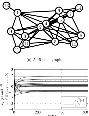
3.6.1 Two 15-Node Graphs . . . 54
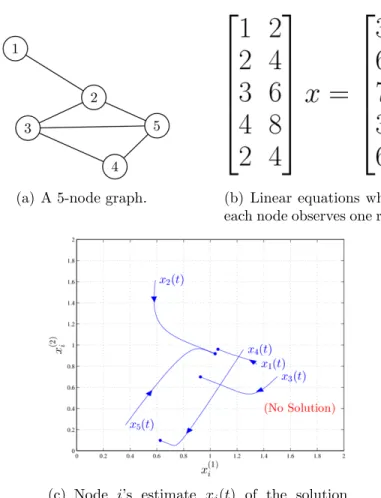
3.6.2 A 5-Node Graph . . . 55
3.7 Conclusion . . . 55
Chapter 4. Continuous-Time Distributed Computation of the Perron-Frobenius Eigenvector 62 4.1 Introduction . . . 62
4.2 Problem Formulation . . . 64
4.3 Design of Continuous-Time Algorithms . . . 67
4.4 Analysis of Continuous-Time Algorithms . . . 71
4.4.1 Convergence Analysis . . . 71
4.4.2 Convergence Rate . . . 77
4.4.3 Special Cases . . . 88
4.5 Simulation Results . . . 90
4.6 Conclusion . . . 90
Chapter 5. Asynchronous Gossip Computation of the Perron-Frobenius Eigenvector 92 5.1 Introduction . . . 92
5.2 Problem Formulation . . . 93
5.3 Design of Gossip Algorithm . . . 94
5.4 Analysis of Gossip Algorithm . . . 99
5.5 Simulation Results . . . 110 5.6 Conclusion . . . 110 Chapter 6. Conclusions 113 6.1 Overall Summary . . . 113 6.2 Future Work . . . 115 Bibliography 118
List of Figures
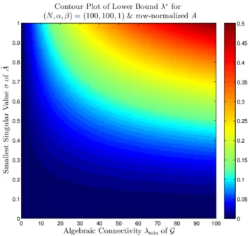
2.1 Distribution of the eigenvalues of a graph’s adjacency matrix, represented by red crosses, offers insights into the shapes and sizes of communities in the graph. . . 8 2.2 Flowchart illustrating our approach to estimating graph spectrum. 10 2.3 Performance of Algorithm 2.1 for Scenario 1. . . 25 2.4 Performance of Algorithm 2.2 for Scenario 2. . . 27 3.1 Illustration of the idea behind algorithm (3.5). . . 33 3.2 Contour plot showing how the lower bound λ∗ on the
conver-gence rateλ1of algorithm (3.7) depends on the smallest singular
valueσ of ˆA and the algebraic connectivity λmin(L) of G, when
(N, α, β) = (100,100,1). . . 45 3.3 A simple example explaining why algorithm (3.7) may converge
slowly whenA is nearly singular. . . 53 3.4 Performance of algorithm (3.6) when there is a unique solution. 57 3.5 Performance of algorithm (3.6) when there is no solution. . . 58 3.6 Performance of algorithm (3.6) when there is no solution. . . 59 3.7 Performance of algorithm (3.6) when there is a unique solution. 60 3.8 Performance of algorithm (3.6) when there are infinitely many
solutions. . . 61 4.1 Examples illustrating the concept of eigenvector centrality. . . . 63 4.2 Vector field for a 3-node path graph. . . 73 4.3 Performance of continuous-time algorithm (4.12). . . 91 5.1 Performance of gossip algorithm. . . 112
Abstract
DISTRIBUTED COMPUTATION OF GRAPH SPECTRUM, EIGENVECTOR CENTRALITY,
AND SOLUTION TO LINEAR EQUATIONS
Mu Yang, Ph.D.
The University of Oklahoma, 2017
Supervisor: Choon Yik Tang
This dissertation is devoted to the development of distributed algorithms, with which nodes in a large decentralized network can accomplish tasks that are seemingly difficult without an omniscient central node. The tasks include esti-mating the graph spectrum, from which each node can draw its own conclusion about the network structure, computing the eigenvector centrality, from which every node can judge its own importance in the network, and solving a system of linear equations whose data are scattered across the network or discovering that no solution exists. The ability to perform these tasks enhances the ca-pability of existing and emerging networks such as smart power grids, social networks, and ad hoc sensor networks, potentially allowing them to function in ways that are not previously thought to be possible.
We begin with the design of a novel, two-stage distributed algorithm that enables nodes in an undirected and connected graph to jointly estimate the spectrum of a matrix associated with the graph, which includes the adjacency and Laplacian matrices as special cases. In the first stage, the algorithm uses a discrete-time linear iteration and the Cayley-Hamilton theorem to convert
the problem into one of solving linear equations, where each equation is known to a node. In the second stage, if the nodes happen to know that said matrix is cyclic, the algorithm uses a Lyapunov approach to asymptotically solve the equations with an exponential rate of convergence. Otherwise, it uses a random perturbation approach and a structural controllability result to approximately solve the equations with an error that can be made small.
We then consider the fundamental problem of cooperatively solving a general system of linear equations over a network, for which a continuous-time distributed algorithm is devised. We show that the algorithm enables the nodes to asymptotically agree on a solution when there are infinitely many solutions, determine the solution when there is exactly one, and detect that no solution exists when there are none. We also establish that the algorithm is globally exponentially convergent, derive an explicit lower bound on its convergence rate that it can do no worse than, and prove that the larger the network’s algebraic connectivity, or the further away from being singular the system of equations, the larger this lower bound.
Finally, we address the open question of whether it is possible to calcu-late eigenvector centrality over a network. We provide an affirmative answer by presenting a class of continuous-time distributed algorithms and an asyn-chronous gossip algorithm, which allow every nodeiin a graph to compute the ith entry of the Perron-Frobenius eigenvector of a symmetric, Metzler, and ir-reducible matrix induced by the graph, as well as the corresponding eigenvalue, when node i knows only row i of the matrix. We show that each continuous-time distributed algorithm is a nonlinear networked dynamical system with a skew-symmetric structure, whose state is guaranteed to stay on a sphere, re-main nonnegative, and converge asymptotically to said eigenvector at an O(1t)
rate. We also show that under a mild assumption on the gossiping pattern, the gossip algorithm is able to do the same.
Chapter 1
Introduction
1.1 Background and Motivation
Recent years have witnessed a tremendous growth in the types and ap-plications of networked systems. From a network of computers and cell phones that form the Internet and cellular networks in the last couple of decades, to a network of tiny wireless sensors and huge wind turbines that monitor activ-ities and generate renewable energy in the past few years, networked systems continue to change the way we live. Indeed, new types and applications of such systems (e.g., social networks) continue to emerge, offering potential that captures the fascination of scientists and engineers.
In many emerging and future applications of networked systems, systems in the network—commonly referred to interchangeably as nodes or agents— often have to cooperatively accomplish sophisticated tasks that require exten-sive sharing and rapid processing of information, as well as optimal formulation and precise coordination of actions, under a variety of constraints and uncer-tainties. For instance, sensors in a wireless network typically have to com-municate in multi-hop fashion over unreliable physical channels for as long as possible, despite facing severe bandwidth and battery constraints. Therefore, although such networked systems offer promising potential, their design and operation are very challenging, to say the least.
A key factor that adds significantly to the challenge is the fact that in many of these networked systems, for various practical reasons it is often not feasible, or not advisable, to have a powerful centralized node, who knows all about the network topology and makes all the necessary decisions. For example, with the aforementioned wireless sensor network, transmitting information from every node and relaying it back to the centralized node may be too costly from a bandwidth and battery standpoint. Such transmission and relay is also vulnerable to node mobility and single-point failures, making it necessary to frequently maintain an overlay tree rooted at the centralized node, which maybe costly. Likewise, for networks deployed in battlefields and for social networks, doing so may simply be impermissible for vulnerability, security, and privacy reasons. As a result, the nodes must interact locally—perhaps only with immediately neighboring nodes—autonomously and collaboratively performing the tasks as if a centralized node is present. It follows that distributed (or decentralized) algorithms, which define how the nodes should locally interact, are critical to effectively realizing a variety of networked systems.
1.2 Literature Review
Recognizing the pressing need for distributed algorithms, researchers from a number of scientific and engineering disciplines (e.g., systems and con-trol, computer science, operation research) have invested a great deal of re-search efforts in designing and analyzing such algorithms. In the field of sys-tems and control, the efforts may be roughly grouped into three overlapping areas, namely, distributed consensus, distributed computation, and distributed optimization.
In distributed consensus, nodes or agents in a network seek to achieve an agreement on what they individually observe or experience. The agreement may be completely arbitrary (e.g., a platoon of vehicles may want to agree on a direction along which they all move), or it may be constrained to be some form of weighted average (e.g., a set of temperature sensors may want to determine the average of their individual temperature measurements). Be-ing able to achieve such an agreement is often the basis of cooperation in a distributed system. Due to its significance, the distributed consensus problem has been widely studied in the literature, resulting in a rich collection of dis-tributed algorithms in continuous-time (e.g., [1–13]) and in discrete-time with synchronous (e.g., [1,3,6–9,11,14–31]) and asynchronous (e.g., [20,32–50]) time models. In addition, such algorithms have been tailored to a variety of engi-neering applications, including but not limited to motion coordination [51], vehicle formation [52, 53], and flocking [43, 54, 55].
In distributed computation, nodes in a network seek to compute a global, non-trivial quantity of common interest, whose value depends on either the graph topology or the scattered node observations. In this area, a growing number of problems have been addressed to date. Over the past decade, for example, notable research efforts have been devoted to the distributed com-putation of maximum [34, 37, 56–58], sum/count [14, 33, 34, 57], power mean [34, 56, 59], resource redistribution [15], Kalman filters gains [12, 60–63], lin-ear functions [28, 64–66], average-max-min [2], log-sum-exp [58], and a class of general functions [56, 59, 67]. More recently, some attention has been given to distributed computation of betweenness and closeness centrality [68–72], the spectrum of a graph and its corresponding eigenvectors [73–79], and the solu-tion to linear equasolu-tions [31, 62, 80–87].
Finally, in distributed optimization, each node typically observes a local, often convex, objective function and some local constraints, and all of the nodes wish to find an optimizer that minimizes the sum of their local objective functions subject to satisfying all their local constraints. This problem has an emerging number of applications, including to power grids [88–90], smart buildings [91, 92], and sensor networks [93, 94]. Motivated by its potential, the problem has been gaining much attention, leading to a large collection of distributed algorithms such as the incremental subgradient algorithms [93, 95–102], non-incremental ones [31, 103–110], zero-gradient-sum algorithms [50, 111–116], and various other algorithms [117–120].
1.3 Original Contributions
In this dissertation, we add to the growing literature on distributed com-putation by focusing on three specific problems of considerable significance: distributed computation of the spectrum of a graph, the solution to general linear equations, and the Perron-Frobenius eigenvector. Our original contribu-tions can be summarized as follows.
First, we construct a novel, two-stage distributed algorithm that enables nodes in an undirected and connected graph to jointly estimate the spectrum of a matrix associated with the graph, which includes its adjacency and Laplacian matrices as special cases. Knowledge of the spectrum allows the nodes to infer about the graph structure. In the first stage, the algorithm uses a discrete-time linear iteration and the Cayley-Hamilton theorem to convert the problem into one of solving a set of linear equations, where each equation is known to a node. In the second stage, if the nodes happen to know that said matrix is cyclic, the
algorithm uses a Lyapunov approach to asymptotically solve the equations with an exponential rate of convergence. If they do not know whether said matrix is cyclic, the algorithm uses a random perturbation approach and a structural controllability result to approximately solve the equations with an error that can be made small.
Second, we design a continuous-time distributed algorithm that allows nodes in an undirected and connected graph to collaboratively solve a general system of linear equations, where the only assumption is that each equation is known to at least one node. We show that the algorithm enables the nodes to asymptotically agree on a solution when there are infinitely many solutions, determine the solution when there is exactly one, and discover that no solution exists when there are none. In addition, we prove that the algorithm is globally exponentially convergent, derive an explicit lower bound on its convergence rate, and show that under certain conditions, the larger the graph’s algebraic connectivity, or the further away from being singular the system of equations, the larger this lower bound.
Third, we devise a class of continuous-time distributed algorithms, which enable each node i in an undirected and connected graph to compute the ith entry of the Perron-Frobenius eigenvector of a symmetric, Metzler, and irre-ducible matrix associated with the graph, as well as the corresponding eigen-value, when nodei knows only row i of the matrix. Knowledge of such entries allows the nodes to determine their eigenvector centrality representing their rel-ative importance in the graph. We show that each continuous-time distributed algorithm in the class is a nonlinear networked dynamical system with a skew-symmetric structure, whose state is guaranteed to stay on a sphere, remain nonnegative, and converge asymptotically to said eigenvector at an O(1t) rate.
We also show that the same idea that yields the continuous-time algorithms can be extended to a discrete-time setting, leading to an asynchronous gossip algorithm for computing the Perron-Frobenius eigenvector, which is provably asymptotically convergent at an O(1k) rate under a mild assumption on the gossiping pattern.
1.4 Dissertation Outline
The outline of this dissertation is as follows: Chapter 2 studies dis-tributed estimation of graph spectrum, in which a two-stage algorithm is devel-oped. Chapter 3 constructs a continuous-time distributed algorithm for solving general linear equations over networks. Chapters 4 and 5 address the problem of distributed computation of the Perron-Frobenius eigenvector. In particu-lar, Chapter 4 presents a class of continuous-time solutions, while Chapter 5 presents an asynchronous gossip counterpart. Finally, Chapter 6 concludes the dissertation and suggests a number of possible extensions as future work.
Chapter 2
Distributed Estimation of Graph Spectrum
2.1 Introduction
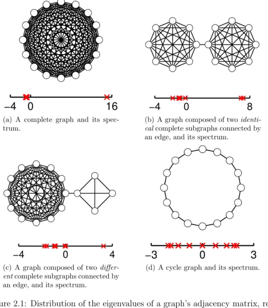
The spectrum of a graph, defined as the set of eigenvalues of either its adjacency or Laplacian matrix, provide a useful characterization of the prop-erties of the graph. For instance, as illustrated in Figure 2.1, the distribution of such eigenvalues offers insights into the shapes and sizes of communities in a network [121]. Indeed, for the complete graph depicted in Figure 2.1(a), its eigenvalues form two distinct clusters, with the first cluster having one dominant, positive eigenvalue and the second cluster having the rest of the eigenvalues concentrated around −1. For the barely connected graphs with two communities in Figures 2.1(b) and 2.1(c), their eigenvalues also form two clusters, but the clusters are much closer to each other, and there may be ei-ther one or two dominant, positive eigenvalues in the first cluster. For the cycle graph in Figure 2.1(d), its eigenvalues are more or less uniformly distributed over an interval centered at zero. As another example, the largest and smallest of such eigenvalues provides bounds on the maximum, minimum, and average node degrees [122]. The spectrum of a graph has also been used, for exam-ple, in chemistry, where it is associated with the stability of molecules [122], and in quantum mechanics, where it is related to the energy of Hamiltonian systems [122].
(a) A complete graph and its spec-trum.
(b) A graph composed of two identi-calcomplete subgraphs connected by an edge, and its spectrum.
(c) A graph composed of two differ-entcomplete subgraphs connected by an edge, and its spectrum.
(d) A cycle graph and its spectrum.
Figure 2.1: Distribution of the eigenvalues of a graph’s adjacency matrix, rep-resented by red crosses, offers insights into the shapes and sizes of communities in the graph.
increasingly complex networks, it is becoming desirable that nodes in a network have the ability to analyze the network themselves, such as decentralizedly computing the spectrum of the network, so that valuable understanding about, say, the network structure may be gained. Motivated by this, a number of distributed algorithms have been proposed in the literature, including [123–125] that consider estimation of the entire spectrum of the Laplacian matrix, and
[77–79] that focus on estimation of its second smallest eigenvalue (i.e., the algebraic connectivity).
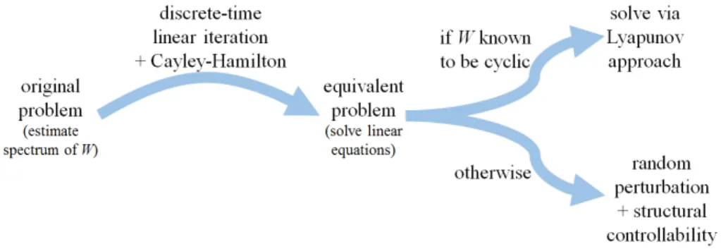
In this chapter, we add to the literature by developing a two-stage distributed algorithm, which enables nodes in a graph to cooperatively es-timate the spectrum of a matrix W associated with the graph. Unlike in [77–79, 123–125], the matrix W can be the adjacency or Laplacian matrix of the graph, a weighted version of these matrices, or any other matrix induced by the graph (see Chapter 2.2). To construct the algorithm, we first use a discrete-time linear iteration and the Cayley-Hamilton theorem to convert the original problem into an equivalent problem of solving a set of linear equations of the form Ax = b, where every row of A and b is known to a particular node (Chapter 2.3). We then show that the matrix A can be made almost surely nonsingular if the nodes happen to know that W is cyclic, but not nec-essarily so if they do not (Chapter 2.3). In the case of the former, we use a Lyapunov approach to asymptotically solve the equations with an exponential rate of convergence (Chapter 2.4.1). In the case of the latter, we use a random perturbation approach and a structural controllability result to approximately solve the equations with an error that can be made small (Chapter 2.4.2). A flowchart illustrating the aforementioned approach is depicted in Figure 2.2. Finally, we provide simulation results that demonstrate the effectiveness of our distributed algorithm (Chapter 2.5).
2.2 Problem Formulation
Consider a network modeled as an undirected, connected graph G = (V,E), where V = {1,2, . . . , N} denotes the set of N ≥ 2 nodes and E ⊂
Figure 2.2: Flowchart illustrating our approach to estimating graph spectrum. {{i, j} : i, j ∈ V, i ̸= j} denotes the set of edges. Any two nodes i, j ∈ V are neighbors and can communicate if and only if {i, j} ∈ E. The set of neighbors of each node i∈ V is denoted as Ni ={j ∈ V :{i, j} ∈ E}, and the
communications are assumed to be delay- and error-free, with no quantization. Suppose associated with the graph G is a square matrix W = [wij] ∈ RN×N satisfying the following assumption:
Assumption 2.1. The matrix W is such that for each i, j ∈ V with i̸= j, if {i, j}∈ E/ , then wij =wji = 0.
Note that Assumption 2.1 allows wii ∀i ∈ V to be arbitrary. It also
allows wij and wji ∀{i, j} ∈ E to be arbitrary and different. Thus, W can
be the adjacency or Laplacian matrix of graph G, a weighted version of these matrices, or any other matrix associated with G as long as Assumption 2.1 holds.
Suppose each node i ∈ V knows only Ni, wii, and wij ∀j ∈ Ni, which
it prefers to not share with any of its neighbors due perhaps to security and privacy reasons. Yet, despite having only such local information about the graph G and matrix W, suppose every node i ∈ V wants to determine the
spectrum of W, i.e., all theN eigenvalues of W, denoted as
λ(1), λ(2), . . . , λ(N) ∈C, (2.1) where complex eigenvalues must be in the form of conjugate pairs. Finally, suppose each node i ∈ V knows the value of N, which is not an unreasonable assumption since each of them wants to determine the values of N objects.
Given the above, the goal of this chapter is to devise a distributed algorithm that enables every node i ∈ V to estimate the spectrum (2.1) of W with a guaranteed accuracy.
2.3 Forming a Set of Linear Equations
In this section, we show that by having the nodes execute a discrete-time linear iteration N times, the problem of finding the spectrum (2.1) of W may be converted into one of solving a set of linear equations with appealing properties.
Observe that although none of the nodes has complete information about G and W, each node i ∈ V knows the entire row i of W (since it knows wiiand wij ∀j ∈ Ni, and sincewij = 0 ∀j /∈ {i} ∪ Ni by Assumption 2.1). This
makes the nodes well-suited to carry out the discrete-time linear iteration yi(t+ 1) =wiiyi(t) +
∑
j∈Ni
wijyj(t), ∀i∈ V, ∀t∈Z+, (2.2)
which in matrix form may be written as
y(t+ 1) =W y(t), ∀t ∈Z+, (2.3)
whereZ+ ={0,1,2, . . .},yi(t)∈Ris maintained in nodei’s local memory, and
y(t) = [y1(t) y2(t) · · · yN(t)
]T
Indeed, (2.2) or (2.3) can be implemented by having each nodei∈ Vrepeatedly send its yi(t) to every neighbor j ∈ Ni.
Since (2.3) is a discrete-time linear system, we can write
y(t) = Wty(0), ∀t∈Z+, (2.5)
so that
y(N) =WNy(0). (2.6)
By the Cayley-Hamilton theorem, WN in (2.6) may be expressed as
WN =−x(0)IN −x(1)W − · · · −x(N−1)WN−1, (2.7)
whereIn ∈Rn×n is the identity matrix and the scalarsx(0), x(1), . . . , x(N−1) ∈R
are the N coefficients of the characteristic polynomial of W, i.e., det(λIN −W) = (λ−λ(1))(λ−λ(2))· · ·(λ−λ(N))
=λN +x(N−1)λN−1+· · ·+x(1)λ+x(0). (2.8) Substituting (2.7) into (2.6) and using (2.5), we obtain
y(N) = (−x(0)IN −x(1)W − · · · −x(N−1)WN−1)y(0)
=−x(0)y(0)−x(1)y(1)− · · · −x(N−1)y(N −1). (2.9) By using (2.4), we can rewrite (2.9) as
y1(0) y1(1) · · · y1(N −1) y2(0) y2(1) · · · y2(N −1) .. . ... . .. ... yN(0) yN(1) · · · yN(N −1) | {z } A x(0) x(1) .. . x(N−1) | {z } x∗ = −y1(N) −y2(N) .. . −yN(N) | {z } b , (2.10)
where, for later convenience, we denote the matrix on the left-hand side of (2.10) as A ∈ RN×N, the vector of characteristic polynomial coefficients as x∗ ∈RN, and the vector on the right-hand side of (2.10) as b∈RN.
The matrix equation (2.10) suggests the following approach for finding the spectrum (2.1) of W: suppose each nodei ∈ V selects an initial condition yi(0) ∈R. Upon selecting the yi(0)’s, suppose the nodes execute the
discrete-time linear iteration (2.2) or equivalently (2.3)N times fort ∈ {0,1, . . . , N−1}. During the execution, suppose each node i ∈ V stores the resulting N + 1 numbers yi(0), yi(1), . . . , yi(N − 1), yi(N) in its local memory. Then, (2.10)
is a set of N linear equations in which each node i ∈ V knows the entire row i of A and b, and in which the vector x∗ of N characteristic polynomial coefficients x(0), x(1), . . . , x(N−1) of W are theN unknowns. It follows that ifA is nonsingular, and if the nodes are able to cooperatively solve (2.10) for the unique x∗, then each of them could determine on its own the N eigenvalues λ(1), λ(2), . . . , λ(N) of W using (2.8) and a polynomial root-finding algorithm.
To realize the above approach, it is necessary that A in (2.10) is non-singular. To see whether this can be ensured, observe from (2.4), (2.5), and (2.10) that A may be expressed as
A =[y(0) W y(0) · · · WN−1y(0)]. (2.11) In the form (2.11), A is, interestingly, the controllability matrix of a fictitious discrete-time single-input linear system
z(t+ 1) =W z(t) +y(0)u(t), ∀t∈Z+, (2.12)
where z(t) ∈ RN is its state, u(t)∈ R is its input, W is its state matrix, and y(0) is its input matrix. Hence:
Proposition 2.1. The matrix A in (2.10) or (2.11)is nonsingular if and only if the pair (W, y(0)) of the system (2.12) is controllable.
SinceW is given by the problem buty(0) may be freely selected by the nodes, it may be possible to selecty(0) so that the pair (W, y(0)) is controllable. The following definition and lemmas examine this possibility:
Definition 2.1 ([126]). A square matrix with real entries is said to be cyclic if each of its distinct eigenvalues has a geometric multiplicity of 1.
Lemma 2.1. If W is not cyclic, then for every y(0)∈ RN, the pair (W, y(0))
is not controllable.
Proof. Suppose W is not cyclic and let y(0) ∈ RN be given. Then, by
Defini-tion 2.1,W has an eigenvalueλ∈Cwhose geometric multiplicity exceeds 1, i.e., rank(W−λIN)< N−1. Sincey(0) is a column vector, rank([W−λIN |y(0)])<
N. Therefore, by statements (i) and (iv) of Theorem 3.1 in [126], the pair (W, y(0)) is not controllable.
Lemma 2.2. IfW is cyclic, then for almost everyy(0)∈RN, the pair(W, y(0))
is controllable.
Proof. According to Lemma 3.12 in [126], if A ∈Rn×n is cyclic and B ∈Rn×m
is such that the pair (A,B) is controllable, then for almost every v ∈Rm, the pair (A,Bv) is controllable. Applying this lemma with A =W, B = IN, and
v =y(0), and using the fact that the pair (W, IN) is controllable, we conclude
that so is the pair (W, y(0)).
Proposition 2.1 and Lemma 2.1 imply that W being cyclic is necessary for A in (2.10) or (2.11) to be nonsingular. Lemma 2.2, on the other hand,
implies thatW being cyclic is essentially sufficient because almost everyy(0)∈
RN would work. This latter result is especially useful in a decentralized network
because the result allows each nodei∈ V to select its yi(0)∈R independently
from other nodes and randomly from any continuous probability distribution before executing (2.2) or (2.3), and be almost sure that the resulting A would be nonsingular.
Motivated by the above analysis, in the rest of this chapter we consider separately the following two scenarios:
Scenario 1. The nodes know that W is cyclic.
Scenario 2. The nodes do not know whether W is cyclic, or know that W is not cyclic.
We consider Scenarios 1 and 2 separately because Scenario 1 is easier to deal with (in Chapter 2.4.1) and its treatment helps us deal with Scenario 2 (in Chapter 2.4.2). We note that both of these scenarios arise in applications. For instance, if the graph G represents a sensor network and the entries wii
∀i ∈ V and wij ∀{i, j} ∈ E of W represent random sensor measurements
with continuous probability distributions, then Scenario 1 takes place as the nodes could say with near certainty that W is cyclic because almost every n-by-n matrix has n distinct eigenvalues and, thus, is cyclic. In contrast, if W represents the adjacency or Laplacian matrix of G, then Scenario 2 takes place as W would be cyclic if G is, say, a path graph [122] and would not be cyclic if G is, say, a complete or cycle graph [122], which the nodes could not tell because they only have local information about G.
To summarize, in this section we have transformed the problem of find-ing the spectrum (2.1) ofW into one of solving the set of linear equations (2.10),
in which each node i ∈ V knows the entire row i of A and b, and in which A can be made almost surely nonsingular in Scenario 1, but not necessarily so in Scenario 2.
2.4 Solving the Linear Equations 2.4.1 Scenario 1: Cyclic Case
In this subsection, we focus on Scenario 1 and develop a continuous-time distributed algorithm that enables the nodes to asymptotically solve the set of linear equations (2.10) with an exponential rate of convergence.
To facilitate the development, we assume that the nodes have executed (2.2) or (2.3) to arrive at (2.10). Moreover, since A in (2.10) can be made almost surely nonsingular in this Scenario 1, we assume that it is nonsingular throughout the subsection. With these assumptions, for each i ∈ V let ai =
[ yi(0) yi(1) · · · yi(N −1) ]T ∈RN andb i =−yi(N)∈R, so that (2.10) may be stated as —aT1 — —aT 2 — .. . —aT N — | {z } A x(0) x(1) .. . x(N−1) | {z } x∗ = b1 b2 .. . bN | {z } b , (2.13)
whereai andbiare known to nodeibecause (2.2) or (2.3) has been executed. In
addition to knowing ai and bi, suppose each node i ∈ V maintains in its local
memory an estimate xi(t) =
[
x(0)i (t) x(1)i (t) · · · x(Ni −1)(t)
]T
∈ RN of the
unknown, unique solution x∗ ∈RN, where heret ∈[0,∞) denotes continuous-time (unlike in Chapter 2.3 wheret∈Z+ denotes discrete-time). Furthermore,
let x(t) = (x1(t), x2(t), . . . , xN(t)) ∈ RN
2
be vectors obtained by stacking the N estimates xi(t)’s and N copies of the
solutionx∗.
To come up with a distributed algorithm that gradually drives x(t) to
x∗, consider a quadratic Lyapunov function candidate V : RN2
→ R, defined as V(x) =∑ i∈V αi(aTi xi−bi)2 + ∑ {i,j}∈E β{i,j}(xi−xj)T(xi−xj), (2.14)
where αi > 0 ∀i ∈ V and β{i,j} > 0 ∀{i, j} ∈ E are parameters. Notice that
each term in the first summation in (2.14) is a measure of how far away from the hyperplane{z ∈RN :aTi z =bi}the estimatexi(t) is. Moreover, becauseA
is nonsingular and because of (2.13), the N hyperplanes {z ∈ RN : aTi z = bi}
∀i ∈ V have a unique intersection at x∗. Furthermore, the second summation in (2.14) is a measure of the disagreement among the estimates xi(t)’s. Hence,
both the first and second summations in (2.14) are only positive semidefinite functions of x. However, as the following proposition shows, adding them up makes V a legitimate Lyapunov function candidate:
Proposition 2.2. If A in (2.13) is nonsingular, then the function V in (2.14) is positive definite with respect to x∗.
Proof. Clearly, V is a positive semidefinite function of x. To show that it is positive definite with respect to x∗, we show that V(x) = 0 if and only if
x = x∗. Suppose x = x∗. Then, aTi xi −bi = 0 ∀i ∈ V according to (2.13).
Next, suppose V(x) = 0. Then,
aTi xi =bi, ∀i∈ V, (2.15)
xi =xj, ∀{i, j} ∈ E. (2.16)
Since G is connected, (2.16) implies that there exists ˜x∈RN such that x i = ˜x
∀i∈ V. Substituting this into (2.15), we get aT
i x˜=bi ∀i ∈ V or, equivalently,
A˜x=b. Since A is nonsingular, we have ˜x=x∗, so that x=x∗. Remark 2.1. Notice that V in (2.14) can also be written as
V(x) = (x−x∗)TP(x−x∗), where P =PT ∈RN2×N2
is positive definite and given by
P = α1a1aT1 0 α2a2aT2 . .. 0 αNaNaTN +Lβ⊗IN,
where ⊗ denotes the Kronecker product andLβ = [Lij]∈RN×N is a weighted
Laplacian matrix of G with Lii =
∑
j∈Niβ{i,j}, Lij = −β{i,j} if {i, j} ∈ E, and Lij = 0 ifi̸=j and {i, j}∈ E/ .
With Proposition 2.2 in hand, we next take the time derivative of V along the state trajectory x(t) to obtain
˙ V(x(t)) = 2∑ i∈V [ αi(aTi xi(t)−bi)ai +∑ j∈Ni β{i,j}(xi(t)−xj(t)) ] ˙ xi(t), ∀t∈[0,∞). (2.17)
Examining (2.17), we see that ˙V(x(t)) can be made negative semidefinite—at the very least—by letting each ˙xi(t) be the negative of the expression within
the brackets in (2.17), i.e., ˙ xi(t) = −αi(aTi xi(t)−bi)ai− ∑ j∈Ni β{i,j}(xi(t)−xj(t)), ∀i∈ V, ∀t∈[0,∞). (2.18) The following theorem asserts that the continuous-time system (2.18) possesses an excellent property:
Theorem 2.1. If A in (2.13) is nonsingular, then the system (2.18) has a unique equilibrium point at x∗ that is globally exponentially stable, so that ∀x(0)∈RN2, limt→∞x(t) =x∗, i.e., limt→∞xi(t) =x∗ ∀i∈ V.
Proof. For each i∈ V, setting ˙xi(t) in (2.18) to zero yields
0 = −αi(aTi xi−bi)ai−
∑
j∈Ni
β{i,j}(xi−xj). (2.19)
Summing both sides of (2.19) over i∈ V gives 0 = ∑
i∈V
−αi(aTi xi−bi)ai. (2.20)
Due to (2.13) and to A being nonsingular, the vectors a1, a2, . . . , aN in (2.20)
are linearly independent in RN. Thus,
0 =−αi(aTixi −bi), ∀i∈ V. (2.21)
Substituting (2.21) back into (2.19) results in 0 = ∑
j∈Ni
β{i,j}(xi−xj), ∀i∈ V,
which is equivalent to
where⊗and Lβ have been defined in Remark 2.1. SinceG is connected, (2.22)
implies that xi = ˜x ∀i ∈ V for some ˜x ∈ RN. Substituting this into (2.21)
yields aTi x˜ = bi ∀i ∈ V. Since A is nonsingular, we have ˜x= x∗, i.e., x= x∗.
Hence, the system (2.18) has a unique equilibrium point at x∗. Since for each i∈ V the right-hand side of (2.18) is the negative of the expression within the brackets in (2.17), ˙V(x(t)) is negative definite with respect to x∗. Therefore, the equilibrium point x∗ is globally exponentially stable.
Having established Theorem 2.1, we now relate it back to the original problem of finding the spectrum (2.1) of W. To this end, suppose each node i∈ V maintains in its local memory an estimateλ(ℓ)i (t)∈Cof the unknown,ℓth eigenvalueλ(ℓ)ofW forℓ ∈ {1,2, . . . , N}. Also suppose at each timet∈[0,∞), node i lets its N estimates λ(ℓ)i (t)’s be the roots of an Nth-order polynomial formed by the estimate xi(t) =
[
x(0)i (t) x(1)i (t) · · · x(Ni −1)(t)
]T
that is also stored in its local memory, i.e.,
(λ−λ(1)i (t))(λ−λi(2)(t))· · ·(λ−λ(Ni )(t))
=λN +x(Ni −1)(t)λN−1+· · ·+x(1)i (t)λ+x(0)i (t),
∀i∈ V, ∀t∈[0,∞), (2.23) which can be implemented using a polynomial root-finding algorithm that is embedded in nodei. Then, because (λ(1), λ(2), . . . , λ(N)) in (2.8) is a continuous
function of x∗ and because (λ(1)i (t), λ(2)i (t), . . . , λ(Ni )(t)) in (2.23) is the same continuous function of xi(t), Theorem 2.1 implies that
lim t→∞λ (ℓ) i (t) =λ (ℓ) , ∀i∈ V, ∀ℓ∈ {1,2, . . . , N}. (2.24) Equation (2.24), in turn, implies that the system (2.18) is a continuous-time
distributed algorithm that enables the nodes to asymptotically learn the spec-trum (2.1) of W.
Putting together the development in Sections 2.3 and 2.4.1, we obtain the following two-stage distributed algorithm, which is applicable to this Sce-nario 1:
Algorithm 2.1 (For Scenario 1).
1. Each node i ∈ V selects its yi(0) ∈ R independently from other nodes
and randomly from any continuous probability distribution.
2. Upon completion, the nodes execute (2.2) or (2.3) N times for t ∈ {0,1, . . . , N −1}, so that each node i ∈ V gradually learns the entire row iof A and b in (2.10).
3. Upon completion, the nodes execute (2.18) and (2.23) indefinitely for t ∈ [0,∞), so that each node i ∈ V is able to continuously update its xi(t) and λ
(ℓ)
i (t)’s.
Remark 2.2. The current literature offers a number of distributed algorithms [31, 84–86] that may be used to solve linear equations (2.10). These algorithms are different from (2.18) in that they force the state of each node to stay in an affine set, whereas (2.18) allows the state to freely roam the state space. Additional differences between them are discussed in Chapter 3.1.
2.4.2 Scenario 2: Acyclic Case
In this subsection, we focus on Scenario 2 and provide a slightly different algorithm that enables the nodes to approximately solve (2.10) with an error that can be made small.
do not know whether W is cyclic, or somehow know that W is not cyclic. Consequently, they either do not know whether A in (2.10) is nonsingular, or know that A is singular. Although the nodes could still apply Algorithm 2.1, there is no guarantee that their estimatesxi(t)’s would converge tox∗. One way
to address this issue is to have the nodes randomly perturb the matrixW and vectory(0), so that the resultingAin (2.11) is hopefully nonsingular. Of course, such a random perturbation approach no longer allows them to asymptotically determine the exact spectrum of W. However, getting an estimate of the spectrum of W may be sufficient in some applications. Thus, we will adopt this random perturbation approach in this Scenario 2.
For notational simplicity, let the matrix associated with the graph G be denoted as W = [wij] ∈ RN×N instead of W = [wij], and let W instead
denote a perturbed version of W. In addition, let x(ℓ)’s and λ(ℓ)’s denote,
respectively, the characteristic polynomial coefficients and eigenvalues of W that the nodes wish to determine, and let x(ℓ)’s and λ(ℓ)’s denote those of W as before. Moreover, let the perturbed matrix W be obtained from W in a decentralized manner as follows: prior to executing (2.2) or (2.3), each node i∈ V lets
wii =wii+δii, ∀i∈ V, (2.25)
wij =wij +δij, ∀i∈ V, ∀j ∈ Ni, (2.26)
where the δii’s and δij’s are independent, uniformly distributed random
vari-ables in the interval [−a, a], so that a > 0 represents the perturbation magni-tude. Notice that since wij = 0 ∀i∈ V ∀j /∈ {i} ∪ Ni by Assumption 2.1,
as well. Also note that because the nodes are slated to select their yi(0)’s
independently and randomly from a continuous probability distribution, there is no need to further randomly perturb these yi(0)’s.
The following lemma uses a structural controllability result to show that the aforementioned approach is effective:
Lemma 2.3. If W is as defined in (2.25)–(2.27) and y(0) is as defined in Step 1 of Algorithm 2.1, then A in (2.11) is almost surely nonsingular.
Proof. Reconsider the graph G = (V,E) from Chapter 2.2. Let S ={(A,B)∈
RN×N ×RN : A
ij = 0 if i ̸= j and {i, j} ∈ E}/ and Sc = {(A,B) ∈ S :
(A,B) is controllable} ⊂ S. In addition, let A∗ = diag(1,2, . . . , N) ∈ RN×N
and B∗ ∈ RN be the all-one vector. Then, (A∗,B∗)∈ S according to the
defi-nition of S. Moreover, (A∗,B∗)∈ Sc because the controllability matrix formed
by (A∗,B∗) is a Vandermonde matrix that is nonsingular. These two properties of (A∗,B∗), along with the definition of structural controllability [127], imply that every (A,B) ∈ S is structurally controllable. Next, let (A,B) ∈ S and ϵ >0 be given. Then, by Proposition 1 of [127], there exists (Ac,Bc)∈ Sc such
that ∥A − Ac∥< ϵand ∥B − Bc∥< ϵ. Hence,Sc is a dense subset ofS. Lastly,
note that (W, y(0)) ∈ S due to Assumption 2.1, (2.25)–(2.27), and Step 1 of Algorithm 2.1. SinceScis a dense subset ofS, (W, y(0)) is almost surely inSc.
Therefore, by Proposition 2.1,A in (2.11) is almost surely nonsingular.
As it follows from Lemma 2.3, by having the nodes perform the extra step described in (2.25)–(2.27), the results developed in Sections 2.3 and 2.4.1 become applicable to this Scenario 2. Furthermore, because both the char-acteristic polynomial coefficients and eigenvalues of a matrix are continuous
functions of its entries, by having the nodes decrease the perturbation mag-nitude a toward zero, the differences between the x(ℓ)’s and λ(ℓ)’s of W and the x(ℓ)’s and λ(ℓ)’s of W can be made arbitrarily small, at least in principle. Note, however, that numerical issues may arise when a is too small, or when the resultingA is ill-conditioned. At present, we do not have answers to these numerical issues, and we believe they are important future research directions. Based on the above, we obtain the following two-stage distributed algo-rithm for this Scenario 2:
Algorithm 2.2 (For Scenario 2).
1. Each node i∈ V executes (2.25)–(2.27) to obtain a perturbed matrix W. 2. The remaining steps are identical to those of Algorithm 2.1.
2.5 Simulation Results
In this section, we present two sets of simulation results that demon-strate the effectiveness of Algorithm 2.1 for Scenario 1 and Algorithm 2.2 for Scenario 2.
2.5.1 Simulation of Algorithm 2.1 for Scenario 1
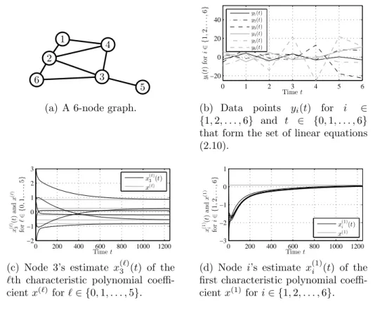
Consider a sensor network with N = 6 nodes, modeled as an undi-rected, connected graphG, whose topology is shown in Figure 2.3(a). Suppose associated with the graph G is a 6-by-6 matrix W, whose entries satisfy
As-1 2 3 4 5 6
(a) A 6-node graph.
0 1 2 3 4 5 6 −20 0 20 40 Timet yi ( t ) fo r i ∈ { 1 , 2 , . . ., 6 } y1(t) y2(t) y3(t) y4(t) y5(t) y6(t)
(b) Data points yi(t) for i ∈
{1,2, . . . ,6} and t ∈ {0,1, . . . ,6}
that form the set of linear equations (2.10). 0 200 400 600 800 1000 1200 −2 −1 0 1 2 3 Timet x ( ℓ ) 3 ( t ) a n d x ( ℓ ) fo r ℓ ∈ { 0 , 1 , . . ., 5 } x(3ℓ)(t) x(ℓ)
(c) Node 3’s estimate x(3ℓ)(t) of the
ℓth characteristic polynomial coeffi-cientx(ℓ)forℓ∈ {0,1, . . . ,5}. 0 200 400 600 800 1000 1200 −3 −2 −1 0 1 Timet x (1 ) i ( t ) a n d x (1 ) fo r i ∈ { 1 , 2 , . . ., 6 } x(1)i (t) x(1)
(d) Node i’s estimate x(1)i (t) of the first characteristic polynomial coeffi-cientx(1) fori∈ {1,2, . . . ,6}. Figure 2.3: Performance of Algorithm 2.1 for Scenario 1. sumption 2.1 and represent random sensor measurements given by
W = −0.10 −0.24 0 0.78 0 0 0.24 0.53 0.39 −0.04 0 −0.19 0 0.34 0.21 1.15 −0.13 0.71 −0.26 −0.21 0.32 −0.54 0 0 0 0 −0.45 0 0.39 0 0 0.47 −0.84 0 0 −1.35 .
Assuming that such measurements are realizations of continuously distributed random variables, the nodes are almost certain that W is cyclic, so that Sce-nario 1 takes place. Thus, to determine all the eigenvalues λ(ℓ)’s of W, which
are given by−1.02±0.55i,−0.004±0.46i, 0.38, and 0.81, the nodes may apply Algorithm 2.1.
Figures 2.3(b)–2.3(d) display the result of simulating Algorithm 2.1 with αi = 10∀i∈ V andβ{i,j} = 10∀{i, j} ∈ E. Specifically, Figure 2.3(b) shows the
data pointsyi(t) fori∈ {1,2, . . . ,6}andt ∈ {0,1, . . . ,6}that are used to form
the set of linear equations (2.10). Figure 2.3(c) shows, as a function of time t, node 3’s estimate x(ℓ)3 (t) of the ℓth characteristic polynomial coefficientx(ℓ) of W forℓ ∈ {0,1, . . . ,5}. Likewise, Figure 2.3(d) shows node i’s estimatex(1)i (t) of the first coefficient x(1) fori ∈ {1,2, . . . ,6}. (Note that instead of including
plots of x(ℓ)i (t) for all i ∈ {1,2, . . . ,6} and ℓ ∈ {0,1, . . . ,5}, we included only two representative ones, in Figures 2.3(c) and 2.3(d).) Observe that despite having only local information about G and W, the nodes are able to utilize Algorithm 2.1 to asymptotically determine all the characteristic polynomial coefficients x(ℓ)’s ofW and, hence, all its eigenvalues λ(ℓ)’s.
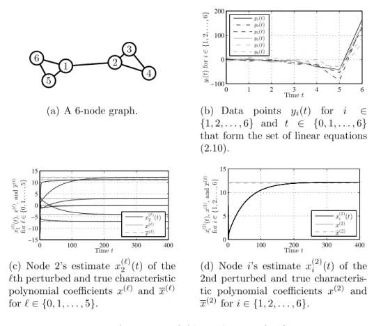
2.5.2 Simulation of Algorithm 2.2 for Scenario 2
Consider next an undirected, connected graph G with N = 6 nodes, whose topology is shown in Figure 2.4(a). Let W represent the adjacency matrix of G and suppose the nodes wish to determine all the eigenvalues λ(ℓ)’s of W, which are given by −1.73, −1,−1, −0.41, 1.73, and 2.41. Because they only have local information about G, the nodes do not know whether W is cyclic, so that Scenario 2 takes place. (In fact, W in this particular example is not cyclic because it is symmetric and has repeated eigenvalues, at −1.) Therefore, the nodes have to apply Algorithm 2.2. In doing so, they let the perturbation magnitude bea = 0.2 and obtain from (2.25)–(2.27) a perturbed matrix W given by W = 0 1.04 0 0 1.01 0.94 0.98 0 1.04 1.12 0 0 0 0.98 0 1.06 0 0 0 0.95 1.01 0 0 0 0.98 0 0 0 0 1.01 0.97 0 0 0 0.92 0 ,
1 2 3
4 5
6
(a) A 6-node graph.
0 1 2 3 4 5 6 −100 0 100 200 Timet yi ( t ) fo r i ∈ { 1 , 2 , . . ., 6 } y1(t) y2(t) y3(t) y4(t) y5(t) y6(t)
(b) Data points yi(t) for i ∈
{1,2, . . . ,6} and t ∈ {0,1, . . . ,6}
that form the set of linear equations (2.10). 0 100 200 300 400 −15 −10 −5 0 5 10 15 Timet x ( ℓ ) 2 ( t ), x ( ℓ ), a n d x ( ℓ ) fo r ℓ ∈ { 0 , 1 , . . ., 5 } x(2ℓ)(t) x(ℓ) x(ℓ)
(c) Node 2’s estimate x(2ℓ)(t) of the
ℓth perturbed and true characteristic polynomial coefficients x(ℓ) and x(ℓ) forℓ∈ {0,1, . . . ,5}. 0 100 200 300 400 0 5 10 15 Timet x (2 ) i ( t ), x (2 ), a n d x (2 ) fo r i ∈ { 1 , 2 , . . ., 6 } x(2)i (t) x(2) x(2)
(d) Node i’s estimate x(2)i (t) of the 2nd perturbed and true characteris-tic polynomial coefficients x(2) and
x(2) fori∈ {1,2, . . . ,6}. Figure 2.4: Performance of Algorithm 2.2 for Scenario 2.
whose eigenvaluesλ(ℓ)’s are −1.74, −0.97, −1.03, −0.40, 1.73, and 2.43, which are all distinct and slightly different from the eigenvalues λ(ℓ)’s ofW.
Figures 2.4(b)–2.4(d) display the result of simulating Algorithm 2.2 with αi = 100 ∀i ∈ V and β{i,j} = 10 ∀{i, j} ∈ E, using a format similar to that
of Figures 2.3(b)–2.3(d). The only difference is that Figures 2.4(c) and 2.4(d) show not only the characteristic polynomial coefficientsx(ℓ)’s of the “perturbed” W, but also the characteristic polynomial coefficients x(ℓ)’s of the “true” W. Observe that with Algorithm 2.2, the nodes are able to asymptotically de-termine the x(ℓ)’s and λ(ℓ)’s. In other words, they are able to approximately
2.6 Conclusion
In this chapter, we have designed and analyzed a two-stage distributed algorithm that enables nodes in a graph to cooperatively estimate the graph spectrum. We have shown that asymptotically accurate estimation can be achieved if the nodes know that the associated matrix is cyclic, and estimation with small errors can be achieved if they do not.
Chapter 3
A Distributed Algorithm for Solving
General Linear Equations
3.1 Introduction
Solving a system of linear equations is a fundamental problem with countless applications. In this chapter, we address the problem of solving such equations over a network, where the equation data are scattered across the network. More specifically, we consider an undirected and connected graph withN nodes, accompanied by a system ofmlinear equations withnunknowns of the form
Ax=b, (3.1)
where each row of A ∈ Rm×n and b ∈ Rm is known to at least one node, and
where every node wishes to find a solution x∈Rn to (3.1), whenever it exists. Since each node knows only part of the equation data, none of them could solve (3.1) on its own. As a result, the nodes must cooperatively do so, preferably in a distributed fashion and preferably without having to share their equation data with others.
This chapter is intended to create an algorithm that equips the nodes with such capabilities. We develop a continuous-time distributed algorithm that allows the nodes to solve a general form of (3.1), where the number of nodesN, number of equationsm, and number of unknownsnmay be arbitrary.
In addition, the existence and uniqueness of a solutionx are not assumed and not known by the nodes in advance, the set Ki of rows of A and b known
to each node i may be arbitrary or even empty, and the only restriction is that every row of A and b is known to one or more nodes. We show that the algorithm enables the nodes to asymptotically agree on a solution when (3.1) has infinitely many solutions, and asymptotically determine the solution when (3.1) has exactly one. We also show that the algorithm enables at least one pair of neighboring nodes to asymptotically discover that no solution exists when (3.1) has none. Moreover, we prove that the algorithm—which is an affine networked dynamical system—is globally exponentially convergent and derive an explicit lower bound on its convergence rate, which it can do no worse than. Furthermore, we show that whenA is square and nonsingular and when each row of A and b is known to exactly one node, the larger the algebraic connectivity of the graph, or the larger the smallest singular value of A(which is its distance to the nearest singular matrix), the larger this lower bound.
We note that the current literature offers a number of distributed al-gorithms for solving (3.1), including those reported in [31, 84–86]. The results in [31, 84–86], however, are different from the ones in this chapter in at least three ways: first, the graphs considered in [31, 84–86] may be directed with time-varying topologies, whereas the one considered here has to be undirected with a fixed topology. Second, the algorithms proposed in [31, 84–86] force the state of each node to stay in an affine set, following the idea ofconstrained con-sensus. In contrast, the algorithm here allows the state to freely roam the state space. Third, the convergence rate result here captures not only the impact of the graph topology, but also that of the problem (e.g., how close to being parallel the rows of A are). The latter is not captured in [31, 84–86]. Lastly,
we note that there is a related line of work [82, 83, 87] on solving (3.1), but the setup is different: in [82, 83, 87], A = ∑Ni=1Ai and b =
∑N
i=1bi, where Ai is a
symmetric positive definite matrix and bi is a vector, both known to and only
to node i.
The outline of this chapter is as follows: Chapter 3.2 formulates the problem. Chapters 3.3 and 3.4 design and analyze the algorithm. Chapter 3.5 analyzes its convergence rate. Finally, Chapter 3.7 concludes the chapter.
3.2 Problem Formulation
Consider a network modeled as an undirected, connected graph G = (V,E), where V = {1,2, . . . , N} denotes the set of N ≥ 2 nodes and E ⊂ {{i, j} : i, j ∈ V, i ̸= j} denotes the set of edges. Any two nodes i, j ∈ V are neighbors and can communicate if and only if {i, j} ∈ E. The set of neighbors of each node i∈ V is denoted as Ni ={j ∈ V :{i, j} ∈ E}, and the
communications are assumed to be delay- and error-free, with no quantization. Suppose associated with the graph G is a system of linear equations Ax =Y, which has m ≥ 1 equations and n ≥ 1 unknowns, and which can be partitioned as —aT 1 — —aT2 — .. . —aTm — | {z } A x= y1 y2 .. . ym | {z } Y , (3.2) where A ∈ Rm×n, x ∈ Rn, Y ∈ Rm, a k ∈ Rn ∀k ∈ K, yk ∈ R ∀k ∈ K, and
K ={1,2, . . . , m}. Note that there is no restriction on the values of m, n, A, and Y. Thus, (3.2) either has a unique solution x, infinitely many solutions, or no solution.
Suppose each nodei∈ V knows onlyNi,ak, andyk ∀k ∈ Ki ⊂ K, which
it prefers to not share with any of its neighbors due perhaps to security and privacy reasons. Also suppose ∪i∈VKi = K, so that every row of A and Y is
known to at least one node. Notice that for each i ∈ V, the set Ki may be
empty so that nodeiknows nothing about AandY, or it may contain multiple elements so that node i knows multiple rows of A and Y.
Given the above, the goal of this chapter is to design a distributed algorithm that enables theN nodes to cooperatively find a solutionxto (3.2), or determine that no solution exists.
3.3 Algorithm Design
In this section, we design a distributed algorithm that has the afore-mentioned features.
Reconsider the graphG and let us focus on a specific node i∈ V. Recall that node i knows ak and yk ∀k ∈ Ki. Suppose we associate with node i a
vectorxi(t)∈Rn, which represents its estimate of the solution of (3.2) at time
t ∈[0,∞). Although node i does not know the entire matrix A and vector Y, it can “do its part” by forcing xi(t) to gradually satisfy
aTkxi(t) =yk, ∀k ∈ Ki, (3.3)
i.e., the portion of A and Y that it knows. One way to satisfy (3.3) is to consider a Lyapunov-like function V :Rn →R, defined as
V(xi(t)) = 1 2 ∑ k∈Ki (aTkxi(t)−yk)2. (3.4)
In general, V in (3.4) is not guaranteed to be positive definite and, thus, may not be a valid Lyapunov function. However, V does represent how far away
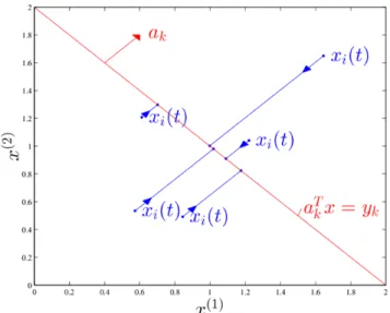
Figure 3.1: Illustration of the idea behind algorithm (3.5).
xi(t) is from satisfying (3.3). Thus, if node i updates xi(t) in such a way that
V(xi(t)) asymptotically decreases to zero, xi(t) would asymptotically satisfy
(3.3). Motivated by this observation, let us take the time derivative ofV(xi(t))
along the trajectory xi(t):
˙
V(xi(t)) =
∑
k∈Ki
(aTkxi(t)−yk)aTkx˙i(t).
To make ˙V(xi(t))≤0, a simple choice is to let
˙
xi(t) = −αi
∑
k∈Ki
(aTkxi(t)−yk)ak, (3.5)
where αi > 0 is a design parameter. With (3.5), xi(t) is guaranteed to move
in a direction where V(xi(t)) decreases or stays the same, as illustrated in
Figure 3.1 whenn = 2 and|Ki|= 1.
Since the goal is for theN nodes to cooperatively find a solution to (3.2), and since every row ofA and Y is known to at least one node, if we forcexi(t)
of every node i ∈ V to not only asymptotically satisfy (3.3), but also achieve a consensus, the consensus value would be a solution to (3.2). In view of this
and the basic idea from continuous-time distributed consensus [1, 7], we add to (3.5) a “consensus” term to arrive at a continuous-time distributed algorithm
˙ xi(t) = −αi ∑ k∈Ki (aTkxi(t)−yk)ak− ∑ j∈Ni β{i,j}(xi(t)−xj(t)), ∀i∈ V, ∀t∈[0,∞), (3.6) where β{i,j} >0 ∀{i, j} ∈ E are also design parameters.
To facilitate its analysis in the next section, note that algorithm (3.6) can be expressed in a matrix form as follows:
˙
x(t) =−(P+L)x(t) +q, (3.7) where x(t) ∈ RnN is a column vector formed by stacking the N x
i(t)’s, while P∈RnN×nN, L∈RnN×nN, and q∈RnN are given by
P= α1 ∑ k∈K1aka T k 0 α2 ∑ k∈K2aka T k . .. 0 αN ∑ k∈KN aka T k , L=Lβ⊗In, q= α1 ∑ k∈K1ykak α2 ∑ k∈K2ykak .. . αN ∑ k∈KNykak ,
where⊗denotes the Kronecker product,Ip ∈Rp×p denotes the identity matrix,
and Lβ = [Lij] ∈ RN×N is a weighted Laplacian matrix of G with Lii =
∑
j∈Niβ{i,j}, Lij =−β{i,j} if {i, j} ∈ E, and Lij = 0 ifi≠ j and {i, j}∈ E/ .
3.4 Algorithm Analysis
In this section, we show that algorithm (3.6) or equivalently (3.7) has several appealing properties, which are reflected in three main results. First,
we show that regardless of its initial conditionx(0), the statex(t) is guaranteed to converge exponentially fast to a point x∗ that depends on x(0) as well as the graph G and problem (3.2). Second, we show that when the solution set of (3.2) is not empty, all the xi(t)’s are guaranteed to converge exponentially
fast to the same point x∗ in the solution set. Finally, we show that when the solution set is empty, at least one node in the graphG is able to asymptotically detect that.
To present the first main result, let
S ={x∈RnN : (P+L)x=q} ⊂RnN
be the set of equilibrium points of (3.7). In addition, since P+L is symmetric positive semidefinite, let itsnN real eigenvalues be denoted as
0 =λ1 =λ2 =· · ·=λr < λr+1 ≤λr+2 ≤ · · · ≤λnN,
where 0 ≤ r ≤ nN, and its corresponding nN orthogonal eigenvectors be denoted as u1, u2, . . . , unN ∈RnN. Moreover, let
Λ = diag(λr+1, λr+2, . . . , λnN)∈R(nN−r)×(nN−r), U=[u1 u2 · · · unN
]
∈RnN×nN
.
Furthermore, let ∥ · ∥ denote the Euclidean norm and both 0p ∈ Rp×p and
0p×q ∈Rp×q be the all-zero matrices, which we will write as 0 whenever there
is no confusion in their sizes.
With these notations, the first main result can be stated as follows:
Theorem 3.1. For every x(0) ∈RnN, there exists a unique x∗ ∈ S such that