San Jose State University
SJSU ScholarWorks
Master's Projects Master's Theses and Graduate Research
Spring 5-22-2019
On Adversarial Attacks on Deep Learning Models
Nag ManiSan Jose State University
Follow this and additional works at:https://scholarworks.sjsu.edu/etd_projects Part of theArtificial Intelligence and Robotics Commons
This Master's Project is brought to you for free and open access by the Master's Theses and Graduate Research at SJSU ScholarWorks. It has been accepted for inclusion in Master's Projects by an authorized administrator of SJSU ScholarWorks. For more information, please contact
Recommended Citation
Mani, Nag, "On Adversarial Attacks on Deep Learning Models" (2019).Master's Projects. 742. DOI: https://doi.org/10.31979/etd.49ee-sknc
On Adversarial Attacks on Deep
Learning Models
By: Nag Mani
Advisor: Melody Moh
CS 298 Report
Department of Computer Science
San Jose State University
San Jose, CA, U.S.A.
© 2019
Nag Mani
Approved by the Designated Project Committee of Project Titled
On Adversarial Attacks on Deep Learning Models
By
Nag Mani
THE DEPARTMENT OF COMPUTER SCIENCE
SAN JOSE STATE UNIVERSITY
April 2019
Dr. Melody Moh
Department of Computer Science, SJSU
Dr. Teng Moh
Department of Computer Science, SJSU
Dr. Chris Pollett
Department of Computer Science, SJSU
ABSTRACT
With recent advancements in the field of artificial intelligence, deep learning has created a niche in the technology space and is being actively used in autonomous and IoT systems globally. Unfortunately, these deep learning models have become susceptible to adversarial attacks which can severely impact their integrity. Research has shown that many state-of-the-art models are vulnerable to attacks by well-crafted adversarial examples. These adversarial examples are perturbed versions of clean data which have small amount of noise added to them. These adversarial samples are imperceptible to the human eye but can easily fool the targeted model. The exposed vulnerabilities of these models raise the question of their usability in safety-critical real-world applications such as autonomous driving and applications in the field of medicine. In this work, I have documented the effectiveness of six different gradient based adversarial attacks on ResNet image recognition model. Defending against these adversaries is a difficult problem and adversarial retraining has been one of the widely used defense technique. Adversarial retraining aims at training a more robust model that is capable of handling the adversarial examples attack proactively. I demonstrate the limitations of the traditional adversarial retraining technique which is effective against some adversaries but fails against more sophisticated attacks. I present a new ensemble defense strategy using adversarial retraining technique which is capable of withstanding six adversarial attacks on cifar10 dataset with accuracy greater than 89.31% and as high as 96.24%.
ACKNOWLEDGEMENT
I would like to extend my heartfelt gratitude to Dr. Melody Moh for being my advisor and one of my first professors at San Jose State University. I am deeply thankful to you for guiding me throughout the project and helping me understand and perform the right experiments.
I am very grateful to Dr. Teng Moh, for taking time out of his busy schedule to help me with my project. His expertise in the field of machine learning and deep learning helped me in understanding some of the difficult concepts of deep learning and eventually completing my project.
I would also like to thank Dr. Chris Pollett for being on my committee. The knowledge I gained from his class on advanced data structures and algorithms helped in analyzing some of the complex algorithms for my project. I am very grateful for his support in my time as a graduate student.
Finally, I would like to thank my family for continually supporting me through graduate school and allowing me the opportunity to pursue a degree in computer science. They have always been there for me and provided me with their emotional support and constant encouragement.
TABLE OF CONTENTS
ABSTRACT ... 4 ACRONYMS ... 7 LIST OF FIGURES ... 8 LIST OF TABLES ... 9 CHAPTER 1. INTRODUCTION ... 10CHAPTER 2. BACKGROUND AND RELATED WORK ... 13
CHAPTER 3. ADVERSARIAL EXAMPLES GENERATION ALGORITHMS ... 14
3.1Fast Gradient Sign Method (FGSM) ... 15
3.2Basic Iterative Method (BIM) ... 16
3.3Iterative Least-Likely Class Method (ILLC) ... 16
3.4DeepFool ... 17
3.5Carlini & Wagner L2 Attack (CWL2)... 17
3.6Carlini & Wagner L infinity Attack (CWL∞) ... 18
CHAPTER 4. DEFENDING THE MODELS ... 19
4.1Challenges of Securing Deep Learning Models ... 19
4.2Adversarial Retraining ... 21 4.3Proposed Solution ... 21 CHAPTER 5. RESULTS ... 23 5.1Experiment Setting ... 23 5.2Implementation Details ... 24 5.3Adversarial Attacks ... 25
5.4Adversarial Retraining: One Model Defense ... 26
5.5Adversarial Retraining: Ensemble Defense ... 27
CHAPTER 6. CONCLUSION AND FUTURE WORK ... 32
ACRONYMS
FGSM:
Fast Gradient Sign Method
BIM:
Basic Iterative Method
ILLC:
Iterative Least-Likely Method
CWL
2:
Carlini-Wagner L2
LIST OF FIGURES
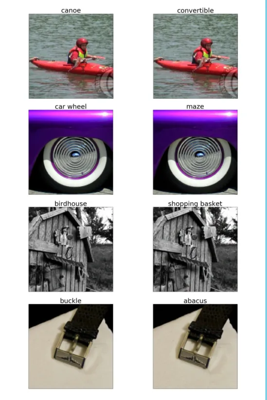
Figure 1: Clean (left) vs adversarial (right) images generated using CWL2 attack ... 12
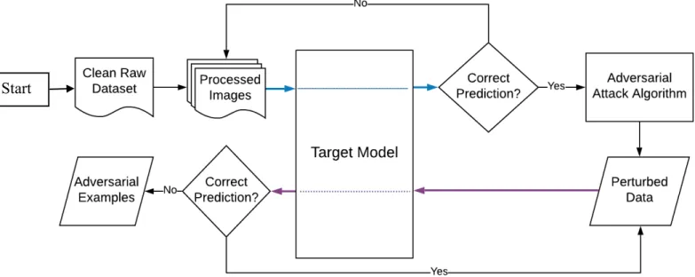
Figure 2: The adversarial examples generation process ... 14
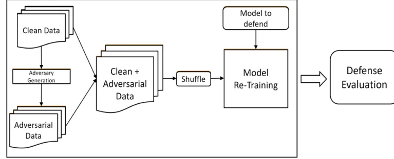
Figure 3: Adversarial retraining process ... 20
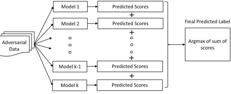
Figure 4: Ensemble adversarial retraining prediction process ... 21
Figure 5: Architecture of one residual block ... 23
Figure 6: ResNet model with 34 residual blocks ... 24
Figure 7: Model accuracy under adversarial examples attack ... 26
Figure 8: Comparative analysis of single model adversarial retraining defense ... 27
Figure 9: Ensemble Adversarial retraining defense results ... 29
Figure 10: Comparative analysis of four model ensembles ... 29
LIST OF TABLES
Table I: Accuracy of six adversarial retrained models ...26
CHAPTER 1. INTRODUCTION
Global research in academia and industry has promoted the adoption of deep learning applications in every aspect of life. From smart home devices like Amazon echo, Google Home and Facebook portal to industrial applications like deliveries by drone, warehouse automation, medical imaging and self-driving vehicles. The inception of these devices in both personal and industrial setting has been accelerated by the advancements in the field of deep learning. Transforming perception into smart responses/action in real time is possible only due to faster and more accurate image recognition models. For instance, smartphones use face detection and recognition to authenticate the correct user. Tesla uses deep learning to design self-driving features such as object detection, semantic segmentation, lane detection, pedestrian detection, traffic sign recognition, etc., to help it make smart decisions in real-time situations. Smart surveillance security cameras are equipped with face and activity recognition which identify and record any abnormal activity or entry.
However, with the wide-scale adoption of IoT devices, the systems are exposed to a multitude of vulnerabilities. One such vulnerability is adversarial examples. These adversarial examples are carefully crafted inputs, aimed at fooling the model and bringing down the model’s accuracy and real-world performance. These attacks are not easy to detect as they are usually imperceptible to humans, yet they can easily degrade the model’s accuracy. The adversaries are asymmetric in nature and are created in specific ways to compromise the integrity of deep learning models. These have posed major risks in implementing deep learning in safety-critical applications, such as home security, medical imaging, and autonomous vehicles.
In this work, I use multiple gradient-based attacks to showcase their effectiveness against the target model. Defense against these attacks has been a well-researched topic and previous work on the topic of adversarial retraining shows its effectiveness against different gradient based attacks [12]. The proposed approach does add some robustness to the model, yet, the decrease in accuracy is more than 25% in the case of adversarial attacks. This is a significant number when considering the
application of these models in safety-critical environments. I have explored the same idea of adversarial retraining to build more resilient models that can withstand adversarial attacks with high confidence. The main contribution of this work is as follows:
• I provided experimental results of six different gradient-based adversarial attacks, including FGSM, BIM, ILLC, DeepFool, Carlini-Wagner L2 and L∞, on ResNet34 model
using cifar10 dataset.
• In order to defend the target model against the attacks, I demonstrate that the previously proposed adversarial retraining technique, [10], has limited effectiveness and does not provide transferable security against more sophisticated attacks.
• I proposed that adversarial retraining technique coupled with our ensemble method is capable of withstanding even sophisticated attacks like Carlini-Wagner attacks [4], achieving model accuracy with minimum of 89.31%, and up to 96.24% for DeepFool attack.
The rest of the work is structured as follows: In Section II, I discuss in brief about the background of our topic and some previous related work. Next, in Section III, I review the set of six gradient-based attacks used for our experiment. Section IV describes the details of our defense architecture which encompasses the adversarial retraining technique coupled with the ensemble approach to perform classification. Finally, Section V describes the experimentation results which is followed by future research direction and conclusion.
Figure 1: Clean (left) vs adversarial (right) images generated using CWL2 attack
CHAPTER 2. BACKGROUND AND RELATED WORK
Though adversarial attacks have been common for a couple of decades, their applications were limited to conventional machine learning methods. For example, variable length of extra padding bits at the end of malware to mask its signature [1], defeating spam filters by appending additional text at end of spam messages are few of the many adversarial attacks which were used against machine learning methods [2].
The idea of adversarial examples attacks which work as a game between an adversary and a machine learning model was first proposed back in 2004 [5]. The approach for attack and defense of the adversarial samples was to play an iterative game which prepared the adversarial examples in an incremental manner. The gradient-based approach was used for the first time to construct adversarial samples back in 2010 [2]. They experimented with multiple models ranging from linear regression, SVM to neural networks. Existence of such adversarial examples for neural networks was shown for the first time back in 2014, where Szegedy researched over the peculiar behavior of neural networks on exposure to such attacks [18].
To counter these adversaries, several defense techniques have been researched upon so far. Adversarial retraining and defensive distillation are some of the widely researched topics. Adversarial retraining involves retraining the target model with adversaries to make it robust against adversarial examples [6, 7, 10]. Defensive distillation works on the idea of a teacher and a student model where soft predictions from the teacher model are used along with the input for making predictions from the student model [16]. However, all proposed defenses have some limitations and have proven to not work against some or more types of adversaries.
CHAPTER 3. ADVERSARIAL EXAMPLES GENERATION
ssssssssssssssssssssssss sss
ALGORITHMS
Figure 2: The adversarial examples generation process
The general concept of adversarial examples, in the context of deep learning, can be represented in form of an optimization problem where the aim is to minimize the objective function that constructs the adversarial examples while keeping it as close as possible to a genuine input. This adversarial example is almost imperceptible to the human eye but can fool the deep learning model. This concept can be summarized in the form of the following equation:
𝐺𝐺𝐺𝐺𝐺𝐺𝐺𝐺𝐺𝐺 ∶ 𝑓𝑓(𝑥𝑥)→ 𝑦𝑦 𝑤𝑤ℎ𝐺𝐺𝑒𝑒𝐺𝐺,𝑥𝑥 ∈[0,1]𝐺𝐺𝑖𝑖𝑡𝑡ℎ𝐺𝐺𝐺𝐺𝐺𝐺𝑖𝑖𝑖𝑖𝑡𝑡, 𝑦𝑦 ∈{𝑦𝑦1,𝑦𝑦2,𝑦𝑦3, … ,𝑦𝑦𝑘𝑘} 𝑎𝑎𝑒𝑒𝐺𝐺𝑡𝑡ℎ𝐺𝐺𝑘𝑘𝑜𝑜𝑖𝑖𝑡𝑡𝑜𝑜𝑜𝑜𝑜𝑜𝐺𝐺𝑙𝑙𝑎𝑎𝑙𝑙𝐺𝐺𝑙𝑙𝑖𝑖 𝐿𝐿𝐺𝐺𝑡𝑡𝑓𝑓�𝑥𝑥𝑗𝑗�=𝑦𝑦𝑗𝑗 𝑒𝑒=��𝑥𝑥𝑗𝑗− 𝑥𝑥𝑗𝑗’�� 𝑖𝑖𝑖𝑖𝑜𝑜ℎ𝑡𝑡ℎ𝑎𝑎𝑡𝑡 0 <𝑒𝑒< 𝜖𝜖 𝑎𝑎𝐺𝐺𝑎𝑎𝑥𝑥𝑗𝑗′ ∈[0,1] 𝑂𝑂𝑙𝑙𝑂𝑂𝐺𝐺𝑜𝑜𝑡𝑡𝐺𝐺𝐺𝐺𝐺𝐺𝐺𝐺𝑖𝑖𝑡𝑡𝑜𝑜𝑜𝑜𝐺𝐺𝐺𝐺𝐺𝐺𝑜𝑜𝐺𝐺𝑚𝑚𝐺𝐺 |𝑒𝑒| ∴ 𝑓𝑓�𝑥𝑥𝑗𝑗′�=𝑦𝑦𝑗𝑗′𝑎𝑎𝐺𝐺𝑎𝑎𝑦𝑦𝑗𝑗≠ 𝑦𝑦𝑗𝑗′
Considering an example of image classification where the images are made up of normalized 𝑥𝑥
pixels and belong to k different categories. 𝑓𝑓(𝑥𝑥)→ 𝑦𝑦 is the function which represents the deep neural Start
network which correctly classifies a sample input image 𝑥𝑥𝑗𝑗 as 𝑦𝑦𝑗𝑗 category. The objective is to create a
new input 𝑥𝑥𝑗𝑗’ which is like 𝑥𝑥𝑗𝑗. Distance measure can be used to quantify the closeness of the two
images which is denoted by 𝑒𝑒. The new image 𝑥𝑥𝑗𝑗’ is constructed by solving the optimization problem
of finding out the minimum value of 𝑒𝑒 which is lower bounded by 0 and upper bounded by a constant
𝜖𝜖. This 𝜖𝜖 controls the overall structural and geometric composition of the synthetic image. A successfully constructed 𝑥𝑥𝑗𝑗’ should be able to produce an output of 𝑓𝑓�𝑥𝑥𝑗𝑗′� as 𝑦𝑦𝑗𝑗′ which is not the
correct result. For a human, the adversarial sample 𝑥𝑥𝑗𝑗′ is still like the original sample 𝑥𝑥𝑗𝑗. Hence a
robust neural network should also classify it as 𝑦𝑦𝑗𝑗, but it fails in doing so [14]. This describes a
successful creation of an adversarial example and a demonstration of how a simple attack can look like in real world.
The architecture for generating such adversarial examples is shown in Figure 2. For our experiment, I selected six different gradient-based attack algorithms briefly described as follows:
3.1 Fast Gradient Sign Method (FGSM)
For many problems, the precision of an individual input feature is limited. Due to this, a classifier can classify an input x and its adversarial example 𝑥𝑥�=𝑥𝑥+𝜂𝜂 to the same class if 𝜂𝜂 is smaller than the precision of the features. Let us consider the following for weight w and the adversarial example 𝑥𝑥� :
𝑤𝑤𝑇𝑇𝑥𝑥�=𝑤𝑤𝑇𝑇𝑥𝑥+𝑤𝑤𝑇𝑇𝜂𝜂 (1)
The adversarial perturbation in equation 1 makes the activation grow by 𝑤𝑤𝑇𝑇𝜂𝜂. The maximum value
of perturbation (||𝜂𝜂 ||∞) does not change with the increase in the number of dimensions. But, if the
weight vector w has n dimensions and the average magnitude of the weight vector is m, then the activation will grow linearly with 𝜖𝜖𝐺𝐺𝑜𝑜. For higher dimensions, an infinitesimal number of small
hypothesize that it is easy to create adversarial examples for inputs with high dimensions. They also hypothesize that neural networks use linear techniques for faster optimization and hence are prone to linear adversarial attacks.
𝜂𝜂 =𝜖𝜖 ∗ 𝑖𝑖𝐺𝐺𝑠𝑠𝐺𝐺�∇x 𝐽𝐽(𝜃𝜃,𝑥𝑥,𝑦𝑦)� (2)
Here, 𝜃𝜃is the parameter of the model, x is the normal input to the model, y is the target output for the input, and 𝐽𝐽(𝜃𝜃,𝑥𝑥,𝑦𝑦) is the cost function for the model. The gradient of the cost function ∇𝑥𝑥 with
respect to the input is calculated. 𝜖𝜖 is used to control the amplitude of the perturbation.
3.2
Basic Iterative Method (BIM)
Extending the logic of FGSM, [9] demonstrated with the use of a smartphone how adversarial examples can fool a deep learning model in real life example. They proposed the algorithm BIM that created samples in an iterative manner with small step size. The algorithm clipped the pixel values of intermediate results whenever the values exceeded the maximum perturbation threshold of ϵ.
𝑥𝑥0𝑎𝑎𝑎𝑎𝑎𝑎 =𝑥𝑥, 𝑥𝑥𝑛𝑛+1𝑎𝑎𝑎𝑎𝑎𝑎 = 𝐶𝐶𝑙𝑙𝐺𝐺𝑖𝑖𝑥𝑥,𝜖𝜖{𝑥𝑥𝑛𝑛𝑎𝑎𝑎𝑎𝑎𝑎 +𝛼𝛼𝑖𝑖𝐺𝐺𝑠𝑠𝐺𝐺(𝛻𝛻𝑥𝑥 𝐽𝐽(𝑥𝑥𝑛𝑛𝑎𝑎𝑎𝑎𝑎𝑎,𝑦𝑦𝑡𝑡𝑡𝑡𝑡𝑡𝑡𝑡))} 𝑤𝑤ℎ𝐺𝐺𝑒𝑒𝐺𝐺,𝑥𝑥:𝑙𝑙𝐺𝐺𝐺𝐺𝐺𝐺𝑠𝑠𝐺𝐺𝐺𝐺𝐺𝐺𝑖𝑖𝑖𝑖𝑡𝑡 𝑥𝑥𝑛𝑛𝑎𝑎𝑎𝑎𝑎𝑎:𝐺𝐺𝑡𝑡ℎ𝑎𝑎𝑎𝑎𝐺𝐺𝐺𝐺𝑒𝑒𝑖𝑖𝑎𝑎𝑒𝑒𝐺𝐺𝑎𝑎𝑙𝑙𝑖𝑖𝑎𝑎𝑜𝑜𝑖𝑖𝑙𝑙𝐺𝐺 𝛼𝛼:𝑖𝑖𝑡𝑡𝐺𝐺𝑖𝑖𝑖𝑖𝐺𝐺𝑚𝑚𝐺𝐺 𝐶𝐶𝑙𝑙𝐺𝐺𝑖𝑖𝑥𝑥,𝜖𝜖:𝐶𝐶𝑙𝑙𝐺𝐺𝑖𝑖𝐺𝐺𝑎𝑎𝑙𝑙𝑖𝑖𝐺𝐺𝑖𝑖𝑤𝑤ℎ𝐺𝐺𝐺𝐺𝑥𝑥𝑎𝑎𝑎𝑎𝑎𝑎 >𝜖𝜖,𝑖𝑖.𝑡𝑡. 𝜖𝜖 > 0
The final adversarial examples were generated after multiple iterations of the algorithm.
3.3 Iterative Least-Likely Class Method (ILLC)
Along with BIM, [9] also proposed an algorithm to attack the model by tricking the model into selecting the least-likely class of a prediction to be its final result. The argument behind this attack was to create a more interesting attack where the adversarial sample was able to trigger a completely unrelated and absurd output.
𝑥𝑥0𝑎𝑎𝑎𝑎𝑎𝑎 =𝑥𝑥, 𝑥𝑥𝑛𝑛+1𝑎𝑎𝑎𝑎𝑎𝑎 = 𝐶𝐶𝑙𝑙𝐺𝐺𝑖𝑖𝑥𝑥,𝜖𝜖{𝑥𝑥𝑛𝑛𝑎𝑎𝑎𝑎𝑎𝑎− 𝛼𝛼𝑖𝑖𝐺𝐺𝑠𝑠𝐺𝐺( 𝛻𝛻𝑥𝑥 𝐽𝐽(𝑥𝑥𝑛𝑛𝑎𝑎𝑎𝑎𝑎𝑎,𝑦𝑦𝐿𝐿𝐿𝐿))} 𝑤𝑤ℎ𝐺𝐺𝑒𝑒𝐺𝐺,𝑥𝑥:𝑙𝑙𝐺𝐺𝐺𝐺𝐺𝐺𝑠𝑠𝐺𝐺𝐺𝐺𝐺𝐺𝑖𝑖𝑖𝑖𝑡𝑡 𝑦𝑦𝐿𝐿𝐿𝐿:𝑙𝑙𝑎𝑎𝑙𝑙𝐺𝐺𝑙𝑙𝑜𝑜𝑓𝑓𝑙𝑙𝐺𝐺𝑎𝑎𝑖𝑖𝑡𝑡𝑙𝑙𝐺𝐺𝑘𝑘𝐺𝐺𝑙𝑙𝑦𝑦𝑜𝑜𝑙𝑙𝑎𝑎𝑖𝑖𝑖𝑖 𝑥𝑥𝑛𝑛𝑎𝑎𝑎𝑎𝑎𝑎:𝐺𝐺𝑡𝑡ℎ𝑎𝑎𝑎𝑎𝐺𝐺𝐺𝐺𝑒𝑒𝑖𝑖𝑎𝑎𝑒𝑒𝐺𝐺𝑎𝑎𝑙𝑙𝑖𝑖𝑎𝑎𝑜𝑜𝑖𝑖𝑙𝑙𝐺𝐺 𝛼𝛼:𝑖𝑖𝑡𝑡𝐺𝐺𝑖𝑖𝑖𝑖𝐺𝐺𝑚𝑚𝐺𝐺 𝐶𝐶𝑙𝑙𝐺𝐺𝑖𝑖𝐺𝐺𝑎𝑎𝑙𝑙𝑖𝑖𝐺𝐺𝑖𝑖𝑤𝑤ℎ𝐺𝐺𝐺𝐺𝑥𝑥𝑎𝑎𝑎𝑎𝑎𝑎 >𝜖𝜖,𝑖𝑖.𝑡𝑡. 𝜖𝜖 > 0
3.4 DeepFool
DeepFool is a method to generate minimal perturbations which is sufficient to mislead the model using iterative linearization approach [13]. Starting with binary classification problem with affine classifiers: 𝑓𝑓(𝑥𝑥) =𝑤𝑤𝑇𝑇𝑥𝑥+𝑙𝑙, the authors assumed that neural networks are linear in nature and each
class is separated by a hyperplane from another. Also, to take in account the non-linearity of neural networks, the approach performs the same steps in iterative manner until an adversary is created. They proved that it is possible to create an adversarial example by using L2 norm in an iterative
manner until the 𝑖𝑖𝐺𝐺𝑠𝑠𝐺𝐺�𝑓𝑓(𝑥𝑥)� ≠ 𝑖𝑖𝐺𝐺𝑠𝑠𝐺𝐺(𝑓𝑓(𝑥𝑥+𝑒𝑒)) where r is the minimum perturbation required. They extended the algorithm to multi class classification and claimed that this approach works with L∞
norm as well. DeepFool was able to create adversarial samples by using smaller perturbations, compared to [9], the average perturbations were five times less. DeepFool is considered as one the more sophisticated attacks and readers can refer to the original work for in depth knowledge [13].
3.5 Carlini & Wagner L
2Attack (CWL
2)
Wagner, challenged the claim by introducing new attack methodology which was successful against both un-distilled and distilled models. In their approach, logits-based loss function was used instead of the softmax cross entropy loss and the target variable was transposed to the argtanh space which helped in solving the problem using modern solvers such as Adam. The approach also used binary search techniques to find the optimal coefficient which balanced the trade-off between prediction and the distance measure. Using the CWL2 attack, they were able to construct more successful adversarial
examples with smaller perturbations.
3.6 Carlini & Wagner L infinity Attack (CWL
∞)
CWL∞ attack follows the same concept of CWL2 but uses an L∞ distance measure instead of L2
distance. CWL∞ attack is more difficult to optimize when compared to L2 attack since it penalizes
only the maximum term. To address the problem, Carlini & Wagner replaced the L2 term in the
objective function with a penalty value which started with 1 but decreased monotonically in each iteration of the algorithm [4].
Finally, L∞ attack is an iterative algorithm which only penalizes the largest perturbation value and
CHAPTER 4. DEFENDING THE MODELS
4.1 Challenges of Securing Deep Learning Models
The existence of adversarial examples that can trick a deep learning model model into performing poorly is an intriguing concept. It is an open topic of research which is of interest for both attackers and researchers who intend to make resilient deep learning models. But, due to the intrinsic nature of deep neural networks, it has not yet been conclusively proven why such samples exist. And, no universal detection or defense mechanism exists that can protect models from any attack. Based on these facts, there are few challenges pertaining to the adversarial examples that currently restrict the researcher community to make better attacks or defense mechanisms. In this section, the authors discuss few of the factors which offer challenges towards defending against adversarial examples.
In 2014, it was found that adversarial examples created from one dataset were able to attack the same deep neural network trained using a different dataset [18]. This was an interesting observation because it hints at the transferable nature of the adversarial examples attack. Later [15], experimented with adversarial examples that were constructed using one deep neural network architecture to attack a different neural network architecture. The results confirmed the transferability property of the adversarial examples. It also empowered the attackers to attack systems with limited or no knowledge using adversarial examples trained on a different model, [11], further explored this characteristic of adversarial examples and proposed that non-targeted attacks are more transferable compared to the targeted attacks.
The question of why adversarial examples exist is an open topic of research. One possible explanation is that exhaustively covering all possible test cases and corner cases would make models
Figure 3: Adversarial retraining process
For linear models that take inputs with high dimensions, the chances of creating adversarial examples become infinitesimal. Even slight changes to the input can result in adversarial examples that the model had not seen before. Reference [6], pointed out that this issue is not limited to just neural networks but other linear models as well.
No universal method exists to defend against adversarial attacks; all attacks and defense are application specific and most of them are based on some specific characteristic of neural networks. Though there is some research that claims to provide universal security, but they have failed, given a small change in attack strategy [3]. Hence as of today, it is not possible to have a 100% secure deep neural network which can resist any adversarial example attack.
Though there is no conclusive explanation for the existence of adversarial examples till now, linearity within model architecture is suspected to be one of the reasons [6]. The high dimensionality of the problem adds to the complexity and even a slight perturbation in the input space can possibly result in an adversary. Theoretically, it is possible to prepare all possible adversaries from input space and then use it to train a robust model which will be immune to adversarial attacks [17]. But such an approach is not feasible to implement, hence alternate defense strategies needs to be explored.
Figure 4: Ensemble adversarial retraining prediction process
4.2 Adversarial Retraining
Adversarial retraining is one of the defense techniques against adversarial examples which uses the adversarial examples for retraining with the objective of building more robust models [6, 7, 10]. Most of the previous work focuses on using FGSM adversaries for adversarial retraining and have shown some promising results on MNIST dataset [12]. But, the problem with such adversaries is that it does not perform well against other types of attacks such as BIM. I extended the same idea of adversarial retraining using adversaries from six different attack models and found out that the problem is not restricted to models retrained with FGSM adversaries. All the six different retrained models did not perform well against one or more of the adversaries.
4.3 Proposed Solution
To create a strong defense strategy, I choose to implement six different gradient-based attack algorithms which included more sophisticated attacks such as ILLC, BIM, DeepFool and
Carlini-constructed from each input batch of clean images and were appended to the input batch which doubled the batch size for each iteration. Hence while retraining each batch contained clean images and their adversarial counterpart. The target model was used for retraining with no transformation in its architecture and with categorical cross entropy loss function. The above described process flow of adversarial retraining is presented in Figure 3.
Each of six retrained models either maintained or improved upon their prediction accuracy of clean images. Upon analysis of the model performance on other adversaries, it was observed that the model trained with FGSM was able to defend against adversaries generated by the ILLC method with an accuracy of 86%. The model retrained with BIM adversaries was able to defend the model against FGSM and ILLC adversaries even more than it could from itself. Similar trends were observed with respect to DeepFool and Carlini-Wagner adversaries. These experiments proved that models retrained using one of the adversaries cannot defend against all but some of the other kind of attacks.
Any single retrained model is not enough to provide substantial defense against all the six adversaries. By using an ensemble of these models, I could achieve better accuracy while encountering adversarial examples attack. The ensemble adversarial defense technique uses four out of the six retrained models to construct a highly robust defense architecture which can withstand even Carlini-Wagner attack with a minimum accuracy of 89.31%. To generate the final prediction from the ensemble of models, I sum up the class-wise individual predicted scores from each model. As depicted in Figure 4, from this final predicted score I select the argmax of the vector to obtain the final prediction category. This strategy is better than hard majority voting technique since it exploits the increased confidence of retrained models for identifying the correct class.
CHAPTER 5. RESULTS
The set of experiments for this work includes the implementation of FGSM, BIM, ILLC, DeepFool, Carlini-Wagner L2 and L∞ attacks on ResNet34 model using cifar10 dataset. The attack
effectiveness of these adversaries is analyzed to understand their relative strengths and weaknesses. The objective is to use these adversaries for defending the target model, such that the defense is transferable to other kinds of attacks as well.
5.1
Experiment Setting
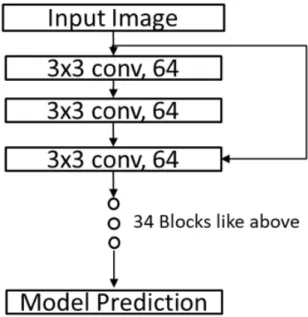
For this experiment, I selected the ResNet model with 34 layers as our target model [8]. The cifar10 dataset was selected because of its size and specification which allowed us to execute such large set of experiments. To implement the attacks and ensemble defense, I used PyTorch framework in python3 and used a computer with the following specifications: Intel i7 processor, 16 GB RAM and 6 GB GPU (GTX 1060). For attack, the model architecture shown in Figure 2 was used to generate adversaries using the target model.
Figure 6: ResNet model with 34 residual blocks
5.2
Implementation Details
This project has been structured in two parts: the first part involves creating adversaries using six adversary generation algorithm and the second part consists of defending the target model from these adversaries. For creating adversaries to evaluate the six types of attacks in first part of the project, I have used the 10000 images from test set of the cifar10 dataset.
The value of epsilon for FGSM attack was set to 0.1, which ensured that the perturbations added to the original image was in the range of [0,0.1]. Similarly, the starting epsilon value for BIM and ILLC attack was set to 0.001 and the number of maximum perturbations were set to 10. For Deep Fool,
CWL2 and CWL∞ attacks number of maximum permissible iterations was set to 10 as well. The loss
function in case of DeepFool was categorical cross entropy and for Carlini-Wagner L2 and L∞
attacks it was argtanh.
In part two of the project, the adversarial retraining strategy used the pre-trained weights of the target model that was trained on clean data. The dataset for retraining was prepared by generating adversarial samples from clean train dataset (50000 images) using the six algorithms from part one and the adversarial samples were shuffled with the clean sample to create a new master dataset
consisting of clean samples and their adversarial counterparts. The model was then retrained using a batch size of 64 and 10 epochs. Loss function was categorical cross entropy and the optimizer used was adadelta. Using the above setup six different retrained models was retrained using the six adversarial algorithms. These six retrained models were used for subsequent experiments pertaining to ensemble strategy. The implementation of the all the attacks and the defense strategy can be found at the following link: https://github.com/mani-nm/Adversarial_Examples
5.3
Adversarial Attacks
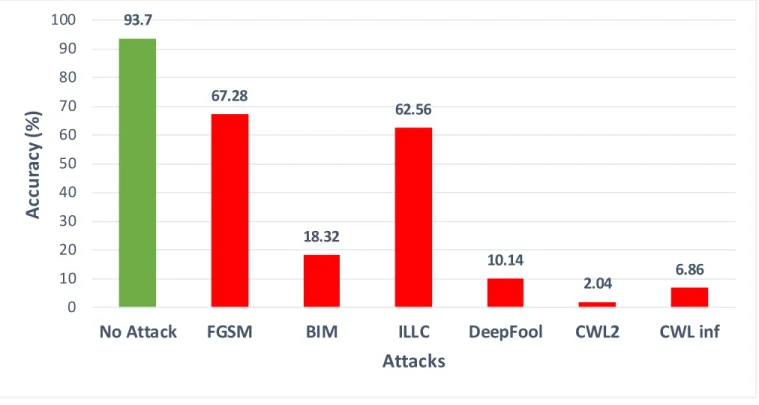
The selected set of adversarial attack algorithms were implemented using the target model: ResNet with 34 layers which had a base accuracy of 93.7% on the test set of clean images. The standard set of 10000 test images from cifar10 was used to create adversaries for the experiment. The results of adversarial examples attack on model accuracies is shown in Figure 5. Target model’s base accuracy is plotted with label “No Attack” and its accuracy under different attacks are plotted thereafter. Among the attacks, FGSM was least lethal with model accuracy maintaining at 67.28% which was followed by ILLC at 62.57% which uses a similar attack signature. Among the stronger attacks: model accuracy dropped to 18.32% for BIM and CWL2 was most effective attack where the model
Figure 7: Model accuracy under adversarial examples attack
5.4
Adversarial Retraining: One Model Defense
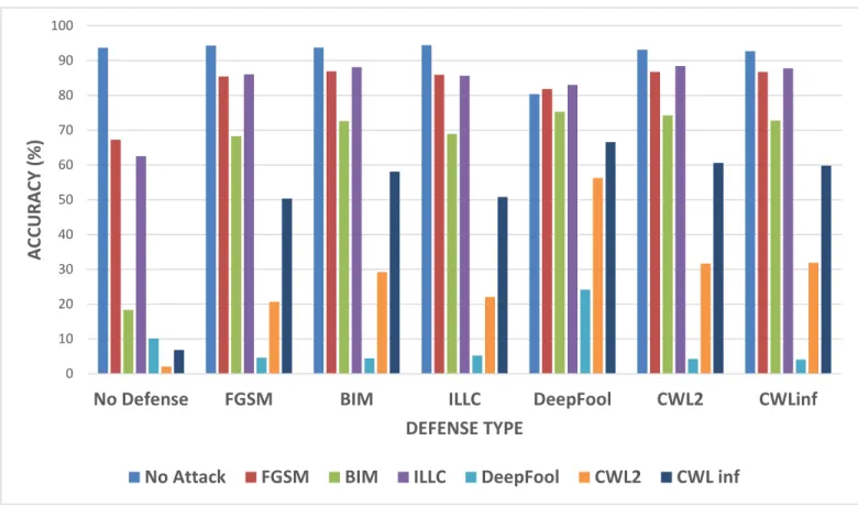
Adversarial retraining was done on the train set of 50000 images from cifar10 using the architecture shown in Figure 3. The pre-trained target model was used for retraining and a static copy of the same model was decoupled and used for producing adversaries as part of the retraining architecture. Base batch size of 64 was used for adversary generation and the generated adversaries were appended to the batch for retraining. Six models were obtained from retraining exercise and their individual effectiveness is presented in Table I, where the bold values highlight the best accuracy for each attack. Each of the retrained models is
Table I: Accuracy of six adversarial retrained models
93.7 67.28 18.32 62.56 10.14 2.04 6.86 0 10 20 30 40 50 60 70 80 90 100
No Attack FGSM BIM ILLC DeepFool CWL2 CWL inf
Accu
ra
cy (
%
)
Attacks
No DefenseAttack Base Accuracy FGSM BIM ILLC DeepFool CWL2 CWLinf
No Attack 93.7 94.34 93.73 94.44 80.36 93.14 92.75 FGSM 67.28 85.43 86.95 85.94 81.84 86.76 86.74 BIM 18.32 68.29 72.61 68.94 75.32 74.26 72.79 ILLC 62.56 86.06 88.09 85.69 83.07 88.46 87.76 DeepFool 10.14 4.59 4.46 5.24 24.22 4.3 4.09 CWL2 2.04 20.69 29.25 22.08 56.29 31.65 31.88 CWL inf 6.86 50.33 58.12 50.82 66.56 60.63 59.81
Figure 8: Comparative analysis of single model adversarial retraining defense
evaluated against all six types of adversaries, to test their robustness. Model retrained with FGSM adversaries improves the base accuracy of the target model when tested on clean images. In general, FGSM, BIM and ILLC can be defended fairly against adversaries by using any of retrained model. There is some improvement in retrained model accuracy in case of DeepFool and Carlini-Wagner attacks as compared to their respective attack effectiveness on the undefended model. But, the improvement is not enough to allow the model to be used confidently in a real-world scenario.
5.5
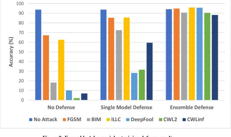
Adversarial Retraining: Ensemble Defense
For our next experiment, I created an ensemble of all the retrained models which were used for predicting instead of a single model. The predicted softmax score from each retrained model was
0 10 20 30 40 50 60 70 80 90 100
No Defense FGSM BIM ILLC DeepFool CWL2 CWLinf
ACCU
RA
CY
(%)
DEFENSE TYPE
model ensemble defense are shown in Figure 6. It gives a better result compared to any single model-based prediction used in adversarial retraining experiment. Even complicated attacks like Carlini-Wagner L∞ could be successfully resisted with an accuracy of 88.2% and ILLC was most confidently
defended with an accuracy of 95.91%.
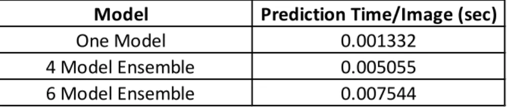
The increased accuracy from the ensemble method comes at the price of performance where the prediction time of six model ensemble is 5.6 times that of the single model prediction time. Given most of the models are used in real-time systems, limiting prediction latency is also one of the key factors. Keeping this in mind, the final set of experiments explored the idea of creating an ensemble of the retrained model that are capable of thwarting an adversarial attack and at the same time do not sacrifice a lot of prediction performance.
I experimented with different combinations of model ensembles and realized that an ensemble of four models out of six gave the best performance and accuracy tradeoff. To identify the ideal set of four models, I experimented with different combinations of retrained models. Groups were created based on the following criteria: nature of attack, attack strength and adversarial retrained model’s accuracy. FGSM and ILLC demonstrated similar levels of attack strength and their respective adversarial retrained model can defend one another.
Figure 9: Ensemble Adversarial retraining defense results 0 10 20 30 40 50 60 70 80 90 100
No Defense Single Model Defense Ensemble Defense
Accu
ra
cy
(%
)
No Attack FGSM BIM ILLC DeepFool CWL2 CWLinf
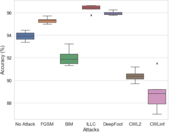
82 84 86 88 90 92 94 96 98 ILLC, BIM, DEEPFOOL, CWL2 FGSM, BIM, DEEPFOOL, CWL2 ILLC, BIM, DEEPFOOL, CWLINF ILLC, BIM, CWL2, CWLINF FGSM, BIM, CWL2, CWLINF BIM, DEEPFOOL, CWL2, CWLINF ACCU RA CY (% ) Recommended
Figure 11: Box-plot of variation of four-model ensemble defense under each attack type
Hence, I pick only one of these two in the ensemble and never both. The challenge with adversarial defense was to identify the right combination of other retrained model which could defend against sophisticated attacks like BIM, DeepFool, CWL2 and CWL∞ attacks. The results of the experiment
are shown in Figure 7, using which I can recommend that an ensemble of FGSM, BIM, CWL2 and
CWL∞ gives the most balanced prediction accuracies against all six kinds of attacks. The spread of
ensemble prediction accuracy for each kind of attack can be analyzed using the box plots in Figure8. FGSM, ILLC and DeepFool attacks are defended with consistency using all the four model ensembles, whereas CWL∞ and BIM do show some spread and appears to perform better with an
ensemble of sophisticated models.
Another interesting observation from this experiment is that all the subsets of the ensembles provide comparable defense against all adversaries when compared to six model ensemble and are 33% faster compared to it, as presented in Table II. Using a different set of four models for ensemble in different prediction rounds can protect the ensemble model against further attacks.
Table II: Defense model prediction time
The results of the experiment show that the ensemble of these four models can be effectively used to defend against all six of the adversaries. The DeepFool attack which was immune to all single defense approach can be defended with an accuracy of 96.24% and CWL2 attack could be defended
with a confidence of 91.2%. Similarly, BIM and CWL∞ attacks can be successfully defended against
with an accuracy of 93.23% and 91.5% respectively. Hence, the ensemble approach can defend the target model with more confidence against most types of gradient-based adversaries.
Model Prediction Time/Image (sec)
One Model 0.001332
4 Model Ensemble 0.005055
CHAPTER 6. CONCLUSION AND FUTURE WORK
Deep Learning has facilitated the application of artificial intelligence in security critical applications by creating highly accurate and precise models. Its vulnerability to adversarial examples, however, has raised serious concerns regarding its full-fledged adoption. In this report, I have discussed the vulnerabilities of deep learning models with respect to adversarial example attacks. Even though some research has been conducted to construct adversarial examples and to defend deep learning models against them, the core idea behind the existence of adversarial examples is still elusive to the research community. Most of the proposed attacks work on a specific model configuration and countermeasures for these are prepared to protect against the corresponding attacks. Carlini & Wagner showcased that the recent existing defense strategies are rigid in structure and can be defeated by using a new loss function in existing attack strategies. Hence, as of now, no universal defense strategy exists for different kinds of adversarial example attacks.
After researching upon the subject, some observations may be derived to guide the future research direction. Firstly, most researchers have chosen to show their work on the MNIST dataset, which is a considerably small and basic dataset. Next, quantifying the robustness of defense must be done against a significant number of attacks which should include both basic and sophisticated attacks. In addition, there exists a need for a standard platform where different attacks can be performed and evaluated on a large scale.
Adversarial examples pose a serious threat to the real-time deployment of deep learning image recognition models. The impact of these attacks can be severe and securing these models against such attacks is of paramount importance. In this work, I selected a set of six strong attacks and demonstrated their effectiveness against state of the art ResNet model. Experimentation with strong attacks is the only way to ensure that strong defense techniques can be explored. I demonstrated that previously proposed adversarial retraining defense technique can only be partially effective and
proposed a new ensemble method which used four different adversarial retrained model to perform model predictions. Results of my experiments show the strengths of the ensemble defense and prove that by using a subset of adversaries, a target model can be defended from some of the unseen attacks.
In my project, I researched and experimented in depth about gradient-based adversaries and for future experimentation attacks other than gradient-based attacks can be explored. Evaluation of my ensemble defense strategy could be evaluated against new types of attacks. Adversarial retraining is one of proactive approaches for defending deep learning models, similar proactive strategies can be researched upon which can increase model’s robustness against such attacks.
Another interesting future work could be to compare the retrained robust models and the original target model to understand the effects the retraining upon the internal weights of the network. Analyzing the differences between the two network weights can shed some light upon the different layers and neurons which adds to the robustness of the retrained network and eventually provides security to the original model.
REFERENCES
[1] A. Madry, A. Makelov, L. Schmidt, D. Tsipras and A. Vladu, "Towards deep learning models resistant to adversarial attacks," arXiv Preprint arXiv:1706.06083, (2017).
[2] A. Kurakin, I. Goodfellow and S. Bengio, "Adversarial machine learning at scale," arXiv Preprint arXiv:1611.01236, (2016).
[3] N. Carlini and D. Wagner, "Towards Evaluating the Robustness of Neural Networks," 2017 IEEE Symposium on Security and Privacy (SP), 2017, pp. 39-57.
[4] M. Barreno, B. Nelson, A.D. Joseph and J.D. Tygar, "The security of machine learning," Machine Learning, 81, 121-148 (2010).
[5] B. Biggio, G. Fumera and F. Roli, "Multiple classifier systems for robust classifier design in adversarial environments," International Journal of Machine Learning and Cybernetics, 1, 27-41 (2010).
[6] N. Dalvi, P. Domingos, S. Sanghai and D. Verma, "Adversarial Classification," Proceedings of the Tenth ACM SIGKDD International Conference on Knowledge Discovery and Data Mining, 2004, pp. 99-108.
[7] C. Szegedy, W. Zaremba, I. Sutskever, J. Bruna, D. Erhan, I. Goodfellow and R. Fergus, "Intriguing properties of neural networks," (2013).
[8] S. Gu and L. Rigazio, "Towards deep neural network architectures robust to adversarial examples," arXiv Preprint arXiv:1412.5068, (2014).
[9] I.J. Goodfellow, J. Shlens and C. Szegedy, "Explaining and harnessing adversarial examples," (2014).
[10] N. Papernot, P. McDaniel, X. Wu, S. Jha and A. Swami, "Distillation as a defense to adversarial perturbations against deep neural networks," arXiv Preprint arXiv:1511.04508, (2015).
[11] N. Mani and M. Moh, "Adversarial Attacks and Defense on Deep Learning Models for Big Data and IoT," in Handbook of Research on Cloud Computing and Big Data Applications in IoT, edited by Anonymous (IGI Global2019), pp. 39-66.
[12] A. Kurakin, I. Goodfellow and S. Bengio, "Adversarial examples in the physical world," arXiv Preprint arXiv:1607.02533, (2016).
[13] S. Moosavi-Dezfooli, A. Fawzi and P. Frossard, "Deepfool: A Simple and Accurate Method to Fool Deep Neural Networks," Proceedings of the IEEE Conference on Computer Vision and Pattern Recognition, 2016, pp. 2574-2582.
[14] N. Papernot, P. McDaniel and I. Goodfellow, "Transferability in machine learning: From phenomena to black-box attacks using adversarial samples," arXiv Preprint arXiv:1605.07277, (2016).
[15] Y. Liu, X. Chen, C. Liu and D. Song, "Delving into transferable adversarial examples and black-box attacks," arXiv Preprint arXiv:1611.02770, (2016).
[16] K. Pei, Y. Cao, J. Yang and S. Jana, "Deepxplore: Automated Whitebox Testing of Deep Learning Systems," Proceedings of the 26th Symposium on Operating Systems Principles, 2017, pp. 1-18.
Proceedings of the IEEE Conference on Computer Vision and Pattern Recognition, 2016, pp. 770-778.
[19] A. Madry, A. Makelov, L. Schmidt, D. Tsipras and A. Vladu, "Towards deep learning models resistant to adversarial attacks," arXiv Preprint arXiv:1706.06083, (2017).