DOI:10.1214/16-AOAS926
©Institute of Mathematical Statistics, 2016
A SPATIOTEMPORAL NONPARAMETRIC BAYESIAN MODEL OF MULTI-SUBJECT FMRI DATA
BYLINLINZHANG∗, MICHELEGUINDANI†, FRANCESCOVERSACE‡,
JEFFREYM. ENGELMANN§ ANDMARINA VANNUCCI∗
Rice University∗, MD Anderson Cancer Center†, University of Oklahoma Health Sciences Center‡and MD Anderson Cancer Center§
In this paper we propose a unified, probabilistically coherent framework for the analysis of task-related brain activity in multi-subject fMRI experi-ments. This is distinct from two-stage “group analysis” approaches tradition-ally considered in the fMRI literature, which separate the inference on the individual fMRI time courses from the inference at the population level. In our modeling approach we consider a spatiotemporal linear regression model and specifically account for the between-subjects heterogeneity in neuronal activity via a spatially informed multi-subject nonparametric variable selec-tion prior. For posterior inference, in addiselec-tion to Markov chain Monte Carlo sampling algorithms, we develop suitable variational Bayes algorithms. We show on simulated data that variational Bayes inference achieves satisfac-tory results at more reduced computational costs than using MCMC, allow-ing scalability of our methods. In an application to data collected to assess brain responses to emotional stimuli our method correctly detects activation in visual areas when visual stimuli are presented.
1. Introduction. Functional magnetic resonance imaging (fMRI) is a nonin-vasive neuroimaging technique which measures the blood oxygenation level de-pendent (BOLD) contrast, that is, the difference in magnetization between oxy-genated and deoxyoxy-genated blood arising from changes in regional cerebral blood flow. In a typical task-related fMRI experiment, a subject is presented a set of stim-uli while the whole brain is scanned at multiple time points. Each scan is arranged as a 3D array of volume elements (or “voxels”), and the experiment produces time series of BOLD responses acquired at each voxel.
Common modeling approaches for the analysis of task-related fMRI data rely on the linear model formulation that was first proposed by Friston, Jezzard and Turner(1994) and subsequently investigated by many other authors, particularly for single-subject data; see, for example, Friston et al. (1995, 2002), Lee et al.
(2014), Lindquist (2008), Quirós, Diez and Gamerman (2010), Woolrich et al.
(2004), Worsley and Friston (1995), Zhang et al. (2014), among many others. Many of these models incorporate the complex spatial and temporal correlation
Received May 2015; revised December 2015.
Key words and phrases.Multi-subject fMRI, spatiotemporal linear regression, variable selection priors, variational Bayes.
structure of the fMRI data. Bayesian approaches, in particular, allow flexible mod-eling of spatial and temporal correlations via suitable prior models and can achieve increased signal detection and fewer false positive counts with respect to simpler approaches that do not appropriately account for the spatiotemporal variability of the data; see, for example,Zhang, Guindani and Vannucci(2015) for a review of recent Bayesian models.
While spatiotemporal models have been extensively investigated for single-subject analysis, in multi-single-subject studies two-stage “group analysis” approaches are often adopted as computationally attractive methods where summary estimates of model parameters are obtained at the individual level and then used in a sec-ond stage model at the group/population level [Bowman et al. (2008), Holmes and Friston(1998),Li et al.(2015),Sanyal and Ferreira(2012),Su et al.(2009)]. In contrast, in this paper we propose a unified, single stage and probabilistically coherent Bayesian framework for the analysis of task-related brain activity in multi-subject fMRI experiments. Our model formulation considers a spatiotem-poral linear regression model and specifically accounts for between-subjects het-erogeneity in neuronal activity via a spatially informed multi-subject nonparamet-ric variable selection prior. Bayesian nonparametnonparamet-ric models, especially standard Dirichlet Processes [Ferguson(1973)], have been used successfully in fMRI data analysis, particularly in the context of Gaussian mixture models applied to pro-cessed data (either “contrast” maps or simple z-statistic images), to capture dis-tinct clusters of activations [Jbabdi, Woolrich and Behrens(2009),Johnson et al.
(2013),Kim, Smyth and Stern(2006)]. Also, Hartvig and Jensen(2000) and Xu et al.(2009) model the inter-subject variability in activation locations via Gaussian mixture models that estimate the probability that an individual has an activation at a particular location. In this paper, we leverage on more advanced multi-level Bayesian nonparametric approaches [Teh et al.(2006)] to allow for the separate inferential objectives within and between subjects. In more detail, we employ a hierarchical Dirichlet Process prior construction to induce clustering among vox-els within a subject at one level of the hierarchy and across subjects at the second level. This formulation allows, in particular, to capture spatial correlation among potential activations of distant voxels, within a subject, while simultaneously bor-rowing strength in the estimation of the parameters from subjects with similar activation patterns. In the fMRI literature, capturing statistical dependence among possibly remote neurophysiological events is often viewed as an aspect of “func-tional” connectivity [Friston(1994,2011)]. Furthermore, we take into account the spatial proximity of potential activations within a subject by employing a Markov Random Field (MRF) prior.
A single fMRI experiment can yield hundreds of thousands of high frequency time series for each subject, arising from spatially distinct locations. Clearly, uni-fied approaches, like the one we propose, pose challenges from a computational point of view. In this paper, in addition to a Markov chain Monte Carlo sampling
algorithm for posterior inference, we develop a suitable variational Bayes algo-rithm that does not rely on numerical integration but rather find a suitable ap-proximation of the true posterior density. Variational Bayes methods have been employed successfully in Bayesian models for single-subject fMRI data [Flandin and Penny(2007),Harrison and Green(2010),Penny, Kiebel and Friston(2003),
Penny, Trujillo-Barreto and Friston(2005),Woolrich, Behrens and Smith(2004)]. Typically, these approaches provide good estimates of means, although they tend to underestimate posterior variances and also to poorly estimate the correlation structure of the data [Bishop(2006),Rue, Martino and Chopin(2009)]. In a com-parative study on simulated data, we show that the variational Bayes algorithm achieves robust estimation results at much reduced computational costs, therefore allowing scalability of our methods. Additionally, we demonstrate on synthetic data how our unified, single-stage, multiple-subject modeling approach, with vari-ational Bayes inference, achieves improved estimation performance with respect to two-stage approaches.
We show the practical relevance of the proposed model by presenting an ap-plication to data from a study aimed at assessing brain responses to natural vi-sual scenes. The experiment was conducted at the Department of Behavioral Science at the University of Texas MD Anderson Cancer Center [Versace et al.
(2013)]. During the experiment brain responses from 27 female participants were recorded during the presentation of emotional and neutral images. We show that our method correctly detects activations in a coronal slice covering the occipital cortex. We also show results on a second coronal slice in the frontal areas, where passive viewing of visual stimuli are not expected to lead to increased brain acti-vation.
The rest of the paper is organized as follows: Section 2 introduces the spa-tiotemporal model and the proposed spatially informed multi-subject nonparamet-ric variable selection prior. Section3describes the MCMC and variational Bayes algorithm for posterior inference. In Section4, we carry out a performance com-parison between MCMC and variational Bayes inference using simulated data. We also perform a comparison between our unified, single-stage method and an alter-native two-stage approach. We then analyze the case study data, where we show that our method correctly detects activation of visual areas when visual stimuli are presented. Section5concludes the paper.
2. Multi-subject spatiotemporal model. We describe our proposed multi-subject Bayesian spatiotemporal regression model for fMRI data, which includes correlated errors and a spatially informed variable selection prior.
2.1. Regression model with correlated errors. LetYiν=(Yiν1, . . . , YiνT)T be the T ×1 vector of the BOLD response data at the νth voxel in theith subject,
withi=1, . . . , N, ν=1, . . . , V, and with the symbol(·)T indicating the transpose operation. We model the BOLD time-series response with a general linear model (2.1) Yiν=Xiνβiν+εiν, εiν∼NT(0, iν),
whereXiνis aT ×pcovariate matrix, βiν=(βiν1, . . . , βiνp)T is ap×1 vector of regression coefficients andεiν=(εiν1, . . . , εiνT)T is a T ×1 vector of errors. Without loss of generality, we center the data, and thus do not include the inter-cept term in the model. Linear models of type (2.1) are commonly used in multi-subject fMRI approaches that employ two-stage “group analysis,” where summary estimates of model parameters are obtained at the subject level by fitting the linear model voxel-wise and then used in the second stage model at the group/population level [Bowman et al.(2008),Holmes and Friston(1998),Li et al.(2015),Sanyal and Ferreira(2012),Su et al.(2009)].
Let us consider model (2.1) in the case of a single experimental task or input stimulus (p=1). The vectorXiν models the lapse of time between the stimulus onset and the vascular response, and it is typically obtained as the convolution of the stimulus pattern with a hemodynamic response function (HRF). More specifi-cally, here we use a Poisson HRF [Buxton and Frank(1997),Friston, Jezzard and Turner(1994)] and modelXiνas
(2.2)
t
0 x(s)hλiν(t−s) ds,
withx(s)the known time-dependent stimulus function andhλiν=exp(−λiν)λtiν/ t!, withλiν a subject-specific and voxel-dependent parameter.
The error terms in (2.1) capture temporal correlation in the fMRI data and are typically assumed autocorrelated, accounting for both hardware and subject-related noise [Lee et al. (2014), Penny, Kiebel and Friston (2003), Woolrich et al. (2004)]. Here we write the error covariance matrix in (2.1) asiν(t, s)= [γ (|t−s|)] withγ (h) the autocovariance function of the process generating the data, and then assumeγ (h) to have a fractal behavior of the typeγ (h)∼Ch−α withC a positive constant, 0< α <1 andhlarge. This choice accounts for low-frequency noise which induces slow changes in voxel intensity over time, such as scanner drift, and for physiological noise, due to patient motion, respiration and heartbeat, causing fluctuations in signal across both space and time. In an analysis of single-subject fMRI data,Zhang et al.(2014) show that such a modeling strat-egy improves the deconvolution of the signal and the noise, leading to the detection of more localized, fewer false positive and sparser activations with respect to using autoregressive error structures.
Discrete wavelet transforms (DWT) are often employed in the fMRI literature as a way to decorrelate the data, allowing inference on the model parameters based on the transformed data [Fadili and Bullmore(2002),Jeong, Vannucci and Ko(2013),
computationally advantageous, particularly for the long memory error structure we employ. When applying a DWT to both sides of (2.1), the model transforms into (2.3) Yiν∗ =X∗iνβiν+ε∗iν, ε∗iν∼NT0, iν∗,
whereYiν∗ =W Yiν, Xiν∗ =W Xiν, andε∗iν=W εiν and whereW is an orthogonal T ×T matrix representing the wavelet transform. The wavelet transform reduces the covariance matrix iν∗ to a T ×T diagonal matrix, with diagonal elements, ψiνσimn2 , indicating the variance of the nth wavelet coefficient at the mth scale. We adopt the variance progression formula
(2.4) ψiνσimn2 =ψiν2αiν−m,
withψiνthe innovation variance andαiν∈(0,1)the long memory parameter. This structure encompasses the general fractal process given above, which includes long memory [Wornell and Oppenheim(1992)].
2.2. Spatially informed nonparametric variable selection prior. In model (2.1) the detection of brain voxels that activate in response to the stimulus reduces to a problem of variable selection, that is, the identification of the nonzero βiν, and is achieved, in the Bayesian framework, by imposing a mixture prior, often called a spike-and-slabprior, on the regression coefficients [Kalus, Sämann and Fahrmeir (2014),Lee et al.(2014),Zhang et al.(2014)]. In our model formula-tion, we embed the selection into a clustering framework and effectively define a multi-subject nonparametric variable selection prior with spatially informed selec-tion within each subject. This allows us to specifically account for the between-subjects heterogeneity in neuronal activity. More specifically, we employ a hi-erarchical Dirichlet Process (HDP) prior [Teh et al. (2006)], which implies that the nonzero βiν’s within subject i are drawn from a mixture model and possi-bly shared between subjects. We assume that the number of mixture components is unknown and inferred from the data. The HDP prior construction effectively captures correlation among time-series voxels within and across subjects by in-ducing clustering among voxels within a subject at one level of the hierarchy and between subjects at the second level. This allows, in particular, to capture spatial correlation among potential activations of distant voxels, within a subject while simultaneously borrowing strength in the estimation of the parameters from sub-jects showing similar activation patterns. Furthermore, we take into account the spatial proximity of potential activations within a subject by employing a Markov Random Field (MRF) prior on the selection indicators of the spike-and-slab distri-bution.
In more detail, letγiν be the binary indicator of whether voxel ν in subjecti is active or not, that is, γiν=0 if βiν=0 and γiν=1 otherwise. We impose a spiked HDP prior onβiν, which we define as a spike-and-slab prior where the slab
distribution is modeled by a HDP prior,
βiν|γiν, Gi∼γiνGi+(1−γiν)δ0, Gi|η1, G0∼DP(η1, G0),
(2.5)
G0|η2, P0∼DP(η2, P0), P0=N (0, τ ),
with δ0 a point mass at zero, with τ fixed, η1, η2 the mass parameters and P0 the base measure. With this prior formulation, the subject-specific distribution Gi varies around a population-based distribution G0, which is centered around a known parametric model P0. The mass parameters η1 andη2 control the vari-ability of the distribution of the coefficients at the subject and population lev-els, respectively. The use of a nonparametric prior allows us to leverage on the goodness-of-fit properties of this class of flexible Bayesian priors for density estimation. Both Gi and G0 can be written as a mixture of point masses as Gi=∞k=1πikδφkandG0=
∞
k=1ξkδφk, whereδx indicates a point mass atxand the mixture weights are given, respectively, byπik=πik
k−1
l=1(1−πil), withπik ∼ Beta(η1xik, η1(1−kl ξl)), andξk=ξk
k−1
l (1−ξl), withξk∼Beta(1, η2); see
Sethuraman(1994). The mixture representation highlights the fact thatGi andG0 share common atoms φk∼P0, and thus naturally induce clustering of the βiν’s in (2.5). As a result, the coefficientsβiν’s may be effectively shared across active voxels within a subject as well as between subjects. For computational purposes, it’s often convenient to consider a truncated representation of the mixturesGiand G0, where suitably large finite sums are considered in lieu of the infinite sum representation above [Ishwaran and James(2001)]. In applications where the true number of clusters is generally unknown, it is good practice to set relatively high truncation levels. In this paper, we report results with the within-subject truncation set to 20 and the across-subjects truncation set to 15. Higher truncation levels gave similar results with only a small increase of the computation time.
In order to take into account information on the anatomical structure of the brain, in particular, the correlation between neighboring voxels, we place a Markov Random Field (MRF) prior on the selection parameterγiν,
(2.6) P (γiν|d, e, γik, k∈Niν)∝exp γiν d+e k∈Niν γik ,
with Niν the set of neighboring voxels of voxelν in subjecti. The use of MRF priors has become quite popular in recent years in the Bayesian modeling of fMRI data [Lee et al.(2014),Smith and Fahrmeir(2007),Xia, Liang and Wang(2009),
Zhang et al.(2014)]. The sparsity parameterd∈(−∞,∞)represents the expected prior number of activated voxels. The smoothing parameter e >0 controls the probability of identifying a voxel as active based on the activation of its neigh-boring voxels. Prior (2.6) reduces to an independent Bernoulli with parameter
exp(d)/[1+exp(d)] if a voxel does not have any neighbors. In the applications of this paper we fix the values ofd ande, in particular, following the guidelines of
Zhang et al.(2014).
Finally, we complete our prior model by considering a uniform prior distribu-tion on the delay parameter,λiν∼U(u1, u2). We also impose an Inverse Gamma (IG) prior on the innovation variance parameter,ψiν∼IG(a0, b0), and a Beta dis-tribution on the long memory parameter,αiν∼Beta(a1, b1).
3. Model fitting. We investigate two approaches, a Markov chain Monte Carlo (MCMC) algorithm and a variational Bayes (VB) algorithm for posterior inference. The MCMC algorithm combines Metropolis–Hastings (MH) schemes that use theadd-delete-swapmoves [Savitsky, Vannucci and Sha(2011)] with sam-pling algorithms for hierarchical Dirichlet process (HDP) models that use auxiliary parameters for cluster allocation [Savitsky and Vannucci(2010),Teh et al.(2006)]. To ensure scalability, we also investigate an alternative approach that uses varia-tional Bayes (VB) inference, combining a truncated stick-breaking construction for the hierachical Dirichlet process [Blei and Jordan (2006),Wang, Paisley and Blei(2011)] with the importance sampling procedure ofCarbonetto and Stephens
(2012). In the simulation section, we show how the VB algorithm reduces the computational cost without compromising the accuracy of the estimation.
3.1. Markov chain Monte Carlo algorithm. We briefly describe the updates of the model parameters at a generic iteration. Full details of the posterior distri-butions and our implementation are in the supplementary material [Zhang et al.
(2016)].
• Update β and γ: We update these parameters jointly with a Metropolis– Hastings algorithm. We first selectnsubjects at random using a truncated Pois-son distribution with mean parameterN/2, whereN is the total number of sub-jects, and 0< n≤N. For each of the selected subjects, denoted by subjecti, we perform anadd-delete-swapmove: for theaddmove, we choose at random one voxelν, and change the value of its selection parameterγiνfrom 0 to 1, and si-multaneously update the value of its regression coefficientβiνwith the sampling algorithm for HDP models proposed inTeh et al. (2006); for the deletemove, we change γiν for the randomly chosen voxelν from 1 to 0, and set βiν=0; for the swapstep, we choose two voxels with different activation status, swap their values ofγ, and update the values ofβaccordingly. The proposed move is accepted with probability
min
1,f (Y
∗|βnew, γnew, λ, ψ, α)π(βnew|γnew)π(γnew) f (Y∗|βold, γold, λ, ψ, α)π(βold|γold)π(γold)
.
The proposal distribution cancels out in the ratio above since all moves are sym-metric.
• Update λiν, i =1, . . . , N;ν = 1, . . . , V: We use an MH step. We propose λnewiν ∼U (λoldiν −h, λoldiν +h), and accept the proposed value with probability
min
1,π(λ new
iν |Yiν∗, βiν, ψiν, αiν)q(λ old iν |λ
new iν ) π(λoldiν|Yiν∗, βiν, ψiν, αiν)q(λnewiν |λoldiν )
.
• Updateψiν,i=1, . . . , N, ν=1, . . . , V: We use an MH step. We proposeψiνnew from the truncated normal distribution N (ψiνold, σψ2) with support (0,∞), and accept it with probability
min
1,π(ψ new
iν |Yiν∗, βiν, αiν)q(ψiνold|ψiνnew) π(ψiνold|Yiν∗, βiν, αiν)q(ψiνnew|ψiνold)
.
• Updateαiν,i=1, . . . , N, ν=1, . . . , V: We use an MH step. We proposeαiνnew from the truncated normal distributionN (αiνold, σα2)with support(0,1), and ac-cept the proposed value with probability
min
1,π(α new
iν |Yiν∗, βiν, λiν)q(α old iν |α
new iν ) π(αiνold|Yiν∗, βiν, λiν)q(αiνnew|αiνold)
.
3.2. Variational Bayes algorithm. Variational Bayes (VB) algorithms are an alternative method for posterior inference that, unlike MCMC methods, does not rely on numerical integration. VB methods have been employed successfully in Bayesian models for single-subject fMRI data [Flandin and Penny (2007),
Harrison and Green (2010), Penny, Kiebel and Friston (2003), Penny, Trujillo-Barreto and Friston(2005),Woolrich, Behrens and Smith(2004)]. These methods approximate the true posterior density by finding the optimal factorized distri-bution that minimizes the Kullback–Leibler (KL) divergence. Typically, VB ap-proaches provide good estimates of means, although they tend to underestimate posterior variances and also to poorly estimate the correlation structure of the data [Bishop(2006),Rue, Martino and Chopin(2009)]. This can still be an acceptable trade-off for our inferential purposes, as we are only interested in the selection of broad areas of activations.
When using VB methods within HDP frameworks, such as the spiked HDP prior distribution (2.5) on theβiν parameters, it is beneficial to employ the trun-cated stick-breaking construction to exploit conjugacy and allow for analytically tractable updates of the parameters [Wang, Paisley and Blei(2011)]. In our model formulation, theλiν parameters appear through convolution (2.2) and theαiν via the variance progression formula (2.4). This makes it impossible to derive ana-lytically tractable updates for these parameters. We address the problem by com-bining the VB algorithm with an importance sampling procedure. The resulting algorithm has two major components. The first component (inner loop) approx-imates the posterior distribution of the regression coefficients βiν, the selection
parameters γiν and the innovation variance parametersψiν via mean field varia-tional inference with a coordinate ascent algorithm. The second component (outer loop) estimatesp(λiν, αiν|Y∗, β, ψ )via the importance sampling algorithm, with importance sampling weights calculated based on the optimal solution from the first component.
We provide a brief outline of the procedure and report the full details of the implementation in the supplementary material [Zhang et al.(2016)].
• Update αiν and λiν, i = 1, . . . , N, ν =1, . . . , V, via the importance sam-pling algorithm. We generate the values of αiν and λiν at the current itera-tion m, denoted byα(m)iν andλ(m)iν , from the importance sampling distribution
˜
p(αiν, λiν)=u 1
2−u1I(0<αiν<1)I(u1<λiν<u2).
• Updateβiνfor the active voxels in subjecti(i.e., such thatγiν=1), via the vari-ational inference. In our model, we can specify the stick-breaking representation of the HDP as follows: at the voxel level, the representation is given by
ξk ∼beta(1, η2), ξk=ξk k−1 l=1 1−ξl, (3.1) φk∼P0=N (0, τ ), G0= ∞ k=1 ξkδφk, and the representation for each subject-levelGi is
ϕic∼G0, πic ∼Beta(1, η1), (3.2) πic=πic k−1 l=1 1−πil, Gi= ∞ c=1 πicδϕic
with ξk, φk, πic , ϕic latent variables. We introduce indicators to denote the as-sociation of the regression coefficients and mixture components. In particular, ciν is the index of the “latent cluster” for voxelν in subjecti, ϕic maps to an atomφk,sic is the index of the atomφkassociated withϕic, andϕic=φsic. We perform the steps by first iteratively updating the variational distribution of the latent variables of the truncated stick-breaking construction, until convergence, and then updatingciνandsicfrom multinomial distribution. If, say, we estimate ciν=candsic=k, then we updateβiν(m)=φk.
• Update ψiν, i =1, . . . , N, ν =1, . . . , V, via the VB method. The variational distribution ofψiν is an inverse gamma distribution. We estimateψiν(m) as the mean of its variational distribution.
• Update γiν from its variational distributionq(γiν)with optimal variational pa-rameter. This update takes into account the neighboring structure of the voxels; see the supplementary material [Zhang et al.(2016)] for details.
• Compute the importance sampling weights and normalize them. • Estimate the model parameters via weighted averages.
3.3. Posterior inference. For posterior inference, our primary interest is in the estimation of the selection parameter, γ, and the regression coefficients, β. Ad-ditionally, our approach allows us to produce estimates of the hemodynamic re-sponse function parameters and the error term parameters.
Decision theoretic approaches can be used to threshold the posterior probabil-ities of inclusion (PPIs),p(γiν=1|data), to obtain a spatial mapping of the acti-vated brain regions for each subject. When inference is based on the MCMC out-put, one can estimate the marginal PPIs by computing the proportion of times that γiν=1 across all iterations after burn-in. Then an estimated activation map can be obtained by selecting all voxels that have a PPI greater than a threshold value, cho-sen to ensure a prespecified Bayesian False discovery rate (FDR) [Efron (2008),
Müller, Parmigiani and Rice(2007),Newton et al.(2004),Sun et al.(2015)]. Here, in particular, we define a “within-subject” Bayesian FDR as
(3.3) FDRi(κi)=
V
ν=1(1−PPIiν)I(PPIiν>κi)
V
ν=1I(PPIiν>κi)
,
where PPIiνis the PPI for voxelνin subjectiandI(PPIiν>κi)is the indicator func-tion such that I(PPIiν>κi)=1 if PPIiν> κi, and 0 otherwise, with κi a threshold to be chosen. In all analyses of this paper we set the FDR to 0.01 and chose κi accordingly. The other parameters are estimated as averages of the MCMC sam-ples after burn-in. With VB, the PPIs are approximated via weighted averages of the variational distribution valuesq(γiν=1)across all iterations of the outer loop. Similarly, the estimation of the other parameters is made by weighted averaging across all iterations.
4. Applications. We first conduct a simulation study where we compare the computational performance and accuracy of the estimates obtained with the full MCMC sampling algorithm versus the approximate variational Bayes method. We also compare performance and accuracy of the estimates with alternative ap-proaches for multi-subject fMRI data analysis. Finally, we present results from a study conducted to assess brain responses to visual stimuli.
4.1. Simulation study. We simulated data from model (2.1) considering n= 30 subjects andT =256 images of 30×30 voxels. We used a block design with two experimental conditions: activity and rest, alternating in time. We generated the stimulus function as a square wave signal
x(t)= ⎧ ⎨ ⎩ 1, kP < t < kP +P 2, k=0,1,2, . . . , 0, otherwise (4.1)
with P =16 as the period of the signal. To obtain the covariates, we convolved the stimulus functionx(t) with a Poisson HRF, with delay parametersλiν sam-pled from a Uniform(0,8), and applied the DWT with Daubechiesminimum phase
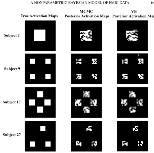
wavelets with 4 vanishing moments; seeDaubechies(1992). As for the selection parameters γiν’s, we chose four patterns of activations as rectangular regions in the 30×30 lattice across the 30 subjects, with subjects 1–7 taking the 1st pattern, subjects 8–15 taking the 2nd pattern, subjects 15–22 taking the 3rd pattern, and subjects 23–30 taking the 4th pattern. The four patterns are shown in the first col-umn of Figure1. Parametersγiν corresponding to the voxels inside the activated regions were assigned the value 1, while those outside were assigned the value 0. This led to 121, 100, 144 and 75 active voxels, out of a total of 900, for patterns 1, 2, 3 and 4, respectively. For active voxels, we set the corresponding regression coefficientsβiν by randomly sampling from a set of 10 different values generated fromN (0, τ0)with τ0=1. We note that our generating mechanism does not im-pose any spatial structure on theβiνparameters. We set the regression coefficients for the inactive voxels to 0. Furthermore, we sampled the innovation variance pa-rametersψiν from a truncated normal distributionN (0, σ02)with support(0,∞) andσ02=1. Finally, we sampled the long memory parametersαiνfrom a uniform distribution in(0,1).
For hyperparameter settings, we setτ =5 for the base distribution of the non-parametric prior (2.5) and fixed the mass parameters toη1=η2=1. We specified a noninformative prior on αiν, that is, a1=b1 =1, and a vague prior on ψiν, that is,a0=3, b0=2. We also set the parameters of the uniform prior onλiν to u1=0, u2=8. Finally, we fixed the MRF prior parameters tod= −2.5, e=0.3. As stated inZhang et al.(2014), the value ofd is chosen to reflect our belief in a sparse model. More specifically,d= −2.5 implies that the prior probability of se-lection is less than 10% when a voxel has no neighbors. The specificatione=0.3 instead was chosen as a value below the phase transition point, which we estimated using the algorithm proposed byPropp and Wilson(1996).
We ran the MCMC with 10,000 iterations and discarded the first 5000 iterations as a burn-in. Convergence was investigated by using the Raftery–Lewis diagnostic [Raftery and Lewis(1992)] as implemented in the R package “coda.” Given the MCMC output, for each subject we obtained a selection of the activated voxels by computing the marginal PPIs and then setting a threshold of 0.01 on the Bayesian
FIG. 1. Simulation study:True activation maps(1st column),posterior estimated maps estimated via MCMC(2nd column)and via variational Bayes(3rd column).Results are shown for one subject for each activation pattern.
False discovery rate for every subject. For the VB algorithm, we used 50 iterations for the inner loop and 600 iterations for the outer loop.
Figure1shows the activation maps estimated via MCMC (second column) and those obtained via VB (third column). Results are given for one subject for each of the true four activation patterns, shown in the first column of the same figure. Estimates appear to be remarkably good, with the VB showing only slightly worse performances and a very few isolated false positives. Figure2shows scatter plots of the posterior estimates ofβandλparameters versus the true values for the same four subjects of Figure 1. Both the MCMC and VB algorithms produce similar estimation results for these parameters. Figure3shows scatter plots for theψand α parameters. Again, all estimates are quite good, with a very small amount of points (voxels) that show posterior estimates which are either higher or lower than
FIG. 2. Simulation study:Scatter plots of posterior estimates of theβandλparameters versus their true values.Results are shown for one subject for each activation pattern.
their true values. These outliers are similar in both the MCMC and VB plots and do not follow any pattern.
Results on the simulated scenario reported above have suggested a very good performance of the VB algorithm in the estimation of the model parameters. A re-markable advantage of inference via VB methods is scalability. In the scenario above, 1000 MCMC iterations took approximately 7 hours using a double core ®Intel ®Xeon processor with 16 GB of memory, 2.2 GHz, while, with VB, 50 iterations of the inner loop with 100 iterations of the outer loop would take ap-proximately 34 minutes. Such computational advantage is particularly important for applications to large data sets, like fMRI data. In order to further assess the per-formance of the VB method, we repeated the simulation 30 times. Table1reports the results on the detection of activated voxels in terms of accuracy, False Negative Rate (FNR), False Positive Rate (FPR), Matthews Correlation Coefficient (MCC) and Area Under the Curve (AUC), averaged over the 30 replicates, for each one of the 30 subjects. Accuracy is defined as the percentage of voxels that are correctly identified, FPR is the proportion of active voxels falsely identified against all the
FIG. 3. Simulation study:Scatter plots of the posterior estimates of theψandαparameters versus their true values.Results are shown for one subject for each activation pattern.
inactive voxels, FNR is the proportion of nonactive voxels falsely identified against all the active voxels, MCC is a correlation coefficient between true and estimated activation status, defined as
MCC=√ TP×TN−FP×FN
(TP+FP)(TP+FN)(TN+FP)(TN+FN),
with TP the number of true positives, TN the number of true negatives, FP the number of false positives, and FN the number of false negatives. Clearly, −1≤MCC≤1, with values closer to 1 indicating better performance. Finally, AUC is the area under the receiver operating characteristic (ROC), a plot of the false positive rate versus the true positive rate, as a measure of the performance of activation detection. Here, we report results on accuracy, FPR, FNR and MCC by setting FDR=0.01 for all subjects. Also, we compute the AUCs by varying the threshold on the posterior probability of inclusionP (γiν=1|data) > c, withc varying on a grid of values from 0 to 1 in steps of 0.01. As expected, the MCMC estimates have a slightly higher accuracy, MCC and AUC values, and a lower FNR than the VB estimates for most of the subjects. Furthermore, all the inactive voxels
TABLE1
Simulation study:Detection of the activated voxels in terms of accuracy,False Negative Rate(FNR), False Positive Rate(FPR),Matthews Correlation Coefficient(MCC)and Area Under the Curve (AUC)for all30subjects,based on the MCMC and Variational Bayes(VB)estimates.Results are
given as averages over30replicated datasets
MCMC Subject 1 2 3 4 5 6 7 8 9 10 Accuracy (%) 94.729 95.211 94.407 96.604 95.063 95.229 95.944 95.867 96.515 96.141 FNR(%) 39.201 35.620 41.598 25.262 36.722 35.482 30.165 37.200 31.367 34.733 FPR (%) 0.000 0.000 0.000 0.000 0.000 0.000 0.000 0.000 0.000 0.000 MCC 0.757 0.781 0.741 0.848 0.774 0.782 0.817 0.774 0.813 0.791 AUC 0.876 0.891 0.867 0.938 0.903 0.900 0.922 0.900 0.909 0.883 Subject 11 12 13 14 15 16 17 18 19 20 Accuracy (%) 96.433 95.341 95.304 95.982 96.652 95.755 95.029 93.692 94.592 95.015 FNR (%) 32.100 41.933 42.267 36.167 30.133 26.528 31.065 39.421 33.796 31.157 FPR (%) 0.000 0.000 0.000 0.000 0.000 0.000 0.000 0.000 0.000 0.000 MCC 0.808 0.743 0.740 0.781 0.820 0.836 0.807 0.751 0.789 0.806 AUC 0.915 0.881 0.865 0.892 0.924 0.922 0.910 0.887 0.904 0.903 Subject 21 22 23 24 25 26 27 28 29 30 Accuracy (%) 94.137 94.604 96.522 97.052 97.455 96.878 96.889 97.033 97.585 96.618 FNR (%) 36.643 33.727 41.733 35.378 30.533 37.467 37.333 35.600 28.978 40.578 FPR (%) 0.000 0.000 0.000 0.000 0.000 0.000 0.000 0.000 0.000 0.000 MCC 0.769 0.789 0.749 0.791 0.822 0.777 0.778 0.790 0.832 0.757 AUC 0.904 0.903 0.880 0.903 0.920 0.865 0.889 0.883 0.927 0.877 VB Subject 1 2 3 4 5 6 7 8 9 10 Accuracy (%) 93.326 93.463 92.282 94.867 93.430 93.585 94.330 94.874 95.352 94.956 FNR (%) 48.705 47.851 56.722 37.135 47.906 46.694 41.047 45.167 40.433 44.500 FPR (%) 0.146 0.120 0.107 0.163 0.150 0.158 0.175 0.121 0.175 0.113 MCC 0.682 0.690 0.621 0.762 0.688 0.696 0.735 0.713 0.741 0.716 AUC 0.853 0.861 0.808 0.866 0.868 0.875 0.875 0.866 0.861 0.861 Subject 11 12 13 14 15 16 17 18 19 20 Accuracy (%) 94.756 94.041 94.622 94.544 95.174 93.578 92.670 91.263 92.196 92.389 FNR (%) 46.000 52.833 47.767 47.967 42.467 39.259 45.023 54.074 47.986 46.852 FPR (%) 0.150 0.100 0.079 0.142 0.121 0.168 0.150 0.101 0.150 0.137 MCC 0.703 0.657 0.697 0.691 0.731 0.744 0.704 0.640 0.682 0.691 AUC 0.831 0.832 0.845 0.852 0.853 0.857 0.846 0.835 0.832 0.854 Subject 21 22 23 24 25 26 27 28 29 30 Accuracy (%) 92.052 92.789 95.863 95.811 96.519 96.322 96.070 96.326 96.748 96.052 FNR (%) 48.958 44.306 48.889 48.489 40.578 42.800 45.867 43.200 37.733 46.0444 FPR (%) 0.137 0.146 0.069 0.162 0.109 0.121 0.117 0.081 0.117 0.121 MCC 0.677 0.710 0.693 0.688 0.748 0.732 0.711 0.732 0.766 0.710 AUC 0.847 0.861 0.817 0.831 0.858 0.881 0.864 0.862 0.875 0.859
TABLE2
Simulation study:Detection of the activated voxels in terms of accuracy(%),for all30subjects, based on the Variational Bayes estimates.Results are for different noise levels and are reported as
percentages for one simulated data
VB Subject 1 2 3 4 5 6 7 8 9 10 ψ=1 94.556 94.556 93.111 96.111 94.667 94.556 95.444 94.778 96.444 96.000 ψ=2 93.222 92.222 91.778 94.111 92.667 92.889 93.889 94.556 95.333 94.444 ψ=4 92.667 91.222 92.111 92.667 91.222 92.333 92.222 93.556 94.778 94.111 ψ=100 90.556 90.667 89.889 92.000 91.000 91.444 91.889 92.333 93.778 92.444 Subject 11 12 13 14 15 16 17 18 19 20 ψ=1 96.111 93.111 95.000 94.889 94.333 94.222 93.556 92.778 93.000 93.222 ψ=2 94.556 93.000 94.333 93.778 94.667 92.444 91.889 89.778 92.444 91.444 ψ=4 93.889 93.000 93.667 93.444 93.222 93.667 90.222 91.333 91.778 90.778 ψ=100 92.556 91.889 93.111 91.667 93.111 90.778 89.111 88.889 89.556 88.222 Subject 21 22 23 24 25 26 27 28 29 30 ψ=1 92.556 93.556 96.222 96.556 97.333 96.889 96.222 96.444 97.556 96.444 ψ=2 90.667 91.889 95.000 95.444 95.778 95.889 95.667 96.000 96.556 95.556 ψ=4 91.333 91.111 95.555 95.111 95.111 95.778 96.000 95.333 96.333 95.222 ψ=100 89.111 88.556 94.333 94.556 94.556 94.778 95.111 94.889 96.000 94.778
are identified correctly by the MCMC method, while a small number of inactive voxels falsely identified as active by the VB method. These results were confirmed when we repeated the simulation study with different noise levels. For example, Table2reports results of the VB algorithm in terms of accuracy for simulated sce-narios with different values of the innovation variance parameterψ. As expected, higher noise levels lead to lower accuracy.
We conclude this section by commenting on the sensitivity of our results to the prior choices. In general, we noticed that modest changes of the values of the vari-ance parameterτ in the base measure of the HDP prior and of the hyperparameters a0, b0, a1, b1, of the prior on the variance parameterψ and the long memory pa-rameterα, did not affect the accuracy of the estimation results. On the other hand, as expected, we noticed some sensitivity to the MRF parameters. In particular, larger values ofdoreled to lower FNRs, at the expense of higher FPRs and lower precisions. As for the concentration parametersη1andη2of the HDP prior, larger values ofη2generated a larger number of components across subjects, while larger values ofη1induced a larger number of within-subject components.
4.2. A comparative study on synthetic data. Here we compare our unified, single-stage estimation method with the two-stage Bayesian hierarchical multi-scale multi-subject method of Sanyal and Ferreira(2012). These authors first fit
FIG. 4. Synthetic data. (First column)True values of regression coefficients; (Second column) Pos-terior estimates of regression coefficients obtained by our method with VB; (Third column)Posterior estimates of regression coefficients obtained by the two-stage method ofSanyal and Ferreira(2012).
a linear model of type (2.1), assuming independent errors and an empirically de-rived subject-specific HRF, obtaining empirical Bayes estimates of the regression coefficients, and then transform the estimated standardized coefficients via DWT to obtain a model in the wavelet space, where they impose spike-and-slab priors on the wavelet coefficients. Their method is implemented in the R package “BHMS-MAfMRI.”
Following a simulation strategy similar to the one adopted byQuirós, Diez and Gamerman(2010), we simulated synthetic fMRI data as the sum of two compo-nents,Ysyn=y+w, whereyis simulated from our model and where the intercept parameterwis a selected slice, at a fixed time point, from real fMRI data. We con-sidered 27 subjects, with three different activation patterns, as shown in the first column in Figure4. The true values of βiν in the active brain regions were ran-domly sampled from a set of 10 different values, generated from a Uniform(0,80). The innovation variance parameters ψiν were sampled from a truncated normal
FIG. 5. Synthetic Data:ROC curves based on normalized estimates of the regression coefficients, for both our method and the two-stage method ofSanyal and Ferreira(2012).
distribution with mean 0 and variance 80. The data dimension for each subject was 256 scans of 64×64 voxels.
We report here the results of our model with variational Bayes inference. As we have demonstrated above, this inferential procedure achieves robust estimation results at reduced computational costs, therefore allowing scalability of our meth-ods. Here we setτ =50 for the base distribution of the nonparametric prior (2.5) and fixed the mass parameters to η1=η2=1. As done in the simulation stud-ies above, we specified a noninformative prior on αiν, that is, a1 =b1 =1, a vague prior on ψiν, that is, a0 =3, b0 =2, and fixed the MRF prior param-eters to d = −2.5, e=0.3. Finally, we set the hyperparameters of the uniform prior onλiν tou1=0, u2=5. We ran the VB algorithm, combined with impor-tance sampling, by setting the number of outer loop (imporimpor-tance sampling) itera-tions ton=100 and the number of inner loop (variational inference) iterations to m=10.
To keep the comparison fair, we applied both our method and the multiscale multi-subject method ofSanyal and Ferreira(2012) using wavelet transforms with Daubechies wavelets with 4 vanishing moments. Both methods took approxi-mately 1.5 hours to run. Figure4shows the true and posterior mean maps of the regression coefficients for three of the subjects, for both our method and the mul-tiscale method of Sanyal and Ferreira (2012). The plots demonstrate that, while both methods can detect relevant activations in the truly activated areas, the two-stage method also identifies spurious activations in truly inactive areas, especially for subjects 7 and 18. Furthermore, Figure5shows receiver operating character-istic (ROC) curves calculated by plotting sensitivity (true positive rate) versus 1-specificity (false positive rate), averaged over the 30 subjects, for different values of a threshold. In this plot, a voxel is declared active if the regression coefficient estimate corresponding to that voxel is larger than the threshold. To obtain each point on the ROC curve, we varied the threshold within the standard Gaussian
quantiles corresponding to cumulative probabilities between 0 and 1 in steps of 0.01. Figure 5 clearly shows the improved performance of our method. We also ran the VB algorithm with a higher number of inner and outer loop iterations, ob-taining an ROC curve very similar to the one we report in Figure 5 (result not shown).
In their paper,Sanyal and Ferreira(2012) obtain also group-level posterior maps by averaging the posterior coefficient maps across all subjects. An additional fea-ture of our modeling approach is that the use of the nonparametric HDP prior construction (2.5) can be exploited to obtain a clustering of the subjects for possi-ble discovery of differential activations. Even though the HDP construction does not allow a direct estimation of cluster memberships, a dissimilarity matrix can be constructed by computing the squared Euclidean distances between each pair of subjects as
dij=
(Biˆ − ˆBj)T(Biˆ − ˆBj),
withBiˆ denoting the posterior estimate ofBi=(βi1, . . . , βiV)T, i=1, . . . , N. The dissimilarity matrix can then be transformed into a tree via hierarchical cluster-ing. Figure 6 shows the cluster dendrogram obtained using the linkage method with Ward’s minimum variance and the group maps for the three largest clus-ters, obtained by averaging the posterior maps of theβ coefficients in each clus-ter. In this figure, the distance calculation and the group maps were obtained using only the nonzero βiν’s, that is, those corresponding to γiνˆ =1. Alterna-tively, one could consider distancesdij’s weighted by the posterior probabilities P (γiν=1|data). The clustering recovers the simulated structure of the data per-fectly, and the group maps show an accurate estimation of the different activation patterns.
4.3. A case study for fMRI data. We apply our model to real fMRI data col-lected as part of an experiment conducted at the Department of Behavioral Science at the University of Texas MD Anderson Cancer Center [Versace et al.(2013)].
The study aimed at assessing brain responses to natural visual scenes. During the experiment, brain responses from 27 female participants to emotional and neu-tral stimuli were measured using a picture-viewing procedure. Sixty pictures from five categories were presented, with twelve pictures each showing neutral people (NEU), erotic couples (ERO), romantic couples (ROM), mutilations (MUT) and sad scenes (SAD). The picture presentation consisted of two blocks, each lasting for approximately 12 minutes. Each picture was shown for 5 s, followed by an intertrial interval ranging from 15 s to 20 s. In order to minimize the effect of the picture presentation order, each participant was randomly assigned to one of the five picture presentation sequences. During picture presentation, fMRI data were recorded using a 3.0 T Discovery MR750, 32-channel MRI system. The BOLD signal was measured using a T2∗-weighted, echo-planar, parallel imaging protocol
FIG. 6. Synthetic data: (Top)Cluster dendrogram obtained with hierarchical clustering under the linkage method. (Bottom)Posterior group-level maps ofβfor the3largest clusters.
with a 2.5 s repetition time, 25 ms echo time and 90◦ flip angle. Data were col-lected as 58 contiguous 3-mm coronal slices, 64×64 imaging matrix and 2.5 mm ×2.5 mm in-plane resolution, resulting in full brain coverage with a spatial reso-lution of 2.5×2.5×3 mm. The first two volumes in each picture-viewing block were discarded to allow magnetization to reach a steady state. Thus, a collection of 286 volumes were used in our estimation procedure.
The processed data consisted of smoothed, spatially standardized, motion and slice-timing corrected images. In order to make the signal level consistent at corre-sponding voxels across subjects, we transformed the data by percent signal change normalization, that is, we set yt∗=yt/y¯ ×100, with yt the signal in a voxel at time pointtandy¯ the mean of the voxel signal time courses. We then applied our Bayesian nonparametric model with VB to the normalized data y∗. We defined the stimulus function as a vector with elements set to 1, indicating when the par-ticipant was looking at the images, and to 0 when the parpar-ticipant was presented blank pictures. We convolved the stimulus vector with a Poisson hemodynamic function with voxel-dependent and subject-specific parameterλiνto obtain the co-variateXiν.
FIG. 7. Case study data:Results for the occipital slice(y= −60mm)in three subjects. (First col-umn)Posterior activation maps obtained with our multi-subject method; (Second Column)Activation maps obtained with SPM8and the method ofFriston and Penny(2003). (Third Column)Activation maps obtained with the single-subject estimation method ofZhang et al.(2014).
When fitting the model to the data we set τ =50 for the base distribution of the nonparametric prior (2.5) and fixed the mass parameters toη1=η2 =1. As done in the simulation studies, we specified a noninformative prior on αiν, that is,a1=b1=1, a vague prior onψiν, that is,a0=3, b0=2, and fixed the MRF prior parameters tod= −2.5, e=0.3. Finally, we set the hyperparameters of the uniform prior onλiν tou1=0, u2=5. We ran the VB algorithm, combined with importance sampling, by setting the number of outer loop (importance sampling) iterations to 600 and the number of inner loop (variational inference) iterations to 50.
We present the results of our analysis on a coronal slice covering the occipi-tal cortex, with locationy= −60 mm in the Talairach space, as it is well known that visual stimuli increase activation of the visual areas. Figure 7(first column) shows the posterior activation maps for 3 of the subjects. Activations are clearly detected. The multiscale method ofSanyal and Ferreira (2012) could not be ap-plied here because it assumes the same stimulus function across all subjects, while
in our experimental setting the picture presentation sequence varies among sub-jects. For comparison, we therefore looked into the estimation results from single-subject methods. Figure7(second column) shows the posterior probability activa-tion maps for the 3 subjects produced by the software SPM8 following the method of Friston and Penny (2003), who considered a Bayesian spatiotemporal model with autoregressive errors and a spatial prior onβ. With this approach, the poste-rior probability that a particular effect exceeds a thresholdκ is calculated as
(4.2) p=1− κ−wTMβ|y wTCβ |yw ,
with Mβ|y and Cβ|y the posterior mean and covariance of the parameter β. In particular, we obtained the maps in Figure7(second column) by applying an F-contrast with F-contrast weight vectorw= [1,0]T to the estimation of the regression coefficients, and using a threshold of 0.999. In the third column of Figure7 we shows activation maps obtained by applying the single-subject Bayesian model of
Zhang et al.(2014) which, like our method, assumes long-memory errors and a spike-and-slab prior on theβ coefficients. This comparison clearly shows that a multi-subject modeling strategy leads to a more accurate detection of the activated areas, with respect to approaches that carry out estimation on single subjects. Fur-thermore, in order to better appreciate the accuracy of the detection, in Figure8we report results on a coronal slice chosen in the frontal areas, where passive viewing of visual stimuli, when averaged across valences, are not expected to lead to in-creased brain activation. Indeed, many spurious activations can be observed in the maps estimated via the single-subject approaches.
The current paradigm in neuroimaging suggests that locations are either “active” or “inactive” at the population level [Rosenblatt, Vink and Benjamini(2014)]. In-deed, for the fMRI experimental study we have considered here, with all healthy subjects, one should not expect spatial activation patterns to be widely distinct across subjects. In our modeling setting, an all-subject posterior map can be read-ily obtained by averaging the posterior maps of theβ coefficients across all sub-jects. This map is reported in Figure9for the occipital slice, and correctly shows activations in the visual areas. Additionally, as pointed out in the analysis of syn-thetic data of the previous section, our modeling approach allows us to obtain a clustering of the subjects based on different characteristics of their activations. For example, the cluster-level maps for the two largest clusters, obtained using the link-age method with Ward’s minimum variance and then averaging the posterior maps of theβ coefficients in each cluster, are also shown in Figure9. Both maps show activations in the visual areas, as expected, and, additionally, highlight groups of subjects with possible differences in intensity, as subjects in cluster 1 show clear lower effects than those in cluster 2.
FIG. 8. Case study data:Results for the frontal slice(y= +38mm)in three subjects. (First column) Posterior activation maps obtained with our method; (Second column)Activation maps obtained with SPM8and the method ofFriston and Penny(2003). (Third column)Activation maps obtained with the single-subject estimation method ofZhang et al.(2014).
5. Conclusions. In this paper we have proposed a unified, probabilistically coherent framework for the analysis of task-related brain activity in multi-subject fMRI experiments. Our modeling approach has shown improved estimation perfor-mance on simulated data, with respect to two-stage approaches which separate the inference on the individual fMRI time courses from the inference at the population level. The proposed model builds upon the large literature on spatiotemporal linear regression models by specifically accounting for the between-subjects heterogene-ity in neuronal activheterogene-ity. The model formulation, in particular, extends the single-subject approach ofZhang et al.(2014), which also employs long-memory errors and variable selection priors, to incorporate a spatially informed multi-subject non-parametric spike-and-slab variable selection prior on the regression coefficients. Furthermore, posterior inference is carried out via a variational Bayes algorithm that allows scalability.
We have shown, on simulated data, that inference via variational Bayes achieves satisfactory results at more reduced computational costs than using a Markov chain
FIG. 9. Case study data: (Top)Cluster dendrogram obtained with hierarchical clustering under the linkage method for the occipital slice(y= −60mm). (Bottom)Posterior group-level maps ofβ
for the2largest clusters and for all subjects.
Monte Carlo algorithm. We have also demonstrated that our probabilistically co-herent modeling approach for multiple subjects achieves improved estimation per-formance with respect to two-stage approaches. Finally, in an application to case study data, our method has successfully detected activations in the occipital areas during presentation of visual stimuli, whereas no activations have been detected in the frontal areas. We have also shown that a multi-subject modeling strategy leads to a more accurate detection of the activated areas than single-subject models, such as that ofZhang et al.(2014). This is an important stepping stone in the develop-ment of reliable detection methods that can be applied to full brain datasets and complex experimental designs.
A single fMRI experiment can yield hundreds of thousands of high frequency time series for each subject, arising from spatially distinct locations. The strategy we have adopted in this paper has been to study the brain activations of all voxels in targeted regions of the brain, for example, regions known to respond to pleas-ant stimuli, like the prefrontal cortex. Alternatively, some existing approaches for fMRI data analysis achieve dimension reduction by considering a partition of the whole brain into regions of interest (ROIs) that can be defined in terms of structural
or functional features, for example, based on anatomically weighted probabilistic maps [Tzourio-Mazoyer et al. (2002)]. For example, the two-stage modeling ap-proach ofBowman et al.(2008) for multiple subjects comprises a first stage where a voxel-wise GLM is fitted for each subject, assuming serially correlated errors and a prespecified HRF, and a second stage that considers an anatomical par-cellation of the brain and applies a Bayesian hierarchical model to region-based contrast responses to detect task-related activated regions. Our unified modeling framework is general and can be applied, in principle, to whole-brain 3D data. However, given the large dimensionality of 3D data, some type of dimension re-duction might be needed, even when using the VB algorithm for inference. For example, one strategy can be to partition the brain into regions of interest, sum-marizing the voxel time courses into area-based time series and fitting the model to the area-based data, according to the assumption that the pattern of activity in brain areas is more important than the activity of single neurons or voxels [Joset, Gazzola and Keysers(2009)]. Given the parcellation of the brain, a spatial MRF prior can then be defined based on the Euclidean distance between the centroids of the ROIs.
In this paper we have considered spatially informed multi-subject nonparamet-ric variable selection priors of type (2.5) that employ the hierarchical Dirichlet process ofTeh et al.(2006) to induce clustering of the regression coefficientsβiν’s within as well as among subjects. Alternative choices we are currently investigat-ing include the nested Dirichlet Process ofRodríguez, Dunson and Gelfand(2008), which allows to cluster entire distributions across subjects, and multivariate con-ditionally auto-regressive (CAR) models [Banerjee, Carlin and Gelfand (2015)], since theβij ν’s are expected to change smoothly over space. Furthermore, to possi-bly aid the interpretation of the clusters, Dependent Bayesian nonparametric priors [Barrientos, Jara and Quintana(2012)], that let the cluster assignment probabilities to depend on available covariates, can be used.
In the applications, we have so far investigated single-threaded matlab imple-mentations of both the MCMC and variational Bayes algorithms. Further compu-tational benefit may result by exploring parallel computing, in particular, by taking advantage of the Matlab built-in support for GPU computation, which will allow us to substantially speed up expensive operations within single iterations [see, e.g.,
Yan, Xu and Qi(2009) for a GPU implementation of VB algorithms]. SUPPLEMENTARY MATERIAL
Supplement to “A spatiotemporal nonparametric Bayesian model of multi-subject fMRI data” (DOI: 10.1214/16-AOAS926SUPP; .pdf). The supplemen-tary material [Zhang et al. (2016)] contains a detailed description of the MCMC steps and of the VB inner and outer loops.
REFERENCES
BANERJEE, S., CARLIN, B. P. and GELFAND, A. E. (2015).Hierarchical Modeling and Analysis for Spatial Data, 2nd ed.Monographs on Statistics and Applied Probability135. CRC Press, Boca Raton, FL.MR3362184
BARRIENTOS, A. F., JARA, A. and QUINTANA, F. A. (2012). On the support of MacEachern’s dependent Dirichlet processes and extensions.Bayesian Anal.7277–309.MR2934952
BISHOP, C. M. (2006). Pattern Recognition and Machine Learning. Springer, New York.
MR2247587
BLEI, D. M. and JORDAN, M. I. (2006). Variational inference for Dirichlet process mixtures. Bayesian Anal.1121–143 (electronic).MR2227367
BOWMAN, F., CAFFO, B., BASSETT, S. and KILTS, C. (2008). A Bayesian hierarchical framework for spatial modeling of fMRI data.NeuroImage39146–156.
BUXTON, R. and FRANK, L. (1997). A model for the coupling between cerebral blood flow and oxygen metabolism during neural stimulation.J.Cereb.Blood Flow Metab.1764–72.
CARBONETTO, P. and STEPHENS, M. (2012). Scalable variational inference for Bayesian variable selection in regression, and its accuracy in genetic association studies.Bayesian Anal.773–107.
MR2896713
DAUBECHIES, I. (1992).Ten Lectures on Wavelets.CBMS-NSF Regional Conference Series in Ap-plied Mathematics61. SIAM, Philadelphia, PA.MR1162107
EFRON, B. (2008). Microarrays, empirical Bayes and the two-groups model.Statist.Sci.231–22.
MR2431866
FADILI, M. J. and BULLMORE, E. T. (2002). Wavelet-generalised least squares: A new BLU esti-mator of linear regression models with 1/f errors.NeuroImage15217–232.
FERGUSON, T. S. (1973). A Bayesian analysis of some nonparametric problems.Ann.Statist.1 209–230.MR0350949
FLANDIN, G. and PENNY, W. D. (2007). Bayesian fMRI data analysis with sparse spatial basis function priors.NeuroImage341108–1125.
FRISTON, K. J. (1994). Functional and effective connectivity in neuroimaging: A synthesis.Hum. Brain Mapp.256–78.
FRISTON, K. J. (2011). Functional and effective connectivity: A review.Brain Connectivity113–36. FRISTON, K. J., JEZZARD, P. and TURNER, R. (1994). Analysis of functional MRI time-series.
Hum.Brain Mapp.1153–171.
FRISTON, K. J. and PENNY, W. (2003). Posterior probability maps and SPMs.NeuroImage191240– 1249.
FRISTON, K. J., HOLMES, A. P., POLINE, J. B., GRASBY, P. J., WILLIAMS, S. C. R., FRACK
-OWIAK, R. S. J. and TURNER, R. (1995). Analysis of fMRI time-series revisited.NeuroImage2 45–53.
FRISTON, K. J., PENNY, W., PHILLIPS, C., KIEBEL, S., HINTON, G. and ASHBURNER, J. (2002). Classical and Bayesian inference in neuroimaging: Theory.NeuroImage16465–483.
HARRISON, L. M. and GREEN, G. G. R. (2010). A Bayesian spatiotemporal model for very large data sets.NeuroImage501126–1141.
HARTVIG, N. V. and JENSEN, J. L. (2000). Spatial mixture modeling of fMRI data.Hum.Brain Mapp.11233–248.
HOLMES, A. P. and FRISTON, K. J. (1998). Generalisability, random effects & population inference. Neuroimage7S754.
ISHWARAN, H. and JAMES, L. F. (2001). Gibbs sampling methods for stick-breaking priors.J.Amer. Statist.Assoc.96161–173.MR1952729
JBABDI, S., WOOLRICH, M. W. and BEHRENS, T. E. J. (2009). Multiple-subjects connectivity-based parcellation using hierarchical Dirichlet process mixture models.NeuroImage44373–384. JEONG, J., VANNUCCI, M. and KO, K. (2013). A wavelet-based Bayesian approach to regres-sion models with long memory errors and its application to fMRI data.Biometrics69184–196.
MR3058065
JOHNSON, T. D., LIU, Z., BARTSCH, A. J. and NICHOLS, T. E. (2013). A Bayesian non-parametric Potts model with application to pre-surgical FMRI data.Stat.Methods Med.Res.22364–381.
MR3190664
JOSET, A. E., GAZZOLA, V. and KEYSERS, C. (2009). An introduction to anatomical ROI-based fMRI classification analysis.Brain Res.1282114–125.
KALUS, S., SÄMANN, P. G. and FAHRMEIR, L. (2014). Classification of brain activation via spatial Bayesian variable selection in fMRI regression.Adv.Data Anal.Classif.863–83.MR3168680
KIM, S., SMYTH, P. and STERN, H. (2006). A nonparametric Bayesian approach to detecting spatial activation patterns in fMRI data. InMedical Image Computing and Computer-Assisted Intervention–MICCAI2006 217–224.
LEE, K.-J., JONES, G. L., CAFFO, B. S. and BASSETT, S. S. (2014). Spatial Bayesian variable selection models on functional magnetic resonance imaging time-series data.Bayesian Anal.9 699–731.MR3256061
LI, F., ZHANG, T., WANG, Q., GONZALEZ, M. Z., MARESH, E. L. and COAN, J. A. (2015). Spatial Bayesian variable selection and grouping for high-dimensional scalar-on-image regression.Ann. Appl.Stat.9687–713.MR3371331
LINDQUIST, M. A. (2008). The statistical analysis of fMRI data. Statist. Sci. 23 439–464.
MR2530545
MEYER, F. G. (2003). Wavelet-based estimation of a semiparametric generalized linear model of fMRI time-series.IEEE Trans.Med.Imag.22315–322.
MÜLLER, P., PARMIGIANI, G. and RICE, K. (2007). FDR and Bayesian multiple comparisons rules. InBayesian Statistics8 (J. M. Bernardo, M. J. Bayarri, J. O. Berger, A. P. Dawid, D. Heckerman, A. F. M. Smith and M. West, eds.).Oxford Sci.Publ. 349–370. Oxford Univ. Press, Oxford.
MR2433200
NEWTON, M. A., NOUEIRY, A., SARKAR, D. and AHLQUIST, P. (2004). Detecting differential gene expression with a semiparametric hierarchical mixture method.Biostatistics5155–176. PENNY, W., KIEBEL, S. and FRISTON, K. J. (2003). Variational Bayesian inference for fmri time
series.NeuroImage19727–741.
PENNY, W. D., TRUJILLO-BARRETO, N. and FRISTON, K. J. (2005). Bayesian fMRI time series analysis with spatial priors.NeuroImage24350–362.
PROPP, J. G. and WILSON, D. B. (1996). Exact sampling with coupled Markov chains and applica-tions to statistical mechanics. InProceedings of the Seventh International Conference on Random Structures and Algorithms(Atlanta,GA, 1995)9223–252. Random Structures Algorithms, 1-2.
MR1611693
QUIRÓS, A., DIEZ, R. M. and GAMERMAN, D. (2010). Bayesian spatiotemporal model of fMRI data.NeuroImage49442–456.
RAFTERY, A. E. and LEWIS, S. M. (1992). One long run with diagnostics: Implementation strategies for Markov chain Monte Carlo.Statist.Sci.7493–497.
RODRÍGUEZ, A., DUNSON, D. B. and GELFAND, A. E. (2008). The nested Dirichlet process.
J.Amer.Statist.Assoc.1031131–1144.MR2528831
ROSENBLATT, J. D., VINK, M. and BENJAMINI, Y. (2014). Revisiting multi-subject random effects in fMRI: Advocating prevalence estimation.NeuroImage84113–121.
RUE, H., MARTINO, S. and CHOPIN, N. (2009). Approximate Bayesian inference for latent Gaus-sian models by using integrated nested Laplace approximations. J. R. Stat. Soc. Ser. B Stat. Methodol.71319–392.MR2649602
SANYAL, N. and FERREIRA, M. A. (2012). Bayesian hierarchical multi-subject multiscale analysis of functional MRI data.NeuroImage631519–1531.
SAVITSKY, T. and VANNUCCI, M. (2010). Spiked Dirichlet process priors for Gaussian process models.J.Probab.Stat. Art. ID 201489, 14.MR2745498
SAVITSKY, T., VANNUCCI, M. and SHA, N. (2011). Variable selection for nonparametric Gaussian process priors: Models and computational strategies.Statist.Sci.26130–149.MR2849913
SETHURAMAN, J. (1994). A constructive definition of Dirichlet priors.Statist.Sinica4639–650.
MR1309433
SMITH, M. and FAHRMEIR, L. (2007). Spatial Bayesian variable selection with application to func-tional magnetic resonance imaging.J.Amer.Statist.As