Targeted maximum likelihood estimation for a binary treatment: A tutorial.

(2018) Targeted maximum likelihood estimation for a binary treat-ment: A tutorial. Statistics in medicine. ISSN 0277-6715 DOI: https://doi.org/10.1002/sim.7628

Downloaded from: http://researchonline.lshtm.ac.uk/4647544/

DOI:10.1002/sim.7628

Usage Guidelines

Please refer to usage guidelines at http://researchonline.lshtm.ac.uk/policies.html or alterna-tively [email protected].

T U T O R I A L I N B I O S T A T I S T I C S

Targeted maximum likelihood estimation for a binary

treatment: A tutorial

Miguel Angel Luque

‐

Fernandez

| Michael Schomaker

| Bernard Rachet

|

Mireille E. Schnitzer

1_{Cancer Survival Group, Department of}

Non‐Communicable Disease

Epidemiology, Faculty of Epidemiology and Population Health, London School of Hygiene and Tropical Medicine, London, UK

2_{Department of Epidemiology, Harvard T.}

H. Chan School of Public Health, Boston, MA, USA

3_{Biomedical Research Institute of}

Granada, Non‐Communicable and Cancer Epidemiology Group (ibs.Granada), Andalusian School of Public Health, Granada, Spain

4_{School of Public Health and Family}

Medicine, Center for Infectious Disease Epidemiology and Research, The University of Cape Town, Cape Town, South Africa

5_{Faculté de pharmacie, Université de}

Montréal, Montréal, Canada Correspondence

Miguel Angel Luque‐Fernandez, Cancer Survival Group, Department of Non_‐ Communicable Disease Epidemiology, Faculty of Epidemiology and Population Health, London School of Hygiene and Tropical Medicine, UK Keppel Street, London WC1E 7HT, UK.

Email: miguel_‐[email protected] Funding information

Canadian Institutes of Health Research; Carlos III Institute of Health, Grant/ Award Number: CP17/00206; Cancer Research UK, Grant/Award Number: C7923/A18525

When estimating the average effect of a binary treatment (or exposure) on an outcome, methods that incorporate propensity scores, the G‐formula, or targeted maximum likelihood estimation (TMLE) are preferred over naïve regression approaches, which are biased under misspecification of a parametric outcome model. In contrast propensity score methods require the correct spec-ification of an exposure model. Double‐robust methods only require correct specification of either the outcome or the exposure model. Targeted maximum likelihood estimation is a semiparametric double‐robust method that improves the chances of correct model specification by allowing for flexible estimation using (nonparametric) machine‐learning methods. It therefore requires weaker assumptions than its competitors. We provide a step‐by‐step guided implemen-tation of TMLE and illustrate it in a realistic scenario based on cancer epidemi-ology where assumptions about correct model specification and positivity (ie, when a study participant had 0 probability of receiving the treatment) are nearly violated. This article provides a concise and reproducible educational introduction to TMLE for a binary outcome and exposure. The reader should gain sufficient understanding of TMLE from this introductory tutorial to be able to apply the method in practice. Extensive R‐code is provided in easy‐to‐ read boxes throughout the article for replicability. Stata users will find a testing implementation of TMLE and additional material in the Appendix S1 and at the following GitHub repository: https://github.com/migariane/SIM‐TMLE‐ tutorial

K E Y W O R D S

causal inference, ensemble Learning, machine learning, observational studies, targeted maximum likelihood estimation

-This is an open access article under the terms of the Creative Commons Attribution License, which permits use, distribution and reproduction in any medium, provided the original work is properly cited.

© 2018 The Authors.Statistics in Medicinepublished by John Wiley & Sons Ltd. DOI: 10.1002/sim.7628

1

|

I N T R O D U C T I O N

During the last 30 years, modern epidemiology has been able to identify significant limitations of classic epidemiologic methods when the focus is to explain the effect of a risk factor on a disease or outcome.1,2In observational studies, treat-ment groups are typically not directly comparable; thus, a careful statistical adjusttreat-ment for confounders is necessary to obtain unbiased exposure (or treatment) effect estimates. Failure to account for confounding variables, namely, those preexposure variables associated with both the exposure and the outcome, can result in a biased estimate.3Causal infer-ence based on the Neyman‐Rubin potential outcome framework4allows researchers to carefully adjust for confounders under structural causal assumptions. The framework was first introduced in the social sciences by Rubin5and later in epidemiology and biostatistics by Greenland and Robins.6

Causal effects are often formulated in potential outcomes, as formalised by Rubin.4Let A denote a binary exposure, Wa preexposure vector of potential confounders, and Y a binary outcome. Each individual has a pair of potential out-comes: the outcome they would have received had they been exposed (A = 1), denoted Y(1), and the outcome had they been unexposed, Y(0). However, it is only possible to observe a single realisation of the outcome for an individual. We observe Y(1) only for those in the exposure group and Y(0) only for those in the unexposed group.4,5Common causal estimands of interest are the average treatment effect (ATE), defined as E[Y(1)−Y(0)], and the marginal odds ratio (MOR), defined as E[Y(1)] × {1−E[Y(0)]}/{E(1−E[Y(1)]) × E[Y(0)]}.

To identify the ATE, classical epidemiologic methods, such as standard regression models where the treatment is included as a covariate in the analysis, require the assumption that the effect measure of the treatment of interest is con-stant across the levels of confounders included in the model.7However, in observational studies, this is often not the case. In 1986, a seminal paper6demonstrated that under untestable causal assumptions (conditional exchangeability, positivity, consistency, and noninterference), a consistent estimate of the ATE can be obtained by using the G‐formula6 (a generalisation of standardisation with respect to the confounder distribution):

ATE¼∑ W ∑y P Yð ¼yjA¼1;W¼wÞ−∑ y P Yð ¼yjA¼0;W¼wÞ " # P Wð ¼wÞ

G‐computation,8based on the estimation of the components in the G‐formula, allows for a treatment effect that may vary across the levels of the confounders. This approach relies on parametric modelling assumptions and bootstrap for the estimation of the standard error. Therefore, G‐computation is sensitive to model misspecification9,10and requires time‐consuming estimation of confidence intervals (CIs).

Alternatively, the propensity score11 can also be used for estimation of the ATE. Propensity score methods, intro-duced by Rosenbaum and Rubin,12estimate the treatment mechanism. In our setting, where treatment is assigned at a single time point, the propensity score is defined as the probability of being treated given the observed confounders W, denoted P(A = 1|W). The propensity score is used to statistically balance exposure groups in their preexposure covar-iates to estimate the ATE. This may be done via matching, weighting, or stratification.13,14 When weighting by the inverse of the propensity score, extreme values of the propensity score can lead to large weights, resulting in unstable ATE estimates with high variance (in particular, ATE estimates can fall outside the constraints of the statistical model). Furthermore, when analysing observational data with a large number of variables and potentially complex relationships among them, model misspecification is of particular concern in this case as well.10Hence, correct model specification is crucial to obtain unbiased estimates of the true ATE.10,14,15Overall, the above‐mentioned methods can be classified as those focused on modelling the outcome‐generating function of treatment and confounders (ie, G‐computation) and those focused on modelling the treatment‐generating function of confounders (ie, propensity‐score methods).

Double‐robust methods were developed to minimise the impact of model misspecification.10,16,17 Double‐robust methods require estimation of both the outcome and treatment mechanisms. For the estimation of the ATE in our exam-ple, the outcome mechanism is the conditional expectation of the outcome given the exposure and the covariates, denoted E(Y|A,W), and the treatment mechanism corresponds to the propensity score, which is the conditional proba-bility of being treated given the observed confoundersW, denoted P(A = 1|W). Double‐robust means that the estimator is consistent as long as either the outcome model or the treatment model is estimated consistently. Some double‐robust estimators are also locally semiparametric efficient, meaning that the estimator has minimal large sample variance among estimators that make the same model assumptions, under the correct specification of the required models.10,16,18 Current simulation‐based evidence shows that the use of double‐robust and locally efficient methods such as the aug-mented inverse probability of treatment weighted (AIPTW) and the targeted maximum likelihood estimation (TMLE)

method estimators often outperform the G‐computation and propensity score methods, in both point and interval esti-mation.10,16,19However, AIPTW is less robust to data sparsity and near violations of the practical positivity assumption than TMLE (ie, when certain subgroups in a sample rarely receive some treatment of interest).10,16,19

Targeted maximum likelihood estimation, a general template for the construction of efficient and double‐robust sub-stitution estimators, was first introduced by Van der Laan and Rubin in 200620but is based on existing methods.18,21This approach first requires a specification of the statistical model, corresponding with what restrictions are being placed on the data‐generating distribution. For the ATE, the TMLE procedure requires initial estimates of E(Y|A,W) and P(A = 1| W), and then includes a substitution“targeting”step that optimises the bias‐variance tradeoff for the targeted parameter (e.g., the ATE). Furthermore, one can readily use ensemble and machine‐learning algorithms to estimate E(Y|A,W) and P(A = 1|W), thus avoiding model misspecification.10

Targeted maximum likelihood estimation respects the limits of the possible range of the targeted parameter, reduces bias through the use of ensemble and machine‐learning algorithms, and, finally, makes statistical inference quick and easy based on the efficient influence curve (IC).19,20,22,23Evidence shows that TMLE can provide consistent ATE esti-mates in challenging settings and has a smaller asymptotic variance compared with other (nonefficient) double‐robust estimators.10,19,24Mathematically, TMLE and AIPTW are both efficient and have the same asymptotic properties. In par-ticular, they both have the minimum asymptotic variance in their class of semiparametric estimators. However, TMLE is a substitution estimator and behaves differently in finite sample settings producing estimates in the range of values of the parameter space while AIPTW does not.10,19,24

The statistical properties of TMLE make it a suitable tool for applied researchers aiming to estimate causal effects. The TMLE procedure is available in standard statistical software such as thetmlepackage19implemented in the statis-tical software R (R Foundation for Statisstatis-tical Computing, Vienna, Austria). Users familiar with other software can also easily use TMLE, for example, by using our test version for a TMLE implementation in Stata or simply by importing their data to R (see Appendix S1).

We provide a step‐by‐step guided implementation of TMLE by using a simulated example inspired by population‐ based cancer research.25We aim to demystify TMLE and show applied medical statisticians how they can easily adopt the method for their applications. In contrast to many other papers, we demonstrate the implementation of TMLE in a realistic setting with many challenges such as near‐positivity violations (ie, manifested by large inverse probability of treatment weights) and misspecification of both the treatment and outcome models. We also show the implementa-tion of AIPTW and the benefit of incorporating advanced machine‐learning algorithms to reduce bias. We provide commented R code embedded in boxes as well as Stata code in the Appendix S1, making our results fully reproducible.

2

|

M O T I V A T I O N A L E X A M P L E , C A U S A L M O D E L , A N D D A T A

G E N E R A T I O N

The motivating example was developed to estimate the 1‐year mortality risk difference and odds ratio of death (Y) for cancer patients treated with monotherapy (only radiotherapy; A = 1) versus dual therapy (treatment with radiotherapy and chemotherapy; A = 0) while controlling for possible confounders (W).25,26To be able to consistently estimate the ATE, the data must satisfy the following assumptions: (i) Cancer treatment is independent of the potential mortality out-comes after conditioning onW(ie, (Y(0), Y(1))⊥A|W). This assumption is often referred to as“conditional exchangeabil-ity”and one cannot test it using the observed data. It implies that (within the strata ofW) the mortality risk under the potential treatment A = 1, ie, P(Y(1) = 1|A = 1,W) equals the one under treatment A = 0, ie, P(Y(1) = 1|A = 0,W). In other words: the risk of death for those treated would have been the same as for those untreated if untreated subjects had received, contrary to the fact, the treatment. This is equivalent to assuming that all confounders have been measured. (ii) We also assume that within strata ofW, every patient had a nonzero probability of receiving either of the 2 treatment conditions, ie, 0 < P(A = 1|W) < 1 (positivity). (iii) We assume consistency, which states that we observe the potential outcome corresponding with the observed treatment, ie, for any individual, Y = AY(1) + (1−A)Y(0). Also, (iv) in defin-ing an individual's counterfactual outcome as only a function of their own treatment, we assume noninterference, mean-ing that the counterfactual outcome of one subject was not influenced by the treatment of any other. Under the causal assumptions explained above, the ATE may be consistently estimated in the nonparametric model (that does not impose assumptions on either E(Y|A,W) or P(A = 1|W)). Thus, if we believe these assumptions to hold and the sample size to be sufficient, we may interpret our estimate of the ATE approximately as the marginal risk difference of 1‐year mortality for cancer patients treated with monotherapy versus dual therapy.

2.1

|

Data generation process

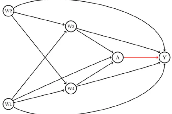
To demonstrate the implementation of TMLE, we generated data, denoted as the set of i.i.d variables O = (W= (W1,W2, W3,W4), A, Y), based on the directed acyclic graph1illustrated in Figure 1.

Briefly, sex (W1) and age category (W2) were generated as Bernoulli variables with probabilities 0.5 and 0.65, respec-tively. Cancer stage (W3) and comorbidities (W4) were generated as ordinal variables with 4 and 5 levels, respectively. For both variables, we used a random uniform distribution with minimum 0 and maximum 4 and 5, respectively, and rounded the generated numbers off to the closest integer. The treatment variable (A) and the potential outcomes (Y(1) and Y(0)) were generated as binary indicators using log‐linear models. In the treatment and outcome models, we included an interaction term between age (W2) and comorbidities (W4) based on plausible biological mechanisms such as an increased risk of comorbidities among older adults.26 Another, more complex data generating process can be found in Appendix S1.

The data‐generating model for the treatment was selected to create the potential for near‐practical positivity viola-tions. In particular, given the possible covariate values and the coefficients, the minimum possible true probability of receiving treatment was 0.002. Finally, for simplicity, we did not include effect modification (ie, interaction between A andW) though both TMLE and AIPTW can easily handle this setting as well.

First, we generated a sample of 5 million patients to estimate the true ATE and MOR. Afterwards, we generated a sample of 10 000 patients used to illustrate the implementation of the algorithm and run simulations. In Box 1, we intro-duce the specifications for the data generation and the true values for the ATE and the MOR. The true ATE implies that the risk of death among cancer patients treated with monotherapy is approximately 19.3% higher than for those treated with dual therapy. The true MOR implies that there is a 2.5 times higher odds of death among cancer patients treated with monotherapy versus dual therapy. Note that for educational purposes, we present the code and results for a single dataset simulated by our data‐generating mechanism. However, at the end of the illustration, we also present the results of 1000 Monte Carlo simulations with a sample size of 1000 patients aiming (i) to estimate the bias of the estimators under near‐positivity violations and mild misspecification of the treatment and outcome models and (ii) to demonstrate TMLE's double‐robustness property by misspecifying the model for the outcome.

FIGURE 1 Direct acyclic graph. Legend: Conditional exchangeability of the treatment effect or exposure (A) on cancer mortality (Y) is obtained through conditioning on a set of available covariates (Y(1),Y(0)⊥A|W). The average treatment effect for the structural

framework is estimated as the average risk difference between the expected effect of the treatment conditional onWamong those treated (E(Y|A = 1;W)) and the expected effect of the treatment conditional onWamong those untreated (E(Y|A = 0;W)). Y: mortality binary indicator (1 death, 0 alive), A: binary treatment for cancer with monotherapy versus dual therapy (1 Mono; 0 Dual);W:W1: sex;W2: age at

diagnosis;W3: cancer stage, TNM classification;W4: comorbidities [Colour figure can be viewed at wileyonlinelibrary.com]

Box 1 Data generation

# Function to generate data generateData <- function(n) {

w1 <-rbinom(n, size = 1, prob = 0.5) w2 <-rbinom(n, size = 1, prob = 0.65)

In Box 1,plogis(x)represents the inverse logit function: exp xð Þ 1þexp xð Þ.

3

|

T M L E A L G O R I T H M : G U I D E D I M P L E M E N T A T I O N

In this section, we introduce the step‐by‐step implementation of the TMLE algorithm in a set of 10 boxes with docu-mented R code for educational reproducibility.

3.1

|

TMLE implementation

Targeted maximum likelihood estimation can either be used by means of thetmlefunction from the R‐packagetmleor by computing the algorithm in 6 steps manually. We first show the latter option for educational purposes; a sound under-standing of TMLE will enable the reader to make the right decisions for their analysis.

First step: Prediction of the outcome model bar Q0(A,W) = E(Y|A,W)

The superscript 0 in Q0ðA;WÞindicates that it is the initial estimate of E(Y|A,W), which is the conditional mean of the outcome (Y) given treatment A and baseline covariatesW. To obtain Q0(A,W), we can use a standard logistic regres-sion model:

logit½P Yð ¼1jA;WÞ ¼β₀þβ₁AþβT₂W wherelogit(x) represents the function log x

1‐x

andβis the vector of the estimates for the coefficients of the model parameters. As before, A represents the treatment andWis the transpose of the vector of covariatesW= (W1,…,W4) presented in the DAG (Figure 1).

w3 <-round(runif(n, min = 0, max = 4), digits = 0) w4 <-round(runif(n, min = 0, max = 5), digits = 0)

A <-rbinom(n, size = 1, prob =plogis(-5 + 0.05*w2 + 0.25*w3 + 0.6*w4 + 0.4*w2*w4)) # counterfactual

Y.1 <-rbinom(n, size = 1, prob =plogis(-1 + 1 - 0.1*w1 + 0.35*w2 + 0.25*w3 + 0.20*w4 + 0.15*w2*w4)) Y.0 <-rbinom(n, size = 1, prob =plogis(-1 + 0 - 0.1*w1 + 0.35*w2 + 0.25*w3 + 0.20*w4 + 0.15*w2*w4)) # observed outcome

Y <- Y.1*A + Y.0*(1 - A) # return data.frame

data.frame(w1, w2, w3, w4, A, Y, Y.1, Y.0) }

# True ATE and OR set.seed(7777)

ObsData <-generateData(n = 5000000) True_EY.1 <-mean(ObsData$Y.1) True_EY.0 <-mean(ObsData$Y.0)

True_ATE <- True_EY.1 - True_EY.0; True_ATE

True_MOR <- (True_EY.1*(1 - True_EY.0))/((1 - True_EY.1)*True_EY.0); True_MOR #True_ATE: 19.3%

#True_MOR: 2.5 # Data for simulation set.seed(7722)

Therefore, we can estimate the initial probabilities as the prediction of this logistic outcome regression model for A = 0 and A = 1, respectively (Box 2):

Q0ð0;WÞ ¼expitbβ₀þbβ₁0þbβT₂Wand Q0ð1;WÞ ¼expit bβ0þbβ11þbβT2W

; whereexpit(x)represents the inverse logit function expð Þx

1þexpð Þx .

Note that for educational purposes, we misspecified both the propensity score and outcome models by not accounting for the interaction between age (W2) and comorbidities (W4). This allows us to later show the added value of incorporat-ing machine‐learning algorithms for prediction.

As computed at the bottom of Box 2, the G‐computation (untargeted) estimate is the mean of Q0ð1;WÞ−Q0ð0;WÞ, taken over all subjects. In this case, this is a very good estimate of the ATE and the MOR because the outcome model is nearly correctly specified.

Second step: Prediction of the propensity scorebgðA;WÞ

In this step, we estimate P(A = 1|W), the probability of the treatment with monotherapy versus dual therapy (A) given the set of covariates (W), namely, the propensity score. Using a logistic regression model, we set

logit P A½ ð ¼1jWÞ ¼α0þαT1W: We then estimate the probabilitiesbg 1ð ;WÞusing

b

g 1ð ;WÞ ¼expit bα0þbαT1W

wherebα0andbα1are the estimates of the coefficients in the logistic regression.

Box 2 Prediction ofQ0ðA;WÞ

#First estimation of E(Y|A,W), namely Q0ðA;WÞ

m <-glm(Y ~ A + w1 + w2 + w3 + w4, family = binomial, data = ObsData) #Misspecified model #Prediction for A, A = 1 and, A = 0

QAW =predict(m, type ="response")

Q1W =predict(m, newdata = data.frame(A = 1, ObsData[,c("w1","w2","w3","w4")]), type ="response") Q0W =predict(m, newdata = data.frame(A = 0, ObsData[,c("w1","w2","w3","w4")]), type ="response") #Estimated mortality risk difference (G‐computation)

mean(Q1W - Q0W)

#Initial ATE estimate:20.4% #Estimated MOR (G-computation)

mean(Q1W)*(1 -mean(Q0W)) / ((1 -mean(Q1W))*mean(Q0W)) #Initial MOR estimate:2.7

Box 3 Prediction of the propensity scorebg 1ð ;WÞ

psm <-glm(A ~ w1 + w2 + w3 + w4, family = binomial, data = ObsData) #Misspecified model gW =predict(psm, type ="response") #propensity score values

Note that as in the previous step, here in Box 3, we intentionally did not account for the interaction between age (W2) and comorbidities (W4) in the treatment model. Also, the summary of the estimated propensity score (gW) indicates near violations of the practical positivity assumption given the very small numbers for the lower tail of the distribution, an interesting setting under which to compare TMLE with AIPTW.

The next 2 steps aim to improve the prediction model Q0ðA;WÞfrom step 1 by incorporating information from the propensity score. This can be viewed as updating Q0ðA;WÞalong a path to incorporate additional information from the propensity score function with the goal of reducing the residual confounding in the first estimate of Q0ðA;WÞ.

Third step: The clever covariate and estimation ofε

This step aims to compute the clever covariates H(1,W) and H(0,W), and a vector fluctuation parameter calledε. The clever covariates in Equation 1 are calculated for each individual in the data, based on their previously estimated probabilities of exposure status, P(A = 1|W) and P(A = 0|W). Note that the functional forms of the clever covariates are very similar to inverse probability of treatment weights:

H 1ð ;WÞ ¼ A

bg 1ð ;WÞ; H 0ð ;WÞ ¼ 1‐A

bg 0ð ;WÞ: (1) The fluctuation parameter bε¼ðbε0;bε1Þis estimated through a maximum likelihood procedure; we set a model with the observed outcome (Y) as dependent variable and the logit of the initial prediction of Q0ðA;WÞas an offset (fixed quantity) in an intercept‐free logistic regression with the clever covariates, H(1,W) and H(0,W) as independent variables (Box 4): E Yð ¼1jA;WÞð Þ ¼ε 1 1þ exp −log Q 0 A;W ð Þ 1−Q0ðA;WÞ −ε0H 0ð ;WÞ−ε1H 1ð ;WÞ 0 @ 1 A : (2)

When there is little variability in Y−Q0ðA;WÞ(ie, the outcome minus the offset), the fluctuation parameter will be esti-mated as close to 0. In the absence of residual confounding, the propensity score does not provide additional information to improve the initial estimate of Q0ðA;WÞ because Q0ðA;WÞwas correctly specified. Given a misspecified Q0ðA;WÞ; the fluctuation parameter may also be estimated as approximately 0 when bg 1ð ;WÞhas no supplementary information relevant to Y. However, TMLE is consistent as long as either the model or the treatment model is estimated consistently. The clever covariates are called“clever”because their form guarantees that the estimating equation corresponding to the efficient IC is solved, which in turn yields desirable (asymptotic) inferential properties, including double‐robustness and local efficiency. A complete explanation of how the clever covariates are chosen is given in van der Laan and Rose,10 Chapter 5.

In Box 4, we show how to compute the clever covariates and how to estimateε. Note thatqlogis(x)represents the logit function in R.

Box 4 Computation of the clever covariates, H(1,W) and H(0,W), and estimation ofbε

#Clever covariate and fluctuating/substitution parameters H1W = (ObsData$A / gW)

H0W = (1 - ObsData$A) / (1 - gW) #Propensity score distribution summary(gW)

Min. 1st Qu. Median Mean 3rd Qu. Max. 0.002 0.03 0.086 0.155 0.240 0.718

Alternatively, one could add the clever covariates not as covariates, but as weights in this same update step. This is another valid targeted maximum likelihood estimator, based on a refined loss function (and parametric sub model), and can improve stability.10

Fourth step: Update of Q0ðA;WÞto Q1ðA;WÞ

The updated estimate of E(Y|A,W) is denoted Q1ðA;WÞ. This update is performed by plugging inbε¼ðbε0;bε1Þinto the following equations (Box 5):

Q1ð0;WÞ ¼expit logit Q0ð0;WÞ

þbε0=bg 0ð ;WÞ

h i

and Q1ð1;WÞ ¼expit logit Q0ð1;WÞ

þbε1=bg 1ð ;WÞ

h i

: (3) In this way, the update is done separately under the treatment and under the control by evaluating both of these expressions for all subjects.

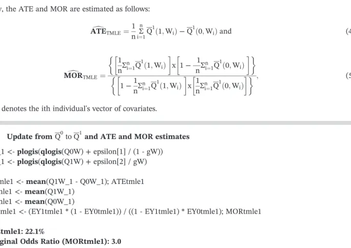
Fifth step: Targeted estimate of the ATE and the MOR Finally, the ATE and MOR are estimated as follows:

d ATETMLE¼ 1 nΣ n i¼1Q 1 1;Wi ð Þ−Q1ð0;WiÞand (4) d MORTMLE¼ 1 nΣ n i¼1Q 1 1;Wi ð Þ x 1− 1 nΣ n i¼1Q 1 0;Wi ð Þ 1−1 nΣ n i¼1Q 1 1;Wi ð Þ x 1 nΣ n i¼1Q 1 0;Wi ð Þ ; (5)

whereWidenotes the ith individual's vector of covariates.

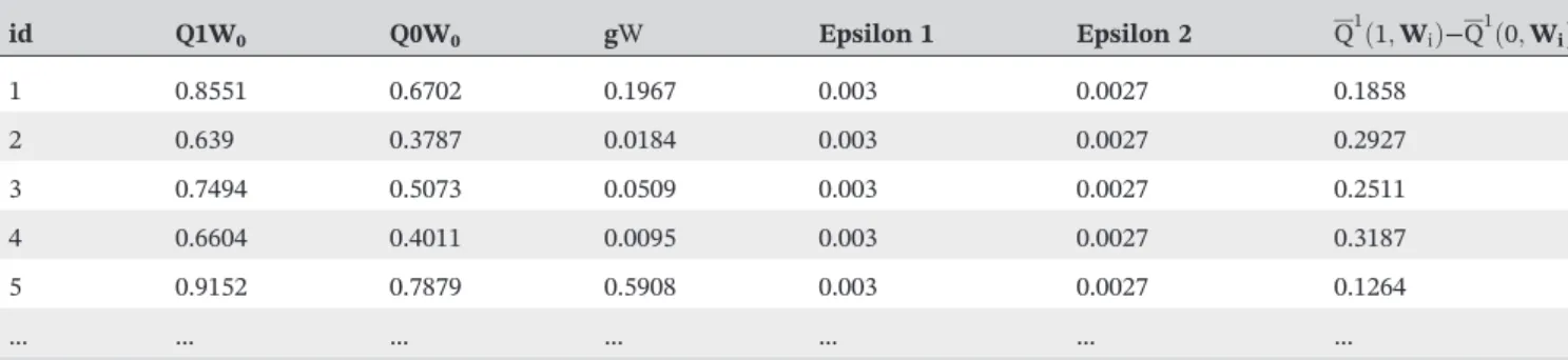
Table 1 shows the first 5 rows of the final dataset where the predicted value of Q1ð1;WÞ−Q1ð0;WÞfor the first patient (id = 1) can be estimated by using Equation 3 as the inverse logit transformation of the initial estimates Q0ð1;WÞand Q0ð0;WÞplus the estimated fluctuation parameter epsilonð Þbε times the clever covariates as follows:

Box 5 Update fromQ0to Q1and ATE and MOR estimates

Q0W_1 <-plogis(qlogis(Q0W) + epsilon[1] / (1 - gW)) Q1W_1 <-plogis(qlogis(Q1W) + epsilon[2] / gW) ATEtmle1 <-mean(Q1W_1 - Q0W_1); ATEtmle1 EY1tmle1 <-mean(Q1W_1)

EY0tmle1 <-mean(Q0W_1)

MORtmle1 <- (EY1tmle1 * (1 - EY0tmle1)) / ((1 - EY1tmle1) * EY0tmle1); MORtmle1 #ATEtmle1: 22.1%

#Marginal Odds Ratio (MORtmle1): 3.0

epsilon <- coef(glm(ObsData$Y ~ -1 + H0W + H1W + offset(qlogis(QAW)), family = binomial)); epsilon #epsilon:0.003, 0.003

Q1ð1;WiÞ−Q 1 0;Wi ð Þ ¼plogis qlogis Q0ð1;WiÞ þbε1=bg 1ð ;WiÞ −plogis qlogis Q0ð0;WiÞ þbε0=bg 0ð ;WiÞ

plogis(qlogis(Q1W_0) + epsilon[2] / gW)−plogis(qlogis(Q0W_0) + epsilon[1] / (1‐gW))=0.1858 Sixth step: Statistical inference and 95% CI

Targeted maximum likelihood estimation constructs estimators based on the efficient IC,19,20which can be used to obtain standard errors. Based on semiparametric and empirical processes theory, the IC of a consistent and asymptoti-cally linear estimator is derived in the gradient of the pathwise derivative of the target parameter such that27,28

d ATE‐ATE¼1 nΣ n i¼1ICi‐Op 1 ffiffiffi n p : (6)

By the weak law of the large numbers, the Opterm in equation (6) converges to 0 at a rate of 1

ffiffiffi n

p as the sample size (n) goes to infinity.10The IC is a function of the data and the data‐generating components that one can derive for a given model and target parameter that has mean 0 and finite variance. The central limit theorem applies so that in large sam-ples, the variance of the estimator is thus the variance of the IC divided by n. While many influence functions and cor-responding estimators exist for a given target parameter, there always exists an“efficient”IC that achieves the lower bound on asymptotic variance for the given set of modelling assumptions. Targeted maximum likelihood estimation and AIPTW are both constructed by using the efficient IC, making these estimators asymptotically efficient for the sta-tistical model when all necessary models are correctly specified. For the ATE, the efficient IC is

EICATE¼ A P Að ¼1jWÞ− 1−A P Að ¼0jWÞ Y−E Yð jA;WÞ ½ þE Yð jA¼1;WÞ−E Yð jA¼0;WÞ−ATE;

which can be evaluated as

d EICATE¼ A bg 1ð ;WÞ− 1−A bg 0ð ;WÞ Y−Q1ðA;WÞ h i þQ1ð1;WÞ−Q1ð0;WÞ−ATEdTMLE (7)

for every subject. Using the resulting vector, the estimation of the standard error forATEdTMLEis done as follows:

b

σATE;TMLE ¼

ffiffiffiffiffiffiffiffiffiffiffiffiffiffiffiffiffiffiffiffiffiffiffiffiffiffiffiffiffi d

Var EICdATE

n v u u t ; (8)

wheredVar EICdATE

represents the“sample variance”of the estimated IC. TABLE 1 Final dataset for the update of Q0ðA;WÞto Q1ðA;WÞ

id Q1W0 Q0W0 gW Epsilon 1 Epsilon 2 Q 1 1;Wi ð Þ−Q1ð0;WiÞ 1 0.8551 0.6702 0.1967 0.003 0.0027 0.1858 2 0.639 0.3787 0.0184 0.003 0.0027 0.2927 3 0.7494 0.5073 0.0509 0.003 0.0027 0.2511 4 0.6604 0.4011 0.0095 0.003 0.0027 0.3187 5 0.9152 0.7879 0.5908 0.003 0.0027 0.1264 … … … …

Based on the functional Delta method,29the efficient IC for the MOR is EICMOR¼ 1−E Y 0½ ð Þ 1−E Y 1½ ð Þ ð Þ2 x E Y 0½ ð Þ× D1− E Y 1½ ð Þ 1−E Y 1½ ð Þ ð Þx E Y 0ð ½ ð ÞÞ2× D0; (9) where D1 and D0 are the efficient IC for E[Y(1)] and E[Y(0)], respectively:

D1¼ A P Að ¼1jWÞ Y−E Yð jA¼1;WÞ ½ þE Yð jA¼1;WÞ−E Y 1½ ð Þ; (10) D0¼ 1−A P Að ¼0jWÞ Y−E Yð jA¼0;WÞ ½ þE Yð jA¼0;WÞ−E Y 0½ ð Þ: (11)

In Box 6, it is shown how to evaluate the efficient IC for the ATE and the MOR based on Equations 5 to 11.

3.2

|

Comparative performance of TMLE: TMLE vs naïve logistic regression approach and

AIPTW

In Box 7, we show the estimation and results of the naïve logistic regression approach, which assumes a correctly spec-ified parametric outcome model (violated in the example below) and a constant effect of the treatment (A) on 1‐year mortality (not violated in the example below). In addition, because of the noncollapsibility of the odds ratio, even a cor-rectly specified logistic regression model generally does not produce estimates of the MOR.

Box 6 Estimation of the SE and 95% CI for theATEdTMLEandMORd TMLE

#ATE efficient influence curve (EIC)

D1 <- ObsData$A/gW*(ObsData$Y - Q1W_1) + Q1W_1 - EY1tmle1

D0 <- (1 - ObsData$A)/(1 - gW)*(ObsData$Y - Q0W_1) + Q0W_1 - EY0tmle1 EIC <- D1 - D0

#ATE variance n <-nrow(ObsData) varHat.IC <-var(EIC)/n #ATE 95%CI

ATEtmle1_CI <- c(ATEtmle1 - 1.96*sqrt(varHat.IC), ATEtmle1 + 1.96*sqrt(varHat.IC)); ATEtmle1; ATEtmle1_CI

#ATEtmle1_CI(95%CI): 22.1% (15.1, 29.0) #MOR EIC

EIC <- (1 - EY0tmle1) / EY0tmle1 / (1 - EY1tmle1)^2 * D1 - EY1tmle1 / (1 - EY1tmle1) / EY0tmle1^2 * D0 varHat.IC <-var(EIC)/n

#MOR 95%CI

MORtmle1_CI <- c(MORtmle1 - 1.96*sqrt(varHat.IC), MORtmle1 + 1.96*sqrt(varHat.IC)); MORtmle1; MORtmle1_CI

AIPTW, which directly uses the efficient IC, can also be used to estimate the ATE and the MOR. The ATE and MOR using AIPTW are computed as follows:

d EY1AIPTW ¼1 n Σ n i¼1 I Aið ¼1Þ b g 1ð ;WiÞ Yi−Q0ð1;WiÞ þQ0ð1;WiÞ : d EY0AIPTW ¼ 1 n Σ n i¼1 I Að i¼0Þ b g 0ð ;WiÞ Yi−Q 0 0;Wi ð Þ þQ0ð0;WiÞ : d

ATEAIPTW¼EY1AIPTWd −EY0dAIPTW: (12)

d

MORAIPTW ¼

d

EY1AIPTW 1−EY0dAIPTW

1−EY1AIPTWd d EY0AIPTW; (13)

whereWidenotes the ith individual's vector of covariates.

In Box 8, we provide code for the estimation of the ATE and the MOR (with variances and CIs) using AIPTW.

Box 7 Estimation of the conditional odds ratio using the naïve logistic regression approach

Naive <-glm(data =ObsData, Y ~ A + w1 + w2 + w3 + w4, family = binomial) summary(Naive)

exp(Naive$coef[2]) exp(confint(Naive))

#Naïve OR (95%CI): 2.9 (2.5, 3.4)

Box 8 Estimation of the ATE and MOR using AIPTW

EY1aiptw <-mean((ObsData$A) * (ObsData$Y - Q1W) / gW + Q1W)

EY0aiptw <-mean((1 - ObsData$A) * (ObsData$Y - Q0W) / (1 - gW) + Q0W) AIPTW_ATE <- EY1aiptw - EY0aiptw; AIPTW_ATE

AIPTW_MOR <- (EY1aiptw * (1 - EY0aiptw)) / ((1 - EY1aiptw) * EY0aiptw); AIPTW_MOR #Calculation of the efficient IC

D1 <- (ObsData$A) * (ObsData$Y - Q1W) / gW + Q1W - EY1aiptw

D0 <- (1 - ObsData$A) * (ObsData$Y - Q0W) / (1 - gW) + Q0W - EY0aiptw varHat_AIPTW <-var(D1 - D0) / n

ATEaiptw_CI <- c(AIPTW_ATE - 1.96*sqrt(varHat_AIPTW), AIPTW_ATE + 1.96*sqrt(varHat_AIPTW)); AIPTW_ATE; ATEaiptw_CI

#ATEaiptw_CI(95%CI): 24.0% (16.4, 31.6)

ICmor_aiptw <- (1 - EY0aiptw) / EY0aiptw / (1 - EY1aiptw)^2 * D1 - EY1aiptw / (1 - EY1aiptw) / EY0aiptw^2 * D0

varHat_AIPTW2 <-var(ICmor_aiptw) / n

MORaiptw_CI <- c(AIPTW_MOR - 1.96*sqrt(varHat_AIPTW2), AIPTW_MOR + 1.96*sqrt(varHat_AIPTW2)); AIPTW_MOR; MORaiptw_CI

3.3

|

TMLE improved performance calling the Super

‐

Learner

Note that in the one‐sample simulation illustrated so far, we have intentionally misspecified both models (treatment and outcome) to allow for evaluation of the benefit of calling theSuperLearner (SL) R package (Boxes 9 and 10). The SL, which is a type ofensemble learner, adaptively combines different machine‐learning algorithms to (separately) estimate Q0ðA;WÞandbg Að ;WÞ. The aim of including this approach in the TMLE algorithm is to avoid bias arising from model misspecification.10SL thus replaces the simple logistic models in steps 1 and 2 above. One generally selects a set of pre-diction algorithms for use in the SL, which may include parametric regression models, nonlinear regression models, shrinkage estimators, and regression trees. Instead of choosing the algorithm with the smallest expected prediction error (estimated by cross validation), the SL selects a weighted combination of different algorithms. Specifically, it selects the weighted combination of predictions that minimises the cross‐validated mean square error (Supplementary Figure S1).30 It can be shown that this weighted combination will perform asymptotically at least as well as the best algorithm (in the cross‐validated error), but typically even better.10,19,23,30Box 9 describes the implementation of TMLE using the R‐ pack-age“tmle”while calling the SL. The basic implementation of TMLE in the R‐packagetmleuses by default 3 algorithms: “SL.glm”(logistic regression using A andWas covariates),“SL.step”(stepwise model selection ofWin a generalized linear model using Akaike's information criterion to determine subsets of the full model), and “SL.glm.interaction”(a generalised linear model that includes all 2‐way interactions of the terms included in the full model).23To list all imple-mented algorithms, one can simply type“listWrappers()”in R. In Box 10, we illustrate the reduction of bias by calling, in addition to default algorithms implemented intmle, more advanced machine‐learning algorithms such as generalised additive models, random forests, and recursive partitioning. For a more advanced theoretical background regarding machine‐learning algorithms, see Hastie et al.31

Box 9 TMLE using default implementation with the default SL library

library(tmle)

library(SuperLearner)

TMLE2 <-tmle(Y = ObsData$Y, A = ObsData$A, W = ObsData[,c("w1","w2","w3","w4")], family ="binomial") ATEtmle2 <- TMLE2$estimates$ATE$psi;ATEtmle2 TMLE2$estimates$ATE$CI MORtmle2 <- TMLE2$estimates$OR$psi;MORtmle2 TMLE2$estimates$OR$CI #ATEtmle2 (95%CI): 20.8% (17.5, 24.1) #MORtmle2 (95%CI): 2.8 (2.3, 3.4)

Box 10 TMLE with a user‐selected SL library

library(tmle)

library(SuperLearner)

SL.library <- c("SL.glm","SL.step","SL.step.interaction","SL.glm.interaction","SL.gam", "SL.randomForest","SL.rpart")

TMLE3 <-tmle(Y = ObsData$Y,A = ObsData$A,W = ObsData [,c("w1","w2","w3","w4")], family ="binomial", Q.SL.library = SL.library,g.SL.library = SL.library)

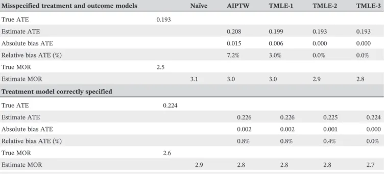
Table 2 summarises the results of 1000 Monte Carlo simulations each with a sample size of 1000 patients based on the data generation process introduced in Box 1. We present the ATE and MOR estimates for 3 different estimators (naïve regression, AIPTW, and TMLE) and 3 different versions of TMLE (TMLE‐1‐2‐3, Table 2) corresponding to the usage of either logistic regressions or SL, implemented either with the default or user‐supplied library given in Box 10, for the estimation of the outcome expectation and the propensity score. Furthermore, our data generation often pro-duced near‐practical positivity violations (ie, certain subgroups in the samples rarely or never received treatment) as described above. We checked the violation visually (Figure 2) and numerically, based on the empirical summary of the propensity score distribution (mean = 0.189, min = 0.002 and max = 0.765). In the logistic regressions, the models for the treatment and the outcome were misspecified by omitting the interactions between age and comorbidities. Finally, to demonstrate the TMLE double‐robustness property, we ran a second set of simulations when correctly spec-ifying the propensity score using the true logistic regression model (with the outcome model either incorrectly specified with a main term logistic regression or adaptively estimated with SL). Complete details of the models'functional forms for the data generation and the full settings for the simulation are provided in the Appendix S1 and at the following GitHub repository: https://github.com/migariane/SIM‐TMLE‐tutorial, making our results fully reproducible.

TABLE 2 ATE and COR Monte Carlo simulations for mild misspecified models and near‐positivity violation, n = 1000

Misspecified treatment and outcome models Naïve AIPTW TMLE‐1 TMLE‐2 TMLE‐3

True ATE 0.193

Estimate ATE 0.208 0.199 0.193 0.193

Absolute bias ATE 0.015 0.006 0.000 0.000

Relative bias ATE (%) 7.2% 3.0% 0.0% 0.0%

True MOR 2.5

Estimate MOR 3.1 3.0 3.0 2.9 2.8

Treatment model correctly specified

True ATE 0.224

Estimate ATE 0.226 0.226 0.225 0.224

Absolute bias ATE 0.002 0.002 0.001 0.000

Relative bias ATE (%) 0.8% 0.8% 0.4% 0.0%

True MOR 2.6

Estimate MOR 2.9 2.8 2.8 2.8 2.7

d

ATE:Estimated average treatment effect from the 1000 simulation repetitions.

d

MOR:Estimated marginal odds ratio from the 1000 simulation repetitions. Naïve:Logistic regression.

AIPTW:Augmented inverse‐probability treatment weights estimation under dual misspecification (model for the treatment and the outcome). TMLE‐1:Dual misspecification. Algorithm computed by hand and naïve prediction (using from logistic regression models) without Super‐Learner (SL). TMLE‐2:Dual misspecification. Algorithm estimated using R‐packagetmleand default SL library (SL.glm, SL.step, and SL.glm.interaction).

TMLE‐3:Dual misspecification. Algorithm computed using R‐packagetmle,user‐supplied SL library (SL.gam, SL.randomForest, and SL.rpart).

Treatment model correctly specified refers to the usage of the correct logistic regression model for the propensity score. For TMLE‐2 and TMLE‐3, SL is used to estimate the outcome model as in the first scenario.

TMLE3$estimates$ATE$CI

MORtmle3 <- TMLE3$estimates$OR$psi;MORtmle3 TMLE3$estimates$OR$CI

#ATEtmle3 (95%CI): 20.7% (17.5, 24.0) #MORtmle3 (95%CI): 2.7 (2.2, 3.3)

In this example, the true ATE is 19.3% and the MOR of monotherapy versus dual therapy was 2.5. The results of the different estimators are presented in Table 2. The naïve approach overestimated the MOR by 24%, whereas the AIPTW and TMLE‐1 overestimated it by 20%, likely because of model misspecification. However, TMLE‐3, which used a more diverse SL library, reduced the bias for the MOR to 12%. Regarding the simulation results for the risk differences, the AIPTW estimator overestimated the ATE by 7%, whereas TMLE‐1 overestimated it by just 3%. However, TMLE‐2 and TMLE‐3 reduced the bias for the ATE to 0%. Therefore, the introduction of machine‐learning algorithms and ensemble learning as discussed above reduced the bias of TMLE‐2 and TMLE‐3. Finally, under misspecification of the outcome model, but correct specification of the propensity score model, the TMLE‐3 was unbiased for the ATE and the MOR.

4

|

D I S C U S S I O N

The quantity, quality, and variety of available data for observational epidemiology continue to grow extensively, making the estimation of causal effects more accessible and popular among applied statisticians and epidemiologists. Targeted maximum likelihood estimation implemented with ensemble and machine‐learning algorithms has advantages over other methods, but surprisingly there is limited guidance for the application of the technique for the estimation of the ATE and MOR when dealing with binary outcomes.32 By using a reproducible example, we have demonstrated that the implementation of the TMLE algorithm is not a black box. Using a guided step‐by‐step approach, we have provided the basic elements needed to understand how TMLE works. Furthermore, we have demonstrated the positive benefit, in bias reduction and performance, of adding more advanced machine‐learning algorithms to the fitting process of TMLE. Our educational example adds to other already available tutorials,32-36but with a different motivation based on popula-tion‐based cancer epidemiology, a clear orientation towards applied statisticians, and fully explained and available code to replicate step‐by‐step the implementation of TMLE in both Stata and R statistical software. However, our simulation scenarios were relatively simple. We simulated categorical and binary variables and did not produce interaction between the treatment and the vector of confounders, which might not be a realistic setting. Allowing for effect modification (interaction between A andW) is an interesting case, because this is a specific setting where the naïve regression adjust-ment does not work. Despite that, the main interest of the illustration was to introduce the step‐by‐step implementation of the TMLE algorithm and demonstrate the added value of adding machine and ensemble learning algorithms for pre-diction. Readers will find an additional example with treatment effect modification in Appendix S1 where we used the R‐packagesimcausal.

FIGURE 2 Probability density function of the propensity score by treatment status for one randomly selected sample from 1000 Monte Carlo simulations [Colour figure can be viewed at wileyonlinelibrary.com]

The implementation of TMLE for the estimation of the ATE with a continuous outcome follows identical steps to those listed above. However, note that for this case, (i) we first transform the outcome via Y−a/(b−a), where a and b are plausible values for lower and upper limits of Y; (ii) proceed with the steps from the tutorial; and (iii) rescale the estimate of the ATE and the variance at the end. Readers can find additional depth including the mathematical der-ivation of TMLE in Chapter 7 of the Targeted Learning book.10

Adding more adaptive SuperLearner algorithms requires a significant amount of computer memory and computa-tional time. Hence, with large sample sizes, such as those in population‐based cancer research, TMLE will benefit from additional computing resources such as a cluster environment. For instance, for a computer with 1 core and 16 GB of memory, the R‐package tmle took 5.4 minutes to estimate the ATE for 10 000 patients using more advanced machine‐learning algorithms including generalised additive models, random forests, and boosting. Furthermore, some machine‐learning algorithms will not work properly depending on the nature of the observed data (eg, for small sample sizes or nonbinary outcomes). Moreover, some theoretical background knowledge of machine learning is required to decide for the most adaptive SL algorithms.

Using TMLE in practical settings is similar to the strategy used for analysts when applying other double‐robust methods such as AIPTW (eg, summarising the inverse probability of treatment weights, checking the distribution of the weights by levels of the treatment, and considering if appropriate the truncation of the weights). Also, we suggest considering the extent to which the data allow for very complicated machine‐learning algorithms, a question closely related with the dimensionality of the data (ie, for small datasets and continuous outcomes, some machine learning might not perform well). Finally, we suggest that readers aiming to develop TMLE approaches follow the causal roadmap introduced above and described by Van der Laan and coauthors.10Similarly, readers can find additional depth including the mathematical derivation of TMLE in Chapter 5 of the Targeted Learning book.10

It is important to mention that TMLE is a general template for the construction of efficient substitution estimators for a given estimation problem defined by a statistical model and a targeted parameter. Targeted maximum likelihood estimation is a very active research area, and many advances have been and are currently being made. Clearly, these advances have not been covered here in our introductory tutorial, but a reader might be interested in such topics as the TMLE for rare outcomes,37the Collaborative TMLE for the cross‐validated conditional risk of a candidate estimator,38-40 and the TMLE for longitudinal settings where time‐dependent confounding is an issue.34,41-43

In summary, we have provided an accessible presentation with documented code for implementing TMLE to esti-mate the ATE and MOR for a binary outcome in observational studies. Given TMLE's appealing statistical properties, we consider it a suitable method to be added to the analytical toolbox for estimation of causal effects in large popula-tion‐based observational studies.

A U T H O R S'C O N T R I B U T I O N S

MALF developed the concept and design of the study. MALF carried out the simulations and analysed the data and wrote the manuscript. All authors interpreted the data, drafted and revised the manuscript, code, and results critically. All authors read and approved the final version of the manuscript. MALF is the guarantor of the paper.

A C K N O W L E D G E M E N T S

This work was supported by Cancer Research UK grant number C7923/A18525. M.A.L.F. is supported by a Miguel Servet I Investigator Award (grant CP17/00206) from the Carlos III Institute of Health, and M.E.S. is supported by a Canadian Institutes of Health Research New Investigator Award. The findings and conclusions in this report are those of the authors and do not necessarily represent the views of the funding agencies. The corresponding author had full access to all the data in the study and had final responsibility for the decision to submit for publication.

O R C I D

Miguel Angel Luque‐Fernandez http://orcid.org/0000-0001-6683-5164 Michael Schomaker http://orcid.org/0000-0002-8475-0591

R E F E R E N C E S

1. Pearl J.Causality : models, reasoning, and inference. 2nd ed. Cambridge: Cambridge University Press; 2009.

2. Robins JM, Hernan MA, Brumback B. structural models and causal inference in epidemiology.Epidemiology. 2000;550‐560. 3. Rothman K.Modern Epidemiology. 4th ed. Philadelphia: Lippincott Williams & Wilkins; 2016.

4. Rubin DB. inference using potential outcomes.J Am Stat Assoc. 2011;100(469):322‐331.

5. Rubin DB. Estimating causal effects of treatments in randomized and nonrandomized studies.J Educ Psychol. 1974;66(5):688. 6. Greenland S, Robins JM. Identifiability, exchangeability, and epidemiological confounding.Int J Epidemiol. 1986;15(3):413‐419. 7. Keil AP, Edwards JK, Richardson DB, Naimi AI, Cole SR. The parametric g‐formula for time‐to‐event data: intuition and a worked

exam-ple.Epidemiology. 2014;25(6):889‐897.

8. Snowden JM, Rose S, Mortimer KM. Implementation of G‐computation on a simulated data set: demonstration of a causal inference tech-nique.Am J Epidemiol. 2011;173(7):731‐738.

9. Manski CF.Identification for Prediction and Decision. Cambridge, Mass. London: Harvard University Press; 2007.

10. van der Laan M, Rose S.Targeted Learning: Causal Inference for Observational and Experimental Data. New York: Springer Series in Sta-tistics; 2011.

11. Austin PC. An introduction to propensity score methods for reducing the effects of confounding in observational studies.Multivariate Behav Res. 2011;46(3):399‐424.

12. Rosenbaum PR, Rubin DB. The central role of the propensity score in observational studies for causal effects.Biometrika. 1983;70(1):41‐55. 13. Guo S, Fraser MW.Propensity Score Analysis: Statistical Methods and Applications. Second ed. SAGE: Los Angeles; 2015.

14. Lunceford JK, Davidian M. Stratification and weighting via the propensity score in estimation of causal treatment effects: a comparative study.Stat Med. 2004;23(19):2937‐2960.

15. Bühlmann P, Drineas P, van der Laan M, Kane M.Handbook of Big Data. New York: CRC Press; 2016.

16. Neugebauer R, van der Laan M. Why prefer double robust estimators in causal inference?Journal of Statistical Planning and Inference. 2005;129(1):405‐426.

17. Bang H, Robins JM. Doubly robust estimation in missing data and causal inference models.Biometrics. 2005;61(4):962‐973. 18. Scharfstein DO, Rotnitzky A, Robins JM. Rejoinder.J Am Stat Assoc. 1999;94(448):1135‐1146.

19. Porter KE, Gruber S, van der Laan MJ, Sekhon JS. The relative performance of targeted maximum likelihood estimators.Int J Biostat. 2011;7(1).

20. van der Laan MJ, Rubin D. Targeted maximum likelihood learning.The International Journal of Biostatistics. 2006;2(1).

21. Robins JM. Robust estimation in sequentially ignorable missing data and causal inference models.Proceedings of the American Statistical Association Section on Bayesian Statistical Science. 1999;2000:6‐10.

22. Diaz Munoz I, van der Laan MJ. Super learner based conditional density estimation with application to marginal structural models.Int J Biostat. 2011;7:Article 38.

23. van der Laan MJ, Polley EC, Hubbard AE. Super learner.Stat Appl Genet Mol Biol. 2007;6. Article25

24. Pirracchio R, Petersen ML, van der Laan M. Improving propensity score estimators'robustness to model misspecification using super learner.Am J Epidemiol. 2015;181(2):108‐119.

25. Zhou Y, Abel GA, Hamilton W, et al. Diagnosis of cancer as an emergency: a critical review of current evidence.Nat Rev Clin Oncol. 2017;14(1):45‐56.

26. Piccirillo JF, Vlahiotis A, Barrett LB, Flood KL, Spitznagel EL, Steyerberg EW. The changing prevalence of comorbidity across the age spectrum.Crit Rev Oncol Hematol. 2008;67(2):124‐132.

27. Boos DD, Stefanski LA.Essential statistical inference: theory and methods. New York: Springer; 2013. 28. Hampel FR. The influence curve and its role in robust estimation.J Am Stat Assoc. 1974;69(346):383‐393. 29. Vaart AW.Asymptotic Statistics. 8th printing ed. Cambridge: Cambridge University Press; 2007.

30. Breiman L. Stacked regressions.Machine learning.1996;24(1):49‐64.

31. Hastie T, Tibshirani R, Friedman JH.The Elements of Statistical Learning: Data Mining, Inference, and Prediction. Second edition. ed. Springer Science+Business Media, LLC: New York, NY; 2009.

32. Pang M, Schuster T, Filion KB, Eberg M, Platt RW. Targeted maximum likelihood estimation for pharmacoepidemiologic research. Epi-demiology. 2016;27(4):570‐577.

33. Schuler MS, Rose S. Targeted maximum likelihood estimation for causal inference in observational studies. Am J Epidemiol. 2017;185(1):65‐73.

34. Decker AL, Hubbard A, Crespi CM, Seto EY, Wang MC. Semiparametric estimation Of the impacts of longitudinal interventions on ado-lescent obesity using targeted maximum‐likelihood: accessible estimation with the ltmle package.J Causal Inference. 2014;2(1):95‐108. 35. Gruber S. Targeted learning in healthcare research.Big Data. 2015;3(4):211‐218.

36. Kreif N, Gruber S, Radice R, Grieve R, Sekhon JS. Evaluating treatment effectiveness under model misspecification: a comparison of targeted maximum likelihood estimation with bias‐corrected matching.Stat Methods Med Res. 2016;25(5):2315‐2336.

37. Balzer L, Ahern J, Galea S, van der Laan M. Estimating effects with rare outcomes and high dimensional covariates: knowledge is power. Epidemiol Methods.2016;5(1):1‐18.

38. Pirracchio R, Yue JK, Manley GT, van der Laan MJ, Hubbard AE. Collaborative targeted maximum likelihood estimation for variable importance measure: illustration for functional outcome prediction in mild traumatic brain injuries.Stat Methods Med Res. 2016. 39. van der Laan MJ, Gruber S. Collaborative double robust targeted maximum likelihood estimation.Int J Biostat.2010;6(1):Article 17. 40. Gruber S, van der Laan MJ. An application of collaborative targeted maximum likelihood estimation in causal inference and genomics.Int

J Biostat.2010;6(1):Article 18.

41. Stitelman OM, De Gruttola V, van der Laan MJ. A general implementation of TMLE for longitudinal data applied to causal inference in survival analysis.Int J Biostat.2012;8(1).

42. Tran L, Yiannoutsos CT, Musick BS, et al. Evaluating the impact of a HIV low‐risk express care task‐shifting program: a case study of the targeted learning roadmap.Epidemiol Methods. 2016;5(1):69‐91.

43. Schnitzer ME, van der Laan MJ, Moodie EE, Platt RW. Effect of breastfeeding on gastrointestinal infection in infants: a targeted maximum likelihood approach for clustered longitudinal data.Ann Appl Stat. 2014;8(2):703‐725.

S U P P O R T I N G I N F O R M A T I O N

Additional Supporting Information may be found online in the supporting information tab for this article.

How to cite this article: Luque‐Fernandez MA, Schomaker M, Rachet B, Schnitzer ME. Targeted maximum likelihood estimation for a binary treatment: A tutorial.Statistics in Medicine. 2018;1–17.https://doi.org/10.1002/ sim.7628