S
TRATHCLYDE
D
ISCUSSION
P
APERS IN
E
CONOMICS
D
EPARTMENT OF
E
CONOMICS
U
NIVERSITY OF
S
TRATHCLYDE
G
LASGOW
BAYESIAN INFERENCE IN THE TIME VARYING
COINTEGRATION MODEL
B
Y
GARY
KOOP,
ROBERT
LEON-GONZALEZ
AND
RODNEY
W.
STRACHAN
Bayesian Inference in the Time Varying
Cointegration Model
Gary Koop
University of Strathclyde
Roberto Leon-Gonzalez
National Graduate Institute for Policy Studies
Rodney W. Strachan
yUniversity of Queensland
May 22, 2008
All authors are Fellows of the Rimini Centre for Economic Analysis
yCorresponding author: School of Economics, University of Queensland, St Lucia
ABSTRACT
There are both theoretical and empirical reasons for believing that the pa-rameters of macroeconomic models may vary over time. However, work with time-varying parameter models has largely involved Vector autoregressions (VARs), ignoring cointegration. This is despite the fact that cointegration plays an important role in informing macroeconomists on a range of issues. In this paper we develop time varying parameter models which permit coin-tegration. Time-varying parameter VARs (TVP-VARs) typically use state space representations to model the evolution of parameters. In this paper, we show that it is not sensible to use straightforward extensions of TVP-VARs when allowing for cointegration. Instead we develop a speci…cation which allows for the cointegrating space to evolve over time in a manner compa-rable to the random walk variation used with TVP-VARs. The properties of our approach are investigated before developing a method of posterior simulation. We use our methods in an empirical investigation involving a permanent/transitory variance decomposition for in‡ation.
Keywords:
Bayesian, time varying cointegration, error correction model, reduced rank regression, Markov Chain Monte Carlo.1
Introduction
Empirical macroeconomics increasingly relies on multivariate time series mod-els where the parameters which characterize the conditional mean and/or conditional variance can change over time. These models are motivated by a realization that factors such as …nancial liberalization or changes in monetary policy (or many other things) can cause the relationships between variables to alter. There are many ways in which parameters can evolve over time, but it is increasingly popular to use state space modelling techniques and allow parameters to evolve according to an AR(1) process or a random walk. Con-sider, for instance, Cogley and Sargent (2005) and Primiceri (2005). These papers use a state space representation involving a measurement equation:
yt=Zt t+"t (1) and a state equation
t = t 1+ t; (2)
where yt is an n 1 vector of observations on dependent variables, Zt is an
n mvector of explanatory variables and tanm 1vector of states. Papers such as Cogley and Sargent (2005) or Primiceri (2005) use time varying vector autoregression (TVP-VAR) methods and, thus,Ztcontains lags of the dependent variables (and appropriate deterministic terms such as intercepts). Often is set to one.
However, many issues in empirical macroeconomics involve the concept of cointegration and, thus, there is a need for a time varying vector error cor-rection model (VECM) comparable to the TVP-VAR. The obvious extension of the existing time varying VAR literature to allow for cointegration would be to rede…ne (1) appropriately so as to be a VECM and allow the identi…ed cointegrating vectors to evolve according to (2). A contention of this paper is that this is not a sensible strategy. The reasons for this will be explained in detail in the paper. Basically, with cointegrated models there is a lack of identi…cation. Without further restrictions, it is only the cointegrating space (i.e. the space spanned by the cointegrating vectors) that is identi…ed. Hence, ideally we want a model where the cointegrating space evolves over time in a manner such that the cointegrating space at time tis centered over the cointegrating space at time t 1and is allowed to evolve gradually over time. We show in this paper that working with a state equation such as
(2) which allows for identi…ed cointegrating vectors to evolve according to an AR(1) or random walk yields a model which does not have these proper-ties. In fact, we show that it has some very undesirable properties (e.g. the cointegrating space will be drawn towards an absorbing state).
Having established that the obvious extension of (1) and (2) to allow for cointegration is not sensible, we develop an alternative approach. From a Bayesian perspective, (2) de…nes a hierarchical prior for the parameters. Our alternative approach involves developing a better hierarchical prior. From a statistical point of view, the issues involved in allowing for cointegrating spaces to evolve over time are closely related to those considered in the …eld of directional statistics (see, e.g., Mardia and Jupp, 2000). That is, in the two dimensional case, a space can be de…ned by an angle indicating a direction (in polar coordinates). By extending these ideas to the higher dimensional case of relevance for cointegration, we can derive analytical properties of our approach. For instance, we have said that we want the cointegrating space at time t to be centered over the cointegrating space at time t 1. But what does it mean for a space to be “centered over” another space? The directional statistics literature provides us formal answers for such questions. Using these, we show analytically that our proposed hierarchical prior has attractive properties.
Next we derive a Markov Chain Monte Carlo (MCMC) algorithm which allows for Bayesian inference in our time varying cointegration model. This algorithm combines the Gibbs sampler for the time-invariant VECM derived in our previous work (Koop, León-González and Strachan, 2008a,b) with a standard algorithm for state space models (Durbin and Koopman, 2002).
We then apply our methods in an empirical application involving a stan-dard set of U.S. macroeconomics variables (i.e. unemployment, in‡ation and interest rates) and show how the one cointegrating relationship between them varies over time. We then carry out a time-varying permanent-transitory variance decomposition for in‡ation. We …nd that the role of transitory shocks, although small, has increased over time.
2
Modelling Issues
2.1
The Time Varying Cointegration Model
In a standard time series framework, cointegration is typically investigated using a VECM. To establish notation, to investigate cointegration relation-ships involving an n-vector, yt;we write the VECM for t= 1; ::; T as:
yt= yt 1+
l
X
h=1
h yt h+ dt+"t (3)
where the n n matrix = 0, and aren r full rank matrices and
dt denotes deterministic terms. The value of r determines the number of cointegrating relationships. The role of the deterministic terms are not the main focus of the theoretical derivations in this paper and, hence, at this stage we will leave these unspeci…ed. We assume "t to be i.i.d. N(0; ).
Before extending (3) to allow for time varying cointegration, it is im-portant to digress brie‡y to motivate an imim-portant issue in the Bayesian analysis of cointegrated models. The VECM su¤ers from a global identi…ca-tion problem. This can be seen by noting that = 0 and = AA 1 0
are identical for any nonsingular A. This indeterminacy is commonly sur-mounted by imposing the so-calledlinear normalization where = [Ir B0]0. However, there are some serious drawbacks to this linear normalization (see Strachan and Inder, 2004 and Strachan and van Dijk, 2007). Researchers in this …eld (see Strachan, 2003, Strachan and Inder, 2004, Strachan and van Dijk, 2007 and Villani, 2000, 2005, 2006) point out that it is only the cointegrating space that is identi…ed (not particular cointegrating vectors). Accordingly, we introduce notation for the space spanned by ; p = sp( ). In this paper, we follow Strachan and Inder (2004) by achieving identi…ca-tion by specifying to be semi-orthogonal (i.e. 0 = I). Note that such an identifying restriction does not restrict the estimable cointegrating space, unlike the linear normalization. Another key result from Strachan and Inder (2004) is that a Uniform prior on will imply a Uniform prior onp.
We can generalize (3) for the time-varying cointegrating space case by including t subscripts on each of the parameters including the cointegrating space p. Thus we can replace in (3) with t = t t0 where pt = sp( t) where t is semi-orthogonal. We also replace ; 1; : : : ; l; ; and by t; 1;t; : : : ; l;t; t; and t: In modelling the evolution of pt we adopt some
simple principles. First, the cointegrating space at time t should have a dis-tribution which is centered over the cointegrating space at timet 1. Second, the change in location of ptfrompt 1 should be small, allowing for a gradual
evolution of the space comparable to the gradual evolution of parameters which occurs with TVP-VAR models. Third, we should be able to express prior beliefs (including total ignorance) about the marginal distribution of the cointegrating space at time t.
We can write the measurement equation for our time varying cointegrat-ing space model as:
yt= t 0tyt 1+
l
X
h=1
h;t yt h+ tdt+"t (4)
where"tare independentN(0; t) fort = 1; ::; T. The parameters( t; 1;t; : : : ; l;t; t) follow a standard state equation. Details are given in Appendix A. With
re-spect to the covariance matrix, many empirical macroeconomic papers have found this to be time-varying. Any sort of multivariate stochastic volatility model can be used for t. In this paper, we use the same speci…cation as Primiceri (2005). Details are also given in Appendix A.
As a digression, we note that cointegration is typically thought of as a long-term property, which might suggest a permanence which is not relevant when the cointegrating space is changing in every period. Time-varying cointegration relationships are better thought of as equilibria toward which the variables are attracted at any particular point in time but not necessarily at all points in time. These relations are slowly changing. Further details and motivation can be found in any of the classical econometric papers on time-varying cointegration such as Martins and Bierens (2005) or Saikkonen and Choi (2004).
The question arises as to how we can derive a sensible hierarchical prior with our desired properties such as “pt is centered overpt 1”. We will return
to this shortly, before we do so we provide some intuitive motivation for the issues involved and a motivation for why some apparently sensible approaches are not sensible at all.
2.2
Some Problems with Modelling Time Variation of
the Cointegration Space
To illustrate some of the issues involved in developing a sensible hierarchical prior for the time varying cointegrating space model, consider the case where
n = 2 and r = 1. Hence, for the two variables, y1t and y2t, we have the
following cointegrating relationship at time t:
B1ty1t+B2ty2t
and the cointegrating space is pt = sp (B1t; B2t)0 or, equivalently, pt =
sp c(B1t; B2t)0 for any non-zero constant c. Following Strachan (2003), it is useful to provide some intuition in terms of basic geometry. In the n = 2
case, the cointegrating space is simply a straight line (which cuts through the origin and has slope given by B2t
B1t) in the two dimensional real space,
R2. Any such straight line can be de…ned in polar coordinates (i.e. with
the polar angle — the angle between the X-axis and the line — determining the slope of the line). This motivates our link with the directional statistics literature (which provides statistical tools for modelling empirical processes involving, e.g., wind directions which are de…ned by angles) which we will use and extend in our theoretical derivations. The key point to note is that cointegrating spaces can be thought of as angles de…ning a straight line (or higher dimensional extensions of the concept of an angle). In then= 2 case, identifying the cointegrating vector using a semi-orthogonality restriction (such as we impose on t) is equivalent to working in polar coordinates (and identi…cation is achieved through restricting the length of the radial coordinate). Thus, t determines the polar angle.
A popular alternative way of identifying a particular cointegrating vec-tor is through the linear normalization which chooses c such that pt =
sp (1; Bt)0 and, thus, the cointegrating vector is(1; Bt)0. This normalization has the obvious disadvantage of ruling out the cointegrating vector(0;1)0. In
the n = 2 case, this may not seem a serious disadvantage, but when n > 2
it can be. However, in the context of the time-varying cointegration model, this normalization causes additional problems.
In the spirit of the TVP-VAR model of (1) and (2), it is tempting to model the time variation of the cointegration model by assuming that Bt follows a stationary AR(1) process:
with t N(0; 2). Here we provide a simple example to illustrate why working with such a speci…cation leads to a model with highly undesirable properties.
Suppose that = 1, Bt 1 = 0 and that a shock of size t = 1 occurs. This causes a large change in the cointegrating vector (i.e. from (1;0)0 to
(1; 1)0). Thinking in terms of the polar angle which de…nes the
cointegrat-ing space, this is an enormous 45 degree change. Now suppose instead that
Bt 1 = 50(but all else is the same including t= 1). Then the correspond-ing change in the cointegratcorrespond-ing vector will be imperceptible, since(1;50)0 and (1;49)0 are virtually the same (they di¤er by about 0.02 of a degree). Hence,
two identical values for the increment in the state equation ( t = 1) lead to very di¤erent changes in the cointegrating space.
Note also that the lines de…ned by (1;50)0 and (1;49)0 are very close to
that de…ned by (0;1)0 (which was excluded a priori by the linear normaliza-tion). An implication of this is that, whensp[(1; Bt 1)0] is close tosp[(0;1)0],
the distribution of the cointegrating vector at t will be highly concentrated on the location at t 1. A …rst negative consequence of this is that the dispersion of the process given by (5) at t (conditional on t 1) depends on how close the cointegrating vector at t 1 is to (0;1)0. An even more
negative consequence is that this vector plays the role of an absorbing state. That is, once the process de…ned by (5) gets su¢ ciently close to (0;1)0, it
will be very unlikely to move away from it. Put another way, random walks wander in an unbounded fashion. Under the linear normalization, this means they will always wander towards(0;1)0. Formally, assuming a non-stationary
process forBtimplies a degenerate long-run distribution for the cointegrating space. That is, if = 1 in (5), the variance of Bt increases with time. This means that the probability thatBttakes very high values also increases with time. Therefore, this process would imply the cointegrating space converges to sp[(0;1)0] with probability 1 (regardless of the data).
Finally, although Et 1(Bt) = Bt 1 when = 1; this does not imply pt is centred over pt 1: The reason for this is that the transformation fromBt to pt is nonlinear. A simple example will demonstrate. We noted earlier that in this simple case, the angle de…ned by the semi-orthogonal vector t (call this angle t), de…nes the space and we have Bt = tan ( t): If in (5) we have = 1 and = 2 and we observe Bt 1 = 1 such that t 1 = 0:79;
Et 1(pt) is1 1.10, which is such that tan(1:10) = 1:96. Thus, even though
Et 1(Bt) = Bt 1, we have Et 1(pt)6=pt 1.
These examples (which can be extended to higher dimensions in a concep-tually straightforward manner) show clearly how using a standard state space formulation for cointegrating vectors identi…ed using the linear normalization is not appropriate.
A second common strategy (which we adopt in this paper) is to achieve identi…cation through restricting t to be semi-orthogonal. One might be tempted to have t evolve according to an AR(1) or random walk process. However, given that t has to always be semi-orthogonal, it is obvious that this cannot be done in a conventional Normal state space model format. More formally, in the directional statistics literature, strong justi…cations are provided for not working with regression-type models (such as the AR(1)) di-rectly involving the polar angle as the dependent variable. See, for instance, Presnell, Morrison and Littell (1998) and their criticism of such models lead-ing them to conclude they are “untenable in most situations” (page 1069). It is clear that using a standard state space formulation for the cointegrating vectors identi…ed using the orthogonality restriction is not appropriate.
The previous discussion illustrates some problems with using a state equa-tion such as (2) to model the evoluequa-tion of identi…ed cointegrating vectors using two popular identi…cation schemes. Similar issues apply with other schemes. For instance, similar examples can be constructed for the identi…-cation method suggested in Johansen (1991).
In general, what we want is a state equation which permits smooth vari-ation in the cointegrating space, not in the cointegrating vectors. This issue is important because, while any matrix of cointegrating vectors de…nes one unique cointegrating space, any one cointegrating space can be spanned by an in…nite set of cointegrating vectors. Thus it is conceivable that the vectors could change markedly while the cointegrating space has not moved. In this case, the vectors have simply rotated within the cointegrating space. It is more likely, though, that the vectors could move signi…cantly while the space moves very little. This provides further motivation for our approach in which we explicitly focus upon the implications for the cointegrating space when constructing the state equation.
This discussion establishes that working with state space formulations
1Here the expected value of a space is calculated as proposed in Villani (2006). See
such as (2) to model the evolution of identi…ed cointegrating vectors is not sensible. What then do we propose? To answer this question, we begin with some additional de…nitions. We have so far used notation for identi…ed cointegrating vectors: t is identi…ed by imposing semi-orthogonality, that is 0t t = Ir; and, under the linear normalization, we have Bt being (the identi…ed part of) the cointegrating vectors. We will let t be the unrestricted matrix of cointegrating vectors (without identi…cation imposed). These will be related to the semi-orthogonal t as:
t= t( t) 1 (6)
where
t= ( t0 t)
1=2
: (7)
We shall show how this is a convenient parameterization to express our state equation for the cointegrating space.
To present our preferred state equation for the time-variation in the coin-tegrating spaces, consider …rst the case with one coincoin-tegrating relationship (r= 1), t is an n 1vector and suppose we have (for t= 2; ::; T):
t = t 1+ t (8)
t N(0; In)
1 N(0; In
1
1 2)
where is a scalar and j j<1. Breckling (1989), Fisher (1993, Section 7.2) and Fisher and Lee (1994) have proposed this process to analyze times series of directions when n = 2 and Accardi, Cabrera and Watson (1987) looked at the case n >2(illustrating the properties of the process using simulation methods). The directions are given by the projected vectors t. As we shall see in the next section, (8) has some highly desirable properties and it is this framework (extended to allow for r > 1) that we will use. In particular, we can formally prove that it implies that pt is centered over pt 1 (as well as
having other attractive properties).
Allowingr >1and de…ningbt =vec( t);we can write our state equation for the matrix of cointegrating vectors as
bt = bt 1 + t (9)
t N(0; Inr) for t= 2; :::; T:
b1 N(0; Inr
1 1 2);
It is worth mentioning the importance of the restriction j j < 1. In the TVP-VAR model it is common to specify random walk evolution for VAR parameters since this captures the idea that “the coe¢ cients today have a distribution that is centered over last period’s coe¢ cients”. This intuition does not go through to the present case where we want a state equation with the property: “the cointegrating space today has a distribution that is centered over last period’s cointegrating space”. As we shall see in the next section, the restriction j j<1 is necessary to ensure this property holds. In fact, the case where = 1 has some undesirable properties in our case and, hence, we rule it out. To be precise, if = 1, then bt could wander far from the origin. This implies that the variation in pt would shrink until, at the limit, it imposes pt = pt 1. Note also that we have normalized the error
covariance matrix in the state equation to the identity. As we shall see, it is which controls the dispersion of the state equation (and, thus, plays a role similar to that played by 2 in (5)).
The preceding discussion shows how caution must be used when deriving statistical results when our objective is inference on spaces spanned by ma-trices. The locations and dispersions of t do not always translate directly to comparable locations and dispersions on the space pt. For example, it is possible to construct simple cases where a distribution on t has its mode and mean at et; while the mode or mean of the distribution on pt is in fact located upon the space orthogonal to the space of et: The distributions we use avoid such inconsistencies.
2.3
Properties of Proposed State Equation
In the previous section, we demonstrated that some apparently sensible ways of extending the VECM to allow for time-varying cointegration led to models with very poor properties. This led us to propose (9) as an alternative. However, we have not yet proven that (9) has attractive properties. In this section, we do so. In particular, (9) is written in terms of bt, but we are interested in pt. Accordingly, we work out the implications of (9) forpt.
vector b = 2 6 6 6 4 b1 b2 .. . bT 3 7 7 7 5:
The conditional distribution in (9) implies that the joint distribution ofb is Normal with zero mean and covariance matrix V where
V = 1 1 2 2 6 6 6 6 6 4 I I I 2 I T 1 I I I I T 2 I 2 I I I T 3 .. . . .. ... I T 1 I T 2 I T 3 I 3 7 7 7 7 7 5 :
We begin with discussion of the marginal prior distribution of pt =
sp( t) = sp( t). To do so, we use some results from Strachan and In-der (2004), based on In-derivations in James (1954), on specifying priors on the cointegrating space. These were derived for the time-invariant VECM, but are useful here if we treat them as applying to a single point in time. A key result is that bt N(0; cInr) implies a Uniform distribution for t on the Stiefel manifold and a Uniform distribution for pt on the Grassmann mani-fold (for any c >0). It can immediately be seen from the joint distribution of b that the marginal distribution of any bt has this form and, thus, the marginal prior distribution on pt is Uniform. The previous literature empha-sizes that this is a sensible noninformative prior for the cointegrating space. Hence, this marginal prior is noninformative. Note also that this prior has a compact support and, hence, even though it is Uniform it is a proper prior. However, we are more interested in the properties of the distribution of pt conditionally on pt 1 and it is to this we now turn.
Our state equation in (9) implies that bt given bt 1 is multivariate Nor-mal. Thus, the conditional density of t given t 1 is matric Normal with mean t 1 and covariance matrix Inr: From the results in Chikuse (2003, Theorem 2.4.9), it follows that the distribution for pt (conditional on pt 1)
is the orthogonal projective Gaussian distribution with parameter Ft = t 1 2 2t 1 0t 1, denoted byOP G(Ft).
To write the density function of pt = sp( t) …rst note that the space pt can be represented with the orthogonal idempotent matrixPt= t 0tof rank
r (Chikuse 2003, p. 9). Thus, we can think of the density ofptas the density of Pt. The form of the density function for pt is given by
f(PtjFt) = exp 1 2tr(Ft) 1F1 n 2; r 2; 1 2FtPt (10)
where pFq is a hypergeometric function of matrix argument (see Muirhead, 1982, p. 258).
Proposition 1 Since pt = sp( t) follows an OP G(Ft) distribution with
Ft= t 1 2 2t 1 0t 1, the density function of pt is maximized at sp( t 1).
Proof: See Appendix B.
We have said we want a hierarchical prior which implies that the cointe-grating space at time t is centered over the cointegrating space at timet 1. Proposition 1 establishes that our hierarchical prior has this property, in a modal sense (i.e. the mode of the conditional distribution of ptjpt 1 is pt 1).
In the directional statistics literature, results are often presented as relating to modes, rather than means since it is hard to de…ne the “expected value of a space”. But one way of getting closer to this concept is given in Villani (2006). Larsson and Villani (2001) provide a strong case that the Frobenius norm should be used (as opposed to the Euclidean norm) to measure the distance between cointegrating spaces. Adopting our notation and using ? to denote the orthogonal complement, Larsson and Villani (2001)’s distance between sp( t) and sp( t 1) is
d t; t 1 =tr 0t t 1? 0t 1? t 1=2: (11) Using this measure, Villani (2006) de…nes a location measure for spaces such as pt =sp( t)by …rst de…ning
= arg minE d2 t;
then de…ning this location measure (which he refers to as the mean
cointe-grating space) as p = sp . Villani proves that p is the space spanned by
the r eigenvectors associated with the r largest eigenvalues of E( t 0t). See Villani (2006) and Larsson and Villani (2001) for further properties, expla-nation and justi…cation. Using the notation E(pt) p to denote the mean cointegrating space, we have the following proposition.
Proposition 2 Sinceptfollows anOP G(Ft)distribution withFt= t 1 2 2t 1 0t 1,
it follows that E(pt) = sp t 1 .
Proof: See Appendix B.
This proposition formalizes our previous informal statements about our state equation (9). That is, it implies the expected cointegrating space at time t is the cointegrating space at t 1: That is, we have Et 1(pt) = pt 1
where the expected value is de…ned using Villani (2006)’s location measure. Propositions 1 and 2 prove that there are two senses in which (9) satis…es the …rst of our desirable principles, that the cointegrating space at time t
should have a distribution which is centered over the cointegrating space at time t 1. It is straightforward to show that, if we had used alternative state equations such as (5) to model the evolution of the cointegrating space, neither proposition would hold.
The role of the matrix 2 2
t 1 is to control the concentration of the
distri-bution of sp( t) around the location sp( t 1). In line with the literature on directional statistics (e.g. Mardia and Jupp, 2000, p. 169), we say that one distribution has a higher concentration than another if the value of the den-sity function at its mode is higher. As the next proposition shows, the value of the density function at the mode is controlled solely by the eigenvalues of
2 2
t 1:
Proposition 3 Assumeptfollows anOP G(Ft)distribution withFt = t 1 2 2t 1 0t 1.
Then:
1. The value of the density function of pt at the mode depends only on the
eigenvalues of Kt= 2 2t 1.
2. The value of the density function of pt at the mode tends to in…nity if
any of the eigenvalues of Kt tends to in…nity.
Proof: See Appendix B.
The eigenvalues of Kt are called concentration parameters because they alone determine the value of the density at the mode but do not a¤ect where the mode is. If all of them are zero, which can only happen when = 0, the distribution ofsp( t)conditional onsp( t 1)is Uniform over the Grassmann manifold. This is the purely noninformative case. In contrast, if any of the concentration parameters tends to in…nity, then the density value at the mode
also goes to in…nity (in the same way as the multivariate Normal density modal value goes to in…nity when any of the variances goes to zero).
Thus,Ktplays the role of a time-varying concentration parameter. In the case r = 1 the prior distribution for K2; :::; KT is the multivariate Gamma distribution analyzed by Krishnaiah and Rao (1961). The following proposi-tion summarizes the properties of the prior of(K2; :::; KT)in the more general case r 1.
Proposition 4 Suppose f t :t= 1; :::; Tg follows the process described by (9), with j j<1. Then:
1. The marginal distribution ofKt is a Wishart distribution of dimension
r with n degrees of freedom and scale matrix Ir
2 1 2. 2. E(Kt) = Ir n 2 1 2 3. E(KtjKt 1; :::; K2) = 2Kt 1+ (1 2)E(Kt)
4. The correlation between the (i; j) element of Kt and the (k; l) element
of Kt h is0 unless i=k and j =l.
5. The correlation between the (i; j) element of Kt and the (i; j) element
of Kt h is 2h.
Proof See Appendix B
In TVP-VAR models researchers typically use a constant variance for the error in the state equation. This means that, a priori, the expected change in the parameters is the same in every time period. This allows for the kind of constant, gradual evolution of parameters which often occurs in practice. Proposition 4 implies that such a property holds for our model as well. In addition, it shows that when approaches one, the expected value of the concentration parameters will approach in…nity.
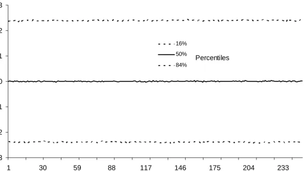
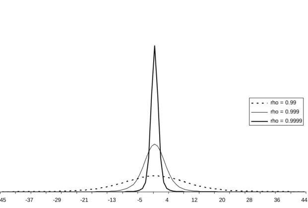
A further understanding of the prior can be obtained through simulation methods. For the sake of brevity, we only present prior simulation results relating to the change in the cointegrating space over time. To facilitate in-terpretation, we present results for then= 2; r= 1case in terms of the angle de…ning the cointegrating space. For the case where T = 250 and = 0:999, Figure 1 plots the median and 16th and 84th percentiles of the prior of the change in this angle between time periods. It can be seen that this prior
density is constant over time (as is implied by Proposition 4) and, hence, our prior implies constant expected change in the cointegrating space. Fur-thermore, = 0:999allows for fairly substantive changes in the cointegrating space over time. That is, it implies that changes in the cointegrating space of one or two degrees each time period are common. For monthly or quarterly data, this would allow for the angle de…ning the cointegrating space to greatly change within a year or two. Figure 2, which plots the entire prior density for the change in this angle for = 0:99, = 0:999and = 0:9999, reinforces this point. Even if we restrict consideration of to values quite near one we are able to allow for large variations in the cointegrating space over time. In fact, = 0:99 allows for implausibly huge changes in the cointegrating space, while = 0:9999 still allows for an appreciable degree of movement in the cointegrating space. Given that our desire is to …nd a state equation which allows for constant gradual evolution in the cointegrating space we accordingly focus on values of which are near to one.2
2.4
An Informative Marginal Prior
The hierarchical prior in (9) is conditionally informative in that it says “this period’s cointegrating space is centered over last period’s”, but marginally is noninformative (i.e. as shown previously, the marginal prior distribution for
pt is Uniform on the Grassmann manifold). However, economic theory often provides us with prior information about the likely location of the cointegrat-ing space. Suppose H is a semi-orthogonal matrix which summarizes such prior information (see Strachan and Inder (2004) or Koop, Strachan, van Dijk and Villani (2006) for examples of how such an H can be constructed and used in standard cointegration models). In this sub-section, we describe how such prior information can be incorporated in our approach. In particular, we want a prior which combines our previous prior which said “ptis centered overpt 1”with the prior information inH and is marginally informative (i.e.
pt has a marginal distribution which is centered overH). We refer to this as an informative marginal prior.
It turns out that such an informative marginal prior can easily be
devel-2This is analogous to the apparently tight priors commonly used for the error covariance
matrix in the state equation of TVP-VAR models. For instance, Primiceri (2005) uses a prior with mean0:0001times the OLS covariance of the VAR coe¢ cients calculated using a training sample. This looks very small but in reality allows for substantial evolution of the VAR coe¢ cients.
oped as a small extension of (9). If we de…ne P = HH0 + H
?H?0 , where 0 1 and use a state equation (now written in terms of the n r
matrices t). t = P t 1 + t (12) t N(0; Inr) fort = 2; :::; T: 1 N(0; 1 1 2Ir P );
where = 11 2 22 ,P =HH0+ H?H?0 , then we have a prior with
attrac-tive properties as formalized in the following proposition.
Proposition 5 If t follows the process de…ned by (12), with j j<1, then: 1. b is N(0; V), where V is de…ned by it variances and covariances (for
t = 1; ::; T): var(bt) = 1 1 2Ir P E(btbt h0 ) = h 1 2Ir P h for h= 2; ::; t 1. 2. E(ptjpt 1) =sp(P t 1).
3. Let be a semi-orthogonal matrix such that sp( ) = E(ptjpt 1). The
following two inequalities hold:
d( ; H) d( t 1; H)
d( ; t 1) d( t 1; H)
4. The mode of the marginal distribution of sp( t) is sp(H).
Proof: See Appendix B.
The fourth property establishes that our prior is an informative marginal prior in the sense de…ned above. To help further interpret this proposi-tion, note that we can write t 1 as the sum of two components: t 1 =
H(H0
t 1) +H?(H?0 t 1). The …rst component is the projection of t 1
H(H0
t 1)+ H?(H?0 t 1). Thus,(P t 1)results from adding the two
com-ponents of t 1 while giving less weight to the projection of t 1 onH?. As
approaches 1, E(ptjpt 1) will approach pt 1 (and the state equation used
previously in (9) is obtained), and approaching0implies that E(ptjpt 1)is
approaching sp(H). In addition, the distance betweensp(H)and sp( t 1)is greater than both d( ; H) and d( ; t 1) and, in this sense, E(ptjpt 1) will
be pulled away from pt 1 in the direction ofsp(H).
In words, the conditional prior of sp( t) given sp t 1 introduced in this sub-section is a weighted average of last period’s cointegrating space (sp t 1 ) and the subjective prior belief about the cointegrating space (sp(H)) and the weights are controlled by .
2.5
Summary
Early on in this section, we set out three desirable qualities that state equa-tions for the time varying cointegrating space model should have. We have now established that our proposed state equations do have these properties. Propositions 1 and 2 establish that (9) implies that the cointegrating space at time t has a distribution which is centered over the cointegrating space at time t 1. Propositions 3 and 4 together with the prior simulation re-sults establish that (9) allows for the change in location of pt from pt 1 to
be small, thus allowing for a gradual evolution of the space comparable to the gradual evolution of parameters which occurs with TVP-VAR models. We have proved that (9) implies that the marginal prior distribution of the cointegrating space is noninformative, but showed how, using the informative marginal prior in (12) the researcher can incorporate subjective prior beliefs about the cointegrating space if desired.
2.6
Bayesian Inference in the Time Varying
Cointe-gration Model
In this section we outline our MCMC algorithm for the time varying cointe-grating space model based on (9). The extension for the informative marginal prior is a trivial one (simply plug the P into the state equation as in (12)). Note that the informative marginal prior depends on the hyperparameter . The researcher can, if desired, treat as an unknown parameter. The ex-tra block to the Gibbs sampler required by this extension is given in Koop, León-González and Strachan (2008b).
We have speci…ed a state space model for the time varying VECM. Our parameters break into three main blocks: the error covariance matrices ( t for all t), the VECM coe¢ cients apart from the cointegrating space (i.e.
( t; 1;t; : : : ; l;t; t) for all t) and the parameters characterizing the cointe-grating space (i.e. t for all t). The algorithm draws all parameters in each block jointly from the conditional posterior density given the other blocks. Standard algorithms exist for providing MCMC draws from all of the blocks and, hence, we will only brie‡y describe them here. We adopt the speci…ca-tion of Primiceri (2005) for t and use his algorithm for producing MCMC draws from the posterior of t conditional on the other parameters. For
( t; 1;t; : : : ; l;t; t)standard algorithms for linear Normal state space mod-els exist which can be used to produce MCMC draws from its conditional posterior. We use the algorithm of Durbin and Koopman (2002). For the third of block of parameters relating to the cointegrating space, we use the parameter augmented Gibbs sampler (see van Dyk and Meng, 2001) devel-oped in Koop, León-González and Strachan (2008a) and the reader is referred to that paper for further details. The structure of this algorithm can be ex-plained by noting that we can replace t 0t in (4) by t t0 where t = t t1 and t = t t where t is a r r symmetric positive de…nite matrix. Note that t is not identi…ed in the likelihood function but the prior we use for t implies that t has a proper prior distribution3 and, thus, is identi…ed under the posterior. Even though t is semi-orthogonal, Koop, León-González and Strachan (2008a) show that the posterior for t has a Normal distribution (conditional on the other parameters). Thus, t can be drawn using any of the standard algorithms for linear Normal state space models, and we use the algorithm of Durbin and Koopman (2002). Then, if desired, the draws of t can be transformed in draws of t or any feature of the cointegrating space. In the traditional VECM, Koop, León-González and Strachan (2008a) pro-vide epro-vidence that this algorithm is very e¢ cient relative to other methods (e.g. Metropolis-Hastings algorithms) and signi…cantly simpli…es the imple-mentation of Bayesian cointegration analysis.
Finally, if (9) is treated as a prior then the researcher can simply select a value for . However, if it is a hierarchical prior and is treated as an unknown parameter, it is simple to add one block to the MCMC algorithm and draw it. In our empirical work, we use a Griddy-Gibbs sampler for this
3The properties of the prior distribution of
tare easily derived from those of the prior
parameter.
Further details on the prior distribution and posterior computations are provided in Appendix A.
3
Application: A Permanent-Transitory
De-composition for In‡ation
In this section, we illustrate our methods using US data from 1953Q1 through 2006Q2 on the unemployment rate (seasonally adjusted civilian unemploy-ment rate, all workers over age 16), ut; interest rate (yield on three month Treasury bill rate), rt;and in‡ation rate (the annual percentage change in a chain-weighted GDP price index), t.4 These variables are commonly-used to
investigate issues relating to monetary policy (e.g. Primiceri, 2005) and we contribute to this discussion but focus on issues relating to cointegration.5 In particular, with cointegration it is common to estimate permanent-transitory variance decompositions which shed insight on the relative roles of permanent and transitory shocks in driving each of the variables. Such issues cannot be investigated with the TVP-VAR methods which are commonly-used with these variables. However, the appropriate policy response to a movement in in‡ation depends upon whether it is permanent or transitory. Thus, our time-varying cointegration methods are potentially useful for policymakers.
An important concern in the day to day practice of monetary policy is whether shocks to in‡ation are transitory or permanent. This can be an im-portant consideration in forecasting and in determining the appropriate pol-icy response. For example, the ratio of transitory volatility to total volatility can be used to weight the recent history of in‡ation for forecasting (see Lans-ing, 2006a). Further, policymakers often focus attention upon movements in core measures of in‡ation as an approximation to permanent changes to in-‡ation6 (see Mishkin, 2007). Recent evidence has suggested that the role of
4The data were obtained from the Federal Reserve Bank of St. Louis website,
http://research.stlouisfed.org/fred2/.
5Note that, by allowing for random walk intercepts, TVP-VARs allow for unit root
behavior in the variables (as does our model). Thus, both approaches allow for perma-nent shocks. Our cointegration-based approach has the additional bene…t that standard methods can be used to carry out a permanent-transitory decomposition.
6It is important to distinguish between permanent movements in in‡ation and
permanent shocks in driving US in‡ation has been decreasing (see Lansing, 2006b). In the application in this section, we shed light on this issue using our time-varying cointegration model. In particular, we show that there has been an increase in the transitory proportion of in‡ation, particularly after 1980. Furthermore, the uncertainty associated with this transitory component has increased also.
We use the time varying VECM in (4) with one lag of di¤erences (l = 1) and a single cointegrating relationship (r = 1). Using the time-invariant version VECM, the BIC selects l = 1and r= 1, which provides support for these choices. We use the state equation for t in (9). Further modelling details and prior choices are given in Appendix A.
We begin by considering measures of the location of the cointegrating space. These are based upon the distance measure d(:; :) in (11), except rather than measure the distance from the last observed space, we measure the distance from a …xed space so as to give an idea of movement in the estimated cointegrating space. That is, we compute d1;t = d( t; H1) where
sp(H1) is a known space with a …xed location. De…ning it in this way, d1;t is bounded between zero and one and is a measure of the distance between
pt =sp( t) and p1 =sp(H1) at timet: A change in the value ofd1;t implies movement in the location of pt.
A limitation of measuring movements in this way is that, while the space
ptmay move signi…cantly, it can stay the same distance fromp1 such thatd1;t does not change. Thus, if we observe no change in d1;t; this does not imply that ptdid not move. This is an unlikely (measure zero) event, but certainly small changes in d1;t do not necessarily indicate the location of pt has not changed very much. A simple solution to this issue is to simultaneously measure the distance from another space p2 = sp(H2) 6= p1. That is, we
compute both d1;t = d( t; H1) and d2;t = d( t; H2). The rationale here
is that if pt moves in such a way that d1;t does not change, then d2;t must change provided p1 6=p2. The rules for interpretation then are quite simple.
If neither d1;t nor d2;t have changed, then pt has not moved. If either d1;t or d2;t or both have changed, then pt has moved. The choices of p1 and p2
are arbitrary. The only necessary condition is that they are not the same. However, movements are likely to be more evident ifp1andp2 are orthogonal
to each other. We choose to setp1to be the space that implies the real interest
rate is stationary andp2 to be the space that implies the unemployment rate
is stationary. That is, for the orderingyt= ( t; ut; rt) then H1 = 2 4 1 0 1 3 5 and H2 = 2 4 0 1 0 3 5:
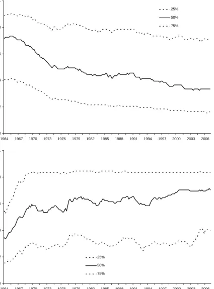
Figure 3 presents plots of the posterior median and the 25th and 75th
percentiles of d1;t and d2;t. It is evident that there has been some movement
in the cointegrating space. In particular, pt is moving towards p1 over the
full sample, whilept has moved away from p2 by 1970 and stayed far from it
for the remainder of the period shown. This suggests the evidence in support of stationary real interest rates has gradually strengthened over time, while the evidence that unemployment is stationary has weakened.
Next, we compute the permanent-transitory variance decomposition for in‡ation using the approach of Centoni and Cubadda (2003). This variance decomposition is a function of the parameters in the VECM. As, in our ap-proach, these parameters vary over time, the computed transitory proportion of in‡ation will vary over time. Figure 4 presents a plot of the posterior me-dian and the 25th and 75th percentiles of the time varying proportion of the variance of in‡ation that is transitory. This …gure shows that the transitory component of in‡ation has historically been low - the median, for example, has always remained below 7%. Permanent shocks, thus, are predominant. But there does appear to have been a slight increase in the size of the tran-sitory component around the middle of the 1980s (as the entire posterior distribution has shifted upwards). Another important observation is the in-crease in the uncertainty associated with the size of the transitory component. That is, the increase in the interquartile range of the posterior shows how it is becoming more dispersed. At all points in time, the 25th percentile is very close to zero (the value which implies that it is only permanent shocks which are driving in‡ation). However the75thpercentile increases noticeably after 1980 as the distribution becomes more dispersed. This rise in the size of the transitory component corresponds roughly with the often-reported fall in total volatility of in‡ation (e.g., Primiceri, 2005).
4
Conclusion
TVP-VARs have become very popular in empirical macroeconomics. In this paper, we have extended such models to allow for cointegration. However, we
have demonstrated that such an extension cannot simply involve adding an extra set of random walk or AR(1) state equations for identi…ed cointegrating vectors. Instead, we have developed a model where the cointegrating space itself evolves over time in a manner which is analogous to the random walk variation used with TVP-VARs. That is, we have developed a state space model which implies that the expected value of the cointegrating space at time t equals the cointegrating space at time t 1. Using methods from the directional statistics literature, we prove this property and other desirable properties of our time varying cointegrating space model.
Posterior simulation can be carried out in the time varying cointegrating space model by combining standard state space algorithms with an algorithm adapted from our previous work with standard (time invariant) VECMs. We also carry out an empirical investigation on a small system of variables commonly used in studies of in‡ation and monetary policy. Our focus is upon how the proportion of in‡ation variability that is transitory has evolved. We …nd that, although permanent shocks are predominant, there has been a slight increase in the transitory component of in‡ation after 1980 and an increase in the uncertainty associated with the estimate of this component.
References
Accardi, L., Cabrera, J. and Watson, G., 1987, Some stationary Markov processes in discrete time for unit vectors, Metron, XLV, 115-133.
Breckling, J., 1989,The Analysis of Directional Time Series: Applications
to Wind Speed and Direction, London: Springer.
Centoni, M. and Cubadda, G., 2003, Measuring the business cycle e¤ects of permanent and transitory shocks in cointegrated time series, Economics Letters, 80, 45-51.
Chikuse, Y., 2003, Statistics on special manifolds, volume 174 ofLecture Notes in Statistics, Springer-Verlag, New York.
Chikuse, Y. 2006, State space models on special manifolds, Journal of
Multivariate Analysis 97, 1284-1294.
Cogley, T. and Sargent, T., 2005, Drifts and volatilities: Monetary poli-cies and outcomes in the post WWII U.S, Review of Economic Dynamics, 8, 262-302.
Downs, T.D., 1972, Orientation statistics,Biometrika 59, 665–676. Durbin, J. and Koopman, S., 2002, A simple and e¢ cient simulation smoother for state space time series analysis, Biometrika, 89, 603-616.
Fisher, N., 1993,Statistical Analysis of Circular Data, Cambridge: Cam-bridge University Press.
Fisher, N. and Lee, A., 1992, Regression models for an angular response,
Biometrics, 48, 665-677.
Fisher, N. and Lee, A., 1994, Time series analysis of circular data,Journal of the Royal Statistical Society, Series B, 56, 327–339.
Godsil, C.D., and Royle, G., 2004, Algebraic Graph Theory, New York: Springer
James, A.T., 1954, Normal multivariate analysis and the orthogonal group,
Annals of Mathematical Statistics, 25, 40–75.
James, A.T., 1964, Distributions of matrix variates and latent roots de-rived from normal samples, Annals of Mathematical Statistics, 35, 475-501.
Johansen, S., 1991, Estimation and hypothesis testing of cointegration vectors in Gaussian vector autoregressive models, Econometrica, 59, 1551-1580.
Khatri, C.G. and Mardia K.V., 1977, The Von Mises-Fisher matrix dis-tribution in orientation statistics, Journal of the Royal Statistical Society. Series B (Methodological), Vol. 39, No. 1., pp. 95-106.
Kass, R. and Raftery, A., 1995, Bayes factors, Journal of the American Statistical Association, 90, 773-795.
Kim, S., Shephard, N. and Chib, S., 1998, Stochastic volatility: likelihood inference and comparison with ARCH models, Review of Economic Studies, 65, 361-93.
Koop, G., León-González, R. and Strachan R.W., 2007, On the evolution of monetary policy, working paper available at
http://personal.strath.ac.uk/gary.koop/koop_leongonzalez_strachan_kls5.pdf. Koop, G., León-González, R. and Strachan, R., 2008a, E¢ cient posterior
simulation for cointegrated models with priors on the cointegration space, forthcoming in Econometric Reviews,
manuscript available at http://personal.strath.ac.uk/gary.koop/.
Koop G., León-González, R. and Strachan R., 2008b, Bayesian inference in a cointegrating panel data model, forthcoming in Advances in Economet-rics,
manuscript available at http://personal.strath.ac.uk/gary.koop/.
Koop, G., Strachan, R., van Dijk, H. and Villani, M., 2006, Bayesian approaches to cointegration, Chapter 25 in The Palgrave Handbook of
Econometrics, Volume 1: Theoretical Econometrics edited by T. Mills
and K. Patterson. Basingstoke: Palgrave-Macmillan.
Krishnaiah, P. and Rao, M., 1961, Remarks on a multivariate Gamma distribution, The American Mathematical Monthly, 68, 342-346.
Lansing, K.J. 2006a, Will moderating growth reduce in‡ation? FRBSF
Economic Letter 2006-37 (December 22).
Lansing, K.J. 2006b, Time-varying U.S. in‡ation dynamics and the new Keynesian Phillips curve, FRBSF Working Paper 2006-15.
Liu, J. and Wu, Y., 1999, Parameter expansion for data augmentation,
Journal of the American Statistical Association, 94, 1264-1274.
Mardia, K. and Jupp, P., 2000,Directional Statistics, Chichester: Wiley. Martins, L. and Bierens, H., 2005, Time varying cointegration, manu-script available at http://econ.la.psu.edu/~hbierens/TVCOINT.PDF.
Mishkin, F., 2007, Headline versus core in‡ation in the conduct of mone-tary policy,Business Cycles, International Transmission and Macroeconomic
Policies Conference, HEC Montreal, Montreal, Canada.
Muirhead, R.J., 1982, Aspects of Multivariate Statistical Theory. New York: Wiley.
Presnell, B., Morrison, S. and Littell, R., 1998, Projected multivariate linear models for directional data, Journal of the American Statistical Asso-ciation, 93, 1068-1077.
Primiceri. G., 2005, Time varying structural vector autoregressions and monetary policy, Review of Economic Studies, 72, 821-852.
Rao, C.R. and Rao, M.B. 1998, Matrix Algebra and its Applications to
Statistics and Econometrics. Singapore: World Scienti…c.
Saikkonen, P. and Choi, I., 2004, Cointegrating smooth transition regres-sions, Econometric Theory, 20, 301— 340.
Strachan, R., 2003, Valid Bayesian estimation of the cointegrating error correction model, Journal of Business and Economic Statistics, 21, 185-195. Strachan, R. and Inder, B. 2004, Bayesian analysis of the error correction model, Journal of Econometrics, 123, 307-325.
Strachan, R. and van Dijk, H., 2007, Valuing structure, model uncer-tainty and model averaging in vector autoregressive processes, Econometric Institute Report EI 2007-11, Erasmus University Rotterdam.
van Dyk, D.A., and Meng, X.L., 2001, The art of data augmentation,
Journal of Computational and Graphical Statistics, 10, 1-111, (with discus-sion).
Villani, M., 2000, Aspects of Bayesian Cointegration. PhD thesis, Uni-versity of Stockholm.
Villani, M., 2005, Bayesian reference analysis of cointegration, Economet-ric Theory, 21, 326-357.
Villani, M., 2006, Bayesian point estimation of the cointegration space,
Appendix A: Posterior Computation and Prior
Dis-tributions
Drawing from the Conditional Mean Parameters Other Than Those De-termining the Cointegration Space
Let us de…ne At = ( t; 1;t; : : : ; l;t; t) where t = t t1 and at =
vec(At) and assume:
at =at 1+ t (13) where t N(0; Q).7 We can rewrite (4) by de…ning zt = t0yt 1 and
Zt = z0t; yt0 1; : : : ; yt l0 ; d0t
0
. Zt is a 1 (k+r) vector where k is the number of deterministic terms plus n times the number of lags. Thus,
yt=AtZt+"t: (14) Vectorizing this equation gives us the form
yt = (Zt0 In)vec(At) +"t or yt = xtat+"t
where xt = (Zt0 In). As we have assumed "t is Normally distributed, the above expression gives us the linear Normal form for the measurement equa-tion for at (conditional on t). This measurement equation along with the state equation (13), specify a standard state space model and the method of Durbin and Koopman (2002) can be used to draw at.
Drawing the Parameters which Determine the Cointegration Space
As in Koop, León-González, and Strachan (2008b), we use the transfor-mations t = t( t) 1 and t = t t where t is ar r symmetric positive de…nite matrix. To show how t can be drawn, we rewrite (4) by de…ning
e yt = yt l X h=1 h;t yt h tdt= t t0yt 1+"t oryet = xetbt +"t
where we have used the relation t t0yt 1 = yt0 1 t bt where bt =
vec( t) and the de…nition ext = yt0 1 t . Again the assumption that "t
7One attractive property of this state equation is that, when combined with (9), it
implies E( tj t 1) = t 1. Moreover, if desired, it is straightforward to adapt this
prior in such a way thatE( tj t 1) = t 1, while all calculations would remain virtually
is Normally distributed gives us a linear Normal form for the measurement equation, this time for bt. This measurement equation along with the state equation, specify a standard state space model and the method of Durbin and Koopman (2002) can be used to drawbt (conditional on the other parameters in the model).
Treatment of Multivariate Stochastic Volatility
In the body of the paper, we did not fully explain our treatment of the measurement error covariance matrix, since it is unimportant for the main theoretical derivations in the paper. Here we provide details on how this is modelled.
We follow Primiceri (2005) and use a triangular reduction of the mea-surement error covariance, t, such that:
t t 0t= t 0t or t= t1 t 0t 1 t 0 ; (15)
where t is a diagonal matrix with diagonal elements j;t for j = 1; ::; p and t is the lower triangular matrix:
t= 2 6 6 6 6 4 1 0 ::: : 0 21;t 1 ::: : : : : ::: : : : : ::: 1 0 p1;t : ::: p(p 1);t 1 3 7 7 7 7 5:
To model evolution in t and t we must specify additional state equa-tions. For t a stochastic volatility framework can be used. In particular, if
t= ( 1;t; ::; p;t)0, hi;t = ln ( i;t),ht = (h1;t; ::; hp;t)0 then Primiceri uses:
ht=ht 1+ut; (16) where ut is N(0; W) and is independent over t and of "t, t and t.
To describe the manner in which tevolves, we …rst stack the unrestricted elements by rows into a p(p2 1) vector as t = 21;t; 31;t; 32;t; ::; p(p 1);t 0. These are allowed to evolve according to the state equation:
where t is N(0; C) and is independent over t and of ut, "t, t and t. We assume the same block diagonal structure for C as in Primiceri (2005).
Prior Distributions
Our model involves four sets of state equations: two associated with the measurement error covariance matrix ((16) and (17)), one for the cointegrat-ing space given in (9) and one for the other conditional mean coe¢ cients (13). The prior for the initial condition for the cointegrating space is already given in (9), and implies a uniform for p1. We now describe the prior for
initial conditions (h0, 0 and a0) and the variances of the errors in the other
three state equations (W, C and Q). We also require a prior for which, inspired by the prior simulation results, we set to being Uniform over a range close to one: 2[0:999;1).
With TVP-VARs it is common to use training sample priors as in, e.g., Cogley and Sargent, 2005, and Primiceri (2005). In this paper we adapt this strategy to the TVP-VECM. Note that for t our prior is identical to Primiceri (2005). Our training sample prior estimates a time-invariant VAR using the …rst ten years of data to choose many of the key prior hyperpara-meters. To be precise, we calculate OLS estimates of the VAR coe¢ cients,
b
A including b, and the error covariance matrix, b and decompose the latter as in (15) to produce b0 and bh0 (where these are both vectors stacking the
free elements as we did with t and ht). We also obtain OLS estimates of the covariance matrices of Ab and b0 which we label VbA and Vb . Using the singular value decomposition b = U SV0, we reorder the elements of U; S;
and V such that the diagonal elements of S are in descending order. We then set the elements of ba0 corresponding to b to be the …rst r columns of
U S. Next, de…neVr to be the …rstr columns ofV:We pre-multiply the rows of VbA corresponding to b by (Vr0 I) and post-multiply the corresponding columns of VbA by(Vr I):
Using these, we construct the priors for the initial conditions in each of our state equations as:
a0 N ba0;4Vb ;
0 N b0;4Vb
and
Next we describe the priors for the error variances in the state equations. We follow the common practice of using Wishart priors for the error precision matrices in the state equations:
Q 1 W Q; Q 1 (18)
For (18) we set Q = 40 and Q= 0:0001Vb . ForW 1:
W 1 W W; W 1 (19)
with W = 4 and W = 0:0001In.
We adopt the block-diagonal structure for C given in Primiceri (2005). Call the two blocks C1 and C2. We use a Wishart prior for Cj 1:
Cj 1 W Cj; Cj1 :
with C1 = 2; C2 = 3and Cj = 0:01Vb j forj = 1;2and Vb j is the block cor-responding to Cj taken fromVb . See Primiceri (2005) for further discussion and motivation for these choices.
These values are either identical or (where not directly comparable due to our having a VECM) similar in spirit to those used in Primiceri (2005) and Cogley and Sargent (2005).
Remaining Details of Posterior Simulation
The blocks in our algorithm for producing draws of bt, at have already been provided. Here we discuss the other blocks of our MCMC algorithm. In particular, we describe how to draw from the full posterior conditionals for the remaining two sets of state equations, the covariance matrices of the errors in the state equations and . Since most of these involve standard algorithms, we do not provide much detail. As in Primiceri (2005), draws of t can be obtained using the algorithm of Durbin and Koopman (2002) and draws of ht using the algorithm of Kim, Shephard and Chib (1998).
The conditional posteriors for the state equation error variances begin with:
Q 1jData W Q; Q
1
where
and Q 1 = " Q+ T X t=1 (at at 1) (at at 1)0 # 1 : Next we have: W 1jData W W; W 1 where W =T + W and W 1 = " W + T X t=1 (ht ht 1) (ht ht 1)0 # 1 :
The posterior for Cj 1 (conditional on the states) is then Wishart:
Cj 1jData W Cj; C 1 j where Cj =T + Cj and Cj1 = " Cj + T X t=1 a(tj+1) a(tj) a(tj+1) a(tj) 0 # 1
and a(tj) are the elements ofat corresponding toCj.
The posterior for is non-standard due to the nonlinear way in which it enters the distribution for the initial condition for b1 in (9). We therefore draw this scalar using a Griddy-Gibbs algorithm based on our Uniform prior. In our empirical work, we run our sampler for 8000 burn-in replications and then include the next 16000 replications.
Appendix B: Proofs
Proof of Proposition 1: We will show that the density ofptconditional on ( t; t 1; t 1) is maximized at pt = sp( t 1) for any value of ( t; t 1).
This proves that the density ofptconditional on( t 1; t 1)is also maximized
at pt = sp( t 1). Clearly, the mode is also the same if we do not condition
on t 1.
The state equation in (9) implies that the conditional density of t given t 1 is matric Normal with mean t 1 and covariance matrix Inr: Thus, using Lemma 1.5.2 in Chikuse (2003), it can be shown that the implied dis-tribution for tj( t; t 1; t 1) is the matrix Langevin (or von Mises–Fisher)
distribution denoted by L n; r; ~F (Chikuse, 2003, p. 31), where
~
F = t 1 t = t 1 t 1 t
The form of the density function for L n; r; ~F is given by
f t( tjF~) =
expntr( ~F0
t)
o
0F1 n2;14F~0F~
Recall that Pt= t 0t. The density function fPt(Pt) of Pt, conditional on F~,
can be derived from the density function f t( t) of t using Theorem 2.4.8 in Chikuse (2003, p. 46): fPt(Pt) =AL Z Or exp(trF~0 tQ)[dQ] =AL 0F1( 1 2r; 1 4 ~ F0PtF~)
where AL is a constant not depending onPt (AL1 = 0F1(12n;14F~0F~)) and Or is the orthogonal group of r r orthogonal matrices (Chikuse (2003), p. 8). Note that we have used the integral representation of the0F1 hypergeometric
function (Muirhead, 1982, p. 262). Khatri and Mardia (1976, p. 96) show that 0F1(12r;14F~0PtF~) is equal to 0F1(12r;14Gt), where Gt = diag(g1; :::; gr) is an r r diagonal matrix containing the singular values of F~0P
tF~. We …rst show that0F1(12r;14Gt)is an increasing function of each of the singular values
gi, for each i = 1; :::; r. We then show that each of these singular values is maximized when 0t 1Pt t 1 = Ir. Note that 0t 1Pt t 1 = Ir implies that the distance between sp( t) and sp( t 1), as de…ned in Larsson and Villani (2001), is zero and thus pt =sp( t 1).
We …rst show that the following standard expression for0F1(12r;14Gt)(e.g. Muirhead, 1982, p. 262): 0F1( 1 2r; 1 4Gt) = Z O(r) exp( r X i=1 pg iqii)[dQ]
with Q=fqijg, is equivalent to:
0F1( 1 2r; 1 4Gt) = Z ~ Or r Y i=1 (exp(pgiqii) +exp( pgiqii))[dQ] (20)
whereO~(r)is a subset ofO(r)consisting of matricesQ2O(r)whose diagonal elements are positive. This equivalence can be noted by writing:
Z O(r) exp( r X i=1 pg iqii)[dQ] = Z fO(r):q11 0g exp( r X i=1 pg iqii)[dQ]+ Z fO(r):q11<0g exp( r X i=1 pg iqii)[dQ]
The second integral in the sum can be rewritten by making a change of variables from Q to Z, where Z results from multiplying the …rst row of
Q by ( 1). Note that Z results from pre-multiplying Q by an orthogonal matrix and thus Z still belongs to O(r) and the Jacobian is one (Muirhead, 1982, Theorem 2.1.4). Thus, the second integral in the sum can be written as: Z fO(r):q11<0g exp( r X i=1 pg iqii)[dQ] = Z fO(r):z11 0g exp( pgiz11) exp( r X i=2 pg izii)[dZ] = Z fO(r):q11 0g exp( pgiq11) exp( r X i=2 pg iqii)[dQ] Thus: Z O(r) exp( r X i=1 pg iqii)[dQ] = Z fO(r):q11 0g
(exp(pgiq11)+exp( pgiq11)) exp(
r
X
i=2
pg
iqii)[dQ]
Doing analogous changes of variables for the other rows, we arrive at equation (20). Note that the function exp(cx) + exp( cx) is an increasing function of
x when both x and care positive. Thus, from expression (20), 0F1(12r;14Gt) is an increasing function of each of the singular valuesgi, for eachi= 1; :::; r.
Let us now see that each of the singular values of F~0P
tF~ is maximized when 0t 1Pt t 1 =Ir. WriteF~ = t 1C, whereC = t 1 tis ar rmatrix. Let t? be the orthogonal complement of t (i.e. ( t; t?) is an (n n) orthogonal matrix) andPt?= t? 0t?. Note thatPt+Pt? =In(becausePt+
Pt? = ( t; t?)( t; t?)0 = Ir). Thus, C0 0t 1Pt t 1C +C0 0t 1Pt? t 1C =
C0C. Let (a
1; ::; ar) be the singular values of A = C0 0t 1Pt t 1C, with
(a1 a2 ::: ar 0). Similarly, let (b1; ::; br) be the singular values of
B =C0 0t 1Pt? t 1C(ordered also from high to low). Similarly, let(c1; ::; cr) be the singular values of(C0C). BecauseA; B;(C0C)are positive semide…nite
and symmetric, eigenvalues and singular values coincide. Thus, Proposition 10.1.1 in Rao and Rao (1998, p. 322) applies, which implies that: a1+br
c1; a2 +br c2; a3 +br c3,...,ar +br cr. Since br 0 this implies
a1 c1; a2 c2; a3 c3,...,ar cr. Note that if 0t 1Pt t 1 = Ir then
A = C0C and so a1 = c1; a2 = c2; a3 = c3,...,ar = cr. Thus, each of the singular values of F~0P
Proof of Proposition 2:
We will proof that E(ptj( t; t 1; t 1)) = sp( t 1). Note that this
proves that E(ptj( t 1; t 1)) = sp( t 1), because if = t 1 minimizes
E(d2(
t; )j( t; t 1; t 1))for every t, it will also minimizeE(d2( t; )j( t 1; t 1)).
Similarly, it also proves that E(ptj t 1) =sp( t 1).
Recall that tj( t; t 1; t 1)follows a Langevin distributionL n; r; ~F ,
with F~ = t 1 t = t 1 t 1 t. Let G = t t 1 and write G using
its singular value decomposition as G = OM P0, where O and P are r r orthogonal matrices, and M is an r r diagonal matrix. Hence, F~ =
t 1P M O0. Write F~ = t 1P M O0 = M O0, where = t 1P. SinceP is a
r rorthogonal matrix,sp( t 1) =sp( ). We will prove thatE(pt) = sp( ). In order to prove this, we will prove thatE( t 0t) = U DU0, withU = ( ;
?),
where ? is the orthogonal complement of , and D = fdijg is a diagonal matrix with d11 d22 ::: dnn. De…ne the n r matrix Z = U0 tO, so that E( t 0t) =U E(ZO0OZ0)U0 =U E(ZZ0)U0. Let Z =fz
ijg.
The distribution of Z0 is the same as the distribution of the matrix that
Khatri and Mardia (1977) denote as Y at the bottom of page 97 of their paper. They show, in page 98, that E(zijzkl) = 0 for all i; j; k; lexcept when (a) i = k = j = l, i = 1;2; :::; r; (b) i = k, j = l (i 6= j); (c) i = j, k = l
(i6=k); (d) i=l, j =k (i6=j),i; j = 1;2; :::; r. Note that the (i; k)element of ZZ0 is Pr
h=1zihzkh. Thus,E(ZZ0) is a diagonal matrix and we can write
E( 0) = U DU0, where D=E(ZZ0).
To …nish the proof we need to show that each of the …rst r values in the diagonal of D=E(ZZ0) is at least as large as any of the othern r values.
The Jacobian from t to Z is one (Muirhead, 1982, Theorem 2.1.4), and hence the density function of Z is:
ALexp(tr(MZ~)) = ALexp( r
X
l=1
(mlz~ll))
where Z~ =fz~ijg consists of the …rst r rows of Z, M =diag(m1; :::; mr) and
AL is a normalizing constant. If we let Z^ =fz^ijg be the other n r rows, what needs to be proved can be written as: E(Prl=1(~zjl)2) E(
Pr
l=1(^zpl)2) for any j; p such that 1 j r, 1 p n r.
Note that (Prl=1(~zjl)2) is the euclidean norm of the jth row of Z and similarly Prl=1(^zpl)2 is the norm of the (r+p)th row ofZ. Let S1 be de…ned
than the (r+p)th row. Let S
2 be the set of semi-orthogonal matrices where
the opposite happens. Thus, E(Prl=1(~zjl)2) can be written as the following sum of integrals: AL Z S1 ( r X l=1 (~zjl)2) exp ( r X l=1 mlz~ll ) [dZ]+AL Z S2 ( r X l=1 (~zjl)2) exp ( r X l=1 mlz~ll ) [dZ]
where [dZ] is the normalized invariant measure on the Stiefel manifold (e.g. Chikuse, 2003, p. 18). Now note that:
AL Z S2 ( r X l=1 (~zjl)2) exp ( r X l=1 mlz~ll ) [dZ] =AL Z S1 ( r X l=1 (^zpl)2) exp ( mjz^pj+ r X l=1;l6=j mlz~ll ) [dZ]
This equality can be obtained by making a change of variables from Z toQ
where Qresults from swapping thejth and (r+p)th rows ofZ. Note thatQ is also semi-orthogonal, and that because the transformation involves simply swapping the position of variables, the Jacobian is one. Thus,E(Prl=1(~zjl)2) can be written as:
AL Z S1 ( r X l=1 (~zjl)2) exp ( r X l=1 mlz~ll ) [dZ]+AL Z S1 ( r X l=1 (^zpl)2) exp ( mjz^pj+ r X l=1;l6=j mlz~ll ) [dZ]
Similarly, E(Prl=1(^zpl)2) can be written as:
AL Z S1 ( r X l=1 (^zpl)2) exp ( r X l=1 mlz~ll ) [dZ]+AL Z S1 ( r X l=1 (~zjl)2) exp ( mjz^pj+ r X l=1;l6=j mlz~ll ) [dZ] Thus, E(Prl=1(~zjl)2) E( Pr l=1(^zpl) 2) is equal to: AL Z S1 ( r X l=1 (~zjl)2 r X l=1 (^zjl)2) exp ( r X l=1 mlz~ll ) exp ( mjz^pj+ r X l=1;l6=j mlz~ll )! [dZ]
Following Chikuse (2003, p. 17), we can make a change of variables Z =
W N, where W is a n r semi-orthogonal matrix that represents an element in the Grassmann manifold, and N is an r r orthogonal matrix. That is, W is seen as an element of the Grassmann manifold of planes (Gr;n r) and N is an element of the orthogonal group of r r orthogonal matrices
(O(r)). The measure [dZ] can be written as [dZ] = [dW][dN], where [dN]
is the normalized invariant measure in O(r)and [dW] is another normalized measure whose expression can be found in Chiku