Impedance Tomography
Emma Rosa Malone
A dissertation submitted in partial fulfillment of the requirements for the degree of
Doctor of Philosophy of
University College London.
Department of Medical Physics and Biomedical Engineering University College London
Author Declaration
I, Emma Rosa Malone, confirm that the work presented in this thesis is my own. Where information has been derived from other sources, I confirm that this has been indicated in the work.
Multifrequency Electrical Impedance Tomography (MFEIT) is an emerging imaging modality which exploits the dependence of tissue impedance on frequency to recover images of conductivity. Given the low cost and portability of EIT scanners, MFEIT could provide emergency diagnosis of pathologies such as acute stroke, brain injury and breast cancer. Whereas time-difference, or dynamic, EIT is an established technique for monitoring lung ventilation, MFEIT has received less attention in the literature, and the imaging methodology is at an early stage of development. MFEIT holds the unique potential to form images from static data, but high sensitivity to noise and modelling errors must be overcome.
The subject of this doctoral thesis is the investigation of novel techniques for including spectral information in the image reconstruction process. The aim is to improve the ill-posedness of the inverse problem and deliver the first imaging methodology with sufficient robustness for clinical application. First, a simple linear model for the conductivity is defined and a simultaneous multifrequency method is developed. Second, the method is applied to a realistic numerical model of a human head, and the robustness to modelling errors is investigated. Third, a combined image reconstruction and classification method is developed, which allows for the simultaneous recovery of the conductivity and the spectral information by introducing a Gaussian-mixture model for the conductivity. Finally, a graph-cut image segmentation technique is integrated in the imaging method. In conclusion, this work identifies spectral information as a key resource for producing MFEIT images and points to a new direction for the development of MFEIT algorithms.
Acknowledgements
It has been a great privilege to work with my principle supervisor, Simon Arridge, who has provided me with unfaltering intellectual and moral support throughout my doctoral studies. I am grateful to David Holder for introducing me to the topic of my dissertation, and Timo Betcke for many helpful discussions.
I extend my thanks to Gustavo Sato Dos Santos, Markus Jehl, Jem Hebden, Gary Royle, Ben Cox, Bruce Amm, David Davenport, and to my colleagues in both the EIT group and CMIC, each of whom have provided me with significant assistance and support as I undertook this work.
I am grateful to my PhD examiners Ville Kolehmainen and Dean Barratt for their many valuable comments.
Finally, I wish to thank my parents Sinéad and Patrick, my siblings Hannah and Stephen, my partner Sam, and my friends for their limitless patience and encouragement.
This work was funded by the EPSRC grant EP/J50225X/1.
1 Overview 15 1.1 Introduction . . . 15 1.2 Purpose . . . 18 1.3 Structure . . . 19 1.4 Publications . . . 19 2 Literature review 21 2.1 Introduction . . . 21 2.1.1 Bioimpedance . . . 21 2.1.2 EIT measurements . . . 23
2.1.3 EIT imaging modalities . . . 25
2.1.4 EIT of the human head . . . 27
2.2 Image reconstruction principles . . . 32
2.2.1 Introduction . . . 32
2.2.2 Ill-posedeness . . . 33
2.3 Mathematical problem definition of EIT . . . 34
2.4 Forward problem . . . 36
2.4.1 Weak formulation . . . 37
2.4.2 Numerical methods . . . 37
2.4.3 Mesh generation . . . 38
2.4.4 Electrode model . . . 39
2.4.5 Galerkin FEM formulation . . . 40
2.4.6 Sensitivity matrix . . . 42
2.5 Inverse problem . . . 43
2.5.1 Introduction . . . 43
2.5.2 Regularization . . . 44
2.5.3 Linear algorithms . . . 45
Contents 6
2.5.5 Nonlinear direct methods . . . 53
2.5.6 Other methods . . . 55
2.5.7 Regularization parameter selection . . . 56
2.6 Multifrequency EIT . . . 57
2.6.1 Introduction . . . 57
2.6.2 Simple frequency-difference . . . 58
2.6.3 Weighted frequency difference . . . 58
2.7 Image segmentation . . . 60
2.7.1 Introduction . . . 60
2.7.2 Labelling problem with MRF prior . . . 60
2.7.3 Graph cut optimization . . . 61
3 Multifrequency EIT using spectral constraints 64 3.1 Introduction . . . 64 3.1.1 Overview . . . 64 3.1.2 Related work . . . 64 3.1.3 Purpose . . . 65 3.1.4 Experimental design . . . 65 3.2 Methods . . . 66 3.2.1 Fraction model . . . 66
3.2.2 Fraction image reconstruction . . . 68
3.2.3 Fraction image reconstruction: indirect method . . . 72
3.2.4 Image quantification . . . 73
3.3 Results . . . 74
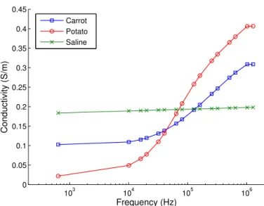
3.3.1 Tissue impedance spectra . . . 74
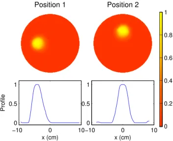
3.3.2 Numerical Validation . . . 74
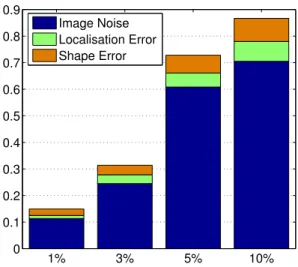
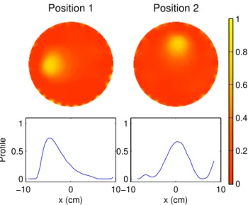
3.3.3 Robustness to spectral errors . . . 75
3.3.4 Phantom study . . . 78
3.3.5 Comparison with indirect multifrequency imaging . . . 79
3.3.6 Comparison with WFD conductivity imaging . . . 81
3.3.7 Spectral constraints method for nonlinear case . . . 81
3.3.8 Multiple tissue case . . . 82
3.3.9 Approximation error evaluation . . . 84
3.4.1 Robustness to spectral errors . . . 88
3.4.2 Comparison with indirect multifrequency imaging . . . 88
3.4.3 Comparison with WFD conductivity imaging . . . 89
3.4.4 Multiple tissue case . . . 89
3.4.5 Approximation error evaluation . . . 90
3.5 Conclusion . . . 90
4 Stroke type differentiation using spectrally constrained MFEIT 92 4.1 Introduction . . . 92 4.1.1 Overview . . . 92 4.1.2 Related work . . . 92 4.1.3 Purpose . . . 93 4.1.4 Experimental design . . . 93 4.2 Methods . . . 95
4.2.1 Model and tissue impedance spectra . . . 95
4.2.2 Data simulation . . . 96 4.2.3 Image reconstruction . . . 97 4.2.4 Numerical validation . . . 97 4.2.5 Error simulation . . . 98 4.2.6 Image quantification . . . 98 4.3 Results . . . 99 4.3.1 Numerical validation . . . 99
4.3.2 Erroneous electrode positions . . . 100
4.3.3 Erroneous tissue spectra . . . 100
4.3.4 Erroneous electrode impedances . . . 101
4.4 Discussion . . . 105
4.4.1 Numerical validation . . . 105
4.4.2 Erroneous electrode positions . . . 105
4.4.3 Erroneous tissue spectra . . . 105
4.4.4 Erroneous electrode impedances . . . 106
4.4.5 Technical remarks . . . 106
4.5 Conclusion . . . 107
5 A reconstruction-classification method for MFEIT 108 5.1 Introduction . . . 108
Contents 8 5.1.1 Overview . . . 108 5.1.2 Related work . . . 108 5.1.3 Purpose . . . 109 5.1.4 Experimental design . . . 109 5.2 Method . . . 111 5.2.1 Multinomial model . . . 111
5.2.2 Combined reconstruction-classification outline . . . 112
5.2.3 Reconstruction . . . 113
5.2.4 Classification . . . 114
5.2.5 Frequency-difference reconstruction-classification outline . . . 116
5.2.6 Frequency-difference reconstruction . . . 117
5.2.7 Frequency-difference classification . . . 118
5.2.8 Spatial smoothing . . . 118
5.2.9 Image quality evaluation . . . 118
5.3 Results . . . 119
5.3.1 Numerical phantom and data simulation . . . 119
5.3.2 RC with homogeneous MRF regularization . . . 119
5.3.3 Robustness to spectral errors . . . 120
5.3.4 RC with independent elements . . . 121
5.3.5 RC with label-dependant MRF regularization . . . 121
5.3.6 Frequency-difference RC: numerical validation . . . 121
5.3.7 Image quality evaluation . . . 122
5.3.8 Comparison with other methods . . . 122
5.3.9 Phantom experiment . . . 123
5.4 Discussion . . . 133
5.4.1 Numerical results . . . 133
5.4.2 Robustness to spectral errors . . . 133
5.4.3 Frequency-difference combined reconstruction-classification . . . 133
5.4.4 Comparison with other methods . . . 134
5.4.5 Phantom experiment . . . 135
5.5 Conclusion . . . 135
6 Reconstruction-classification using graph cut optimization 137 6.1 Introduction . . . 137
6.1.1 Overview . . . 137
6.1.2 Related work . . . 137
6.1.3 Purpose . . . 138
6.1.4 Experimental design . . . 138
6.2 Method . . . 138
6.2.1 Bayesian formulation of the inverse problem of EIT . . . 139
6.2.2 Labelling in MFEIT . . . 139
6.2.3 Hidden Markov Random field model . . . 140
6.2.4 Gaussian HMRF model . . . 140
6.2.5 Gaussian HMRF model-based labelling in MFEIT . . . 141
6.2.6 Reconstruction-classification with HMRF: outline . . . 142
6.2.7 Reconstruction . . . 143
6.2.8 Labelling with graph-cut optimization . . . 143
6.2.9 Classification: fitting the HMRF model with EM . . . 144
6.3 Results . . . 146
6.3.1 Numerical validation . . . 146
6.3.2 Robustness to spectral errors . . . 146
6.3.3 Phantom experiment . . . 146
6.4 Discussion . . . 151
6.4.1 Methodology . . . 151
6.4.2 Numerical validation . . . 151
6.4.3 Robustness to spectral errors . . . 152
6.4.4 Phantom experiment . . . 152
6.5 Conclusion . . . 152
7 Conclusion 154 7.1 Summary of findings . . . 154
7.2 Limitations and future work . . . 156
7.2.1 Conductivity modelling . . . 156
7.2.2 Boundary modelling errors . . . 157
7.2.3 Algorithm speed . . . 158
List of Figures
2.1 Cole-Cole model of electrical properties of a cell. . . 22
2.2 The movement of current through cells at low and high frequencies. . . 22
2.3 The UCL Mk 2.5 EIT system. . . 23
2.4 Diagram of the two-electrode and four-electrode measurement methods. 23 2.5 Conductivity of tissues in the head. . . 28
2.6 Binary image segmentation example. . . 61
2.7 Schematic of graph cut optimization method. . . 62
3.1 Direct and indirect fraction reconstruction. . . 73
3.2 Conductivity values of test tissues. . . 75
3.3 Fraction reconstruction numerical validation model. . . 76
3.4 Fraction reconstruction numerical validation images. . . 76
3.5 Robustness to spectral errors images. . . 77
3.6 Robustness to spectral errors image quantification. . . 78
3.7 Phantom experiment setup. . . 78
3.8 Phantom experiment fraction images. . . 79
3.9 Absolute conductivity images of phantom. . . 80
3.10 Indirect multifrequency imaging results. . . 80
3.11 Image quantification for absolute conductivity and fraction images. . . . 81
3.12 WFD conductivity images of phantom. . . 82
3.13 Image quantification for WFD conductivity and fraction images. . . 82
3.14 WFD comparison simulation model. . . 83
3.15 WFD comparison simulation fraction images. . . 83
3.16 WFD comparison simulation conductivity images. . . 84
3.17 Four-tissue case tissue spectra. . . 85
3.18 Four-tissue case numerical model. . . 85
3.19 Four-tissue case fraction images. . . 86
3.20 Approximation error evaluation model. . . 86
4.1 Conductivity spectra of tissues in the head. . . 96
4.2 Human head model. . . 96
4.3 Numerical validation imaging results. . . 99
4.4 Numerical validation image quantification results. . . 99
4.5 Electrode areas for the fine and coarse meshes. . . 100
4.6 Erroneous electrode positions imaging results. . . 101
4.7 Erroneous electrode positions image quantification results. . . 101
4.8 Erroneous tissue spectra imaging results. . . 102
4.9 Erroneous tissue spectra image quantification results. . . 102
4.10 Frequency-difference conductivity spectra of tissues in the head. . . 103
4.11 Erroneous conductivity spectra imaging results. . . 104
4.12 Erroneous conductivity spectra image quantification results. . . 104
5.1 Numerical phantom model. . . 120
5.2 Reconstruction-classification with homogeneous MRF. . . 124
5.3 Robustness to errors in the initial guess of the tissue spectra. . . 125
5.4 Reconstruction-classification in the case of independent elements. . . 126
5.5 Reconstruction-classification with label-dependent MRF. . . 127
5.6 Frequency-difference reconstruction-classification model. . . 128
5.7 Frequency-difference reconstruction-classification results. . . 129
5.8 Image quality of numerical results. . . 130
5.9 Comparison with other methods. . . 130
5.10 Phantom experiment setup and RC results for absolute data. . . 131
5.11 Phantom experiment RC results for frequency-difference data. . . 132
6.1 Schematic representation of the prior models used in RC. . . 141
6.2 Reconstruction-classification with graph cuts, numerical validation. . . . 147
6.3 Reconstruction-classification with graph cuts, image quantification. . . . 148
6.4 Robustness to errors in the initial guess of the tissue spectra. . . 149
List of symbols
Chapter 2 Symbol Description Z Impedance R Resistance C Capacitance ω Frequency I Current V Voltage L Number of electrodes l Electrode index v Voltage measurements p(x) Probability of xL(x,y) Negative log-likelihood of ygiven x
A Forward map
Ψ Regularization function
τ Regularization parameter h Measurement noise Σy Covariance of y
Ω Parameter space domain
∂Ω Parameter space boundary
γ Admittivity σ Conductivity Permittivity E Electric field J Current density D Electric displacement H Magnetic flux B Magnetic field
ν Permeability
ρ Electric charge density n Outward normal unit vector
z Contact impedance
P Number of current injection patterns
p Current pattern index
Q Number of measurement pairs
q Measurement pair index
K Number of measurements k Measurement index M Number of nodes N Number of elements n Element index Φ Objective function
J Jacobian of the forward map ∇Φ Gradient of the objective function ∇2Φ Hessian of the objective function
d Search direction
α Step size T Labels space V Voxels space
X Image labellings space
Chapter 3 Symbol Description M Number of frequencies i Frequency index J Number of tissues j Tissue index
ij Conductivity of tissue j at frequencyi fnj Fraction of element n and tissuej
List of Figures 14
Chapter 5
Symbol Description
ζnj Class/tissue labels λj Class probability mj Class spectrum mean
Σj Class spectrum variance
Γj Class parameter of the NIW distribution
νj Class parameter of the NIW distribution θj The pair (mj,Σj)
σ Conductivity matrix of values σni, sizeN×M
v Data matrix of values vki, sizeK×M
ρni Reconstruction auxiliary variable ρni= logσni rnj Responsibility
Chapter 6
Symbol Description
Overview
1.1
Introduction
Electrical Impedance Tomography (EIT) is a non-invasive technique for imaging phys-iological and pathological body functions. The underlying principle is to exploit the electrical properties of biological tissues to extract information about the anatomy and physiology of organs. A small amount of current is injected into the body and voltage measurements are acquired using peripheral electrodes. A reconstruction algorithm based on a modified formulation of Ohm’s law for current flow in a volume is implemented to image the impedance distribution of the subject in two or three dimensions.
If current travelled in a straight, collimated beam between source and sink, then an image of conductivity could be reconstructed using a simple backprojection algorithm, in the same way as for Computed Tomography. Only the conductive tissue crossed by the current would contribute to the measurements, therefore the information contained in the measurements could be spread back along the localized current flow path. In reality, although the current density is higher near the electrodes, the current flows in the whole object, and the spatial information provided by the measurements is poor. By mapping the current density in the domain, a measure of the sensitivity of the data to changes in conductivity in different locations is obtained. This provides an indication for each injection pattern of where to "place" the information contained in the measurements, which must be spread out unevenly across the domain. Most commonly used EIT reconstruction algorithms are based on sensitivity mapping (see section 2.5). In this sense EIT is non-local, and all voxels and measurements must be considered at the same time in order to reconstruct an image. Despite the name, EIT is also non-tomographic, in that slices cannot be reconstructed independently. Furthermore, EIT is severely ill-posed because small errors in the measurements can produce large errors in the reconstructed image (see section 2.2.2). From the mathematical point of
1.1. Introduction 16
view, this makes EIT an interesting and challenging imaging problem.
The problem of determining the conditions under which the internal conductivity of an object can be uniquely determined from boundary voltage measurements was first studied by Calderoń in 1980 [22] for the linearized problem (see section 2.4). In principle, if the boundary shape is known exactly, the current-to-voltage map depends uniquely on conductivity. Thus, the conductivity can be determined by full knowledge of the current-to-voltage map on the entire boundary. In practice, knowledge of the boundary is incomplete and uncertain, and the reconstruction depends strongly on modelling errors such as boundary geometry, electrode placement, size and shape, and contact impedance of the interface between the electrode and the skin.
Imaging a small and localized change in conductivity, which occurs over time, con-stitutes a relatively simple problem (see section 2.1.3.1). Two data sets are acquired at different time points and then subtracted. In this case, the relationship between conductivity and voltage changes is often modelled by a linearized model, and the conductivity change can be recovered by inverting the sensitivity map (see section 2.5.3). Producing one-shot static images without baseline measurements, is an exponentially more difficult problem. The first reason is that the data do not, in general, depend linearly on conductivity. Some attempts have been made to solve the full nonlinear problem and recover an image of the absolute conductivity values from a single data set (see sections 2.1.3.2 and 2.5.4) [62, 113]. However, a consequence of the problem being ill-posed is that it is much easier to image a change in conductivity, than its absolute value: when two data sets are subtracted, constant modelling or instrumentation errors are cancelled out, whereas if the absolute data is used, the reconstruction is more sensitive to errors. For this reason, the overwhelming majority of clinical EIT images have been produced using time-difference imaging.
The difficulty in imaging absolute conductivity has prompted researchers to investigate multifrequency methods for producing static images. Multifrequency EIT (MFEIT) involves varying the modulation frequency of the injected current, and acquiring two or more data sets at different frequencies (see section 2.6). The conductivity spectrum of biological tissues is dependent on histology; therefore it is possible to distinguish between tissues on the basis of their frequency response. Following the same logic of time-difference imaging, it seems natural to attempt to image a variation of conductivity across frequency: i.e. use a low frequency as reference and subtract two data sets acquired at different frequencies; then reconstruct an image by inverting the sensitivity
map calculated at the reference frequency. Unfortunately this approach is successful only in resolving a small, frequency dependent anomaly from a frequency independent, homogeneous background [97, 58, 3, 83]. The method has been extended to the case of a frequency dependent background by using a weighted difference between the data, but the range of applications remains severely limited. This technique is unsuitable for clinical application in that it does not accommodate for the complexity of human anatomy.
Initially developed for geophysical studies, EIT was first applied to clinical research in 1987 by the Sheffield University research group, led by Barber and Seagar in the Department of Medical Physics and Clinical Engineering at Royal Hallamshire Hospital. The Sheffield Mark 1 EIT system had a ring of 16 electrodes, and a single current source [17]. Using a multiplexer, current was injected and voltages were measured at adjacent pairs of electrodes. Most early clinical studies were made with the Sheffield Mark I, and many research groups still use systems based on this first example (see section 2.1.2) [72, 82, 26, 35]. The first algorithm for imaging conductivity changes in a 2D cross-section, the so-called "Sheffield algorithm", was based on a backprojection method [6]. The Sheffield group is also accredited with proposing to reference measurements taken at different frequencies against each other [16, 41]. Three-dimensional imaging methods and realistic electrode models were initially developed at the Rensselaer Polytechnic Institute [23, 104, 74], and statistical approaches to image reconstruction and regularization were pioneered by researchers at the Universities of Helsinki and Kuopio (now University of Eastern Finland) [111, 113, 59, 60]. Electrical Impedance and Diffuse Optical Reconstruction Software (EIDORS) is a freely available MATLAB toolbox for EIT imaging [86, 66] based on software developed at the Universities of Manchester and Kuopio [114, 112].
The benefits of EIT applications in medicine lie in the possibility of obtaining high temporal resolution, and in the portability and limited cost of the scanner. The main limitation is the low spatial resolution, which is due to the non-locality and high sensitivity of the reconstruction problem to modelling and experimental errors. EIT has been applied successfully in clinical studies to monitor dynamic body functions such as lung ventilation [74], gastric emptying [70] and the cardiac cycle [34]. Holder proposed EIT as a method for imaging neuronal depolarization [47] and localizing epileptic foci in the brain [48] (see section 2.1.4.2).
EIT is currently being investigated as a clinical diagnostic tool. The applications listed previously all involve imaging of a time series, and therefore time-difference methods
1.2. Purpose 18
are used. In order to extend the application of EIT to diagnostic imaging, a method for producing static images is necessary. For example, it has been proposed to use MFEIT for breast cancer screening [69], lung imaging [41, 18], monitoring of brain injury in intensive care [99] and differentiating between stroke types in the ambulance (see section 2.1.4.1) [52, 92, 83]. The latter techniques all involve the differentiation of tissues on the basis of their characteristic impedance spectrum, therefore it is sufficient to acquire a single multifrequency dataset. However, MFEIT has received little attention in the literature and is at an earlier stage of development with respect to time-difference EIT. Due to the ill-posedness of the inverse problem, MFEIT imaging is highly sensitive to modelling errors and suffers from poor signal-to-noise ratio. The main challenge in this field is to develop an imaging approach with sufficient robustness to noise and model uncertainty for clinical application.
1.2
Purpose
The subject of this dissertation is the investigation of novel approaches to multifrequency EIT for diagnostic purposes, with a focus on brain imaging. The ultimate goal of this work is to provide a mathematical framework for static EIT imaging for a multitude of clinical applications. The use of multifrequency data and prior spectral information is explored as a means to improve the ill-posedness of the image reconstruction problem, and thus improve the outcome of the solution. The purpose is to provide an algorithm with sufficient robustness to experimental error and model uncertainty to be applied reliably to clinical data. The main contributions to the field are summarized as follows:
• The proposal of a novel method for performing MFEIT using explicit spectral constraints, thefraction reconstruction method.
• The analysis of the application of the newly developed method to stroke type differentiation in the presence of model uncertainty.
• The proposal of a novel simultaneous approach to image reconstruction and segmentation for MFEIT, the combinedreconstruction-classification method.
• The proposal of a novel reconstruction-classification method for MFEIT based on graph-cut optimization, which allows for the inclusion of a spatial prior in the segmentation.
1.3
Structure
In the second chapter, a literature review of the relevant background is outlined. An introduction to EIT imaging, image reconstruction methods, multifrequency algorithms and image segmentation is described. In the third chapter, a novel method for per-forming multifrequency EIT using spectral constraints is formalized and discussed. The results of application to simulated and experimental phantom data are presented. In the fourth chapter, the application of EIT using spectral constraints to the problem of differentiating stroke types is discussed. Results of a numerical feasibility study using a realistic human head model are presented. In the fifth chapter, a novel combined reconstruction-classification method for estimating spectral constraints while simulta-neously reconstructing conductivity is formalized, validated and tested on phantom data. In the sixth chapter, the reconstruction-classification method is formalized in the Bayesian framework, and graph cut optimization is applied to solving the problem of labelling the image per tissue type. In the seventh and final chapter, the conclusions to this work and discussed and the aims of future work are laid down.
1.4
Publications
The work presented in this thesis has been published in the following peer-reviewed journal papers:
Chapter 3
E. Malone, G. Sato dos Santos, D. Holder, S. Arridge. ‘Multifrequency Electrical Impedance Tomography using spectral constraints’, IEEE Transactions on Medical Imag-ing, 33(2), 340-350, October 2013, doi:10.1109/TMI.2013.2284966.
Chapter 4
E. Malone, M. Jehl, S. Arridge, T. Betcke, D. Holder. ‘Stroke type differentiation using EIT: evaluation of feasibility in a realistic head model’, Physiological Measurement, 35(6), 1051-66, May 2014, doi:10.1088/0967-3334/35/6/1051.
Chapter 5
E. Malone, G. Sato dos Santos, D. Holder, S. Arridge. ‘A reconstruction-classification method for Multifrequency Electrical Impedance Tomography’, IEEE Transactions on Medical Imaging, submitted April 2014.
1.4. Publications 20
E. Malone, D. Holder, S. Arridge, G. Sato dos Santos, ‘Method and system for tomographic imaging’, May 2012, US Patent 20130307566.
Literature review
2.1
Introduction
2.1.1 BioimpedanceThe physical parameter that describes the basic electrical properties of biological tissue with regard to the flow of current is impedance [46]. In the absence of magnetic effects, impedance is dependant on resistance and capacitance. Resistance measures the extent to which tissue can oppose current flow within it, and capacitance measures the ability to retain and store electrical charge. Impedance is often substituted with its inverse,
admittivity, to simplify notation.
The fundamental principle that allows different tissues to be distinguished using EIT is that the electrical properties of biological tissues depend on histology. The impedance of a cell was schematically modelled by Cole and Cole [25] as a parallel circuit containing a resistanceRe that represents the extracellular space, a resistance Ri that represent the intracellular space, and a capacitanceCm that represents the bi-lipid cell membrane
(figure 2.1). The resulting impedance of the cell is
Z= RiRe+
Re iωCm Ri+Re+iωC1m
. (2.1)
The analogy arises from to the insulating properties of cell walls (figure 2.2). At low frequencies the current does not cross the membrane and flows mainly in the extracellular space, therefore the impedance is mainly resistive
lim
2.1. Introduction 22
Figure 2.1: Cole-Cole model of electrical properties of a cell. Re represents the extracel-lular space,Ri the intracellular space, and Cmthe bi-lipid cell membrane.
Figure 2.2: The movement of current through cells at low and high frequencies [46].
Similarly, at high frequencies the membrane never fully charges or discharges so
lim
ω→∞Z =RikRe, (2.3)
where kindicates resistances in parallel.
The physical parameter of interest in EIT is usually the real component of impedance,
resistance. In the case of biological tissue, this is frequency dependent:
R(ω) =<(Z) = RiRe (Ri+Re) + Re ω2C2 m (Ri+Re)2+ω21C2 m . (2.4)
Resistance increases with the length of the current flow path, and decreases with the cross-section. If measured at low frequencies, bodily fluids will have low resistance and dense tissues such as bone or fat will have high resistance. If expressed in terms of a volume density, resistance is known as resistivity ρ and its inverse as conductivity σ, which is measured in mS. Ohm’s law for a resistor-capacitor network
Figure 2.3: The UCL Mk 2.5 EIT system [72].
(a) (b)
Figure 2.4: Diagram of the two-electrode (a) and four-electrode (b) measurement methods.
describes the relationship between injected currentI, voltageV and impedanceZ in a circuit. This suggests that the real component of tissue impedance can be estimated by injecting current and measuring the in-phase component of the resulting voltage.
2.1.2 EIT measurements
The essential components of an EIT system for clinical use are a high-precision current source, an array of electrodes, and a voltmeter (Figure 2.3).
Thecurrent pattern determines which electrodes are activated in driving the current, and the measurement patterndetermines the voltage measurements acquired for each current pattern, which is determined by the spatial configuration of active electrodes. The first EIT system, the Sheffield Mk 1 developed in 1987, injected current at a single frequency (50 kHz) by use of a circular ring of electrodes. The current was driven through pairs of adjacent electrodes, and voltage measurements were acquired at all adjacent
2.1. Introduction 24
pairs not involved in driving the current. The number of independent measurements for this configuration isL(L−3), whereLis the number of electrodes. If the current is driven through electrodesl−1 andl then the set of measurements is
v(l−1,l)= (V1−V2, . . . , Vl−3−Vl−2, Vl+1−Vl+2, . . . , VL−1−VL), (2.6)
whereVl is the voltage on thelth electrode referred to ground. This approach, commonly
referred to as adjacent current pattern, is not optimal because very little current crosses the centre of the domain. In order to obtain better sensitivity in the centre, current can be applied at opposite electrodes. This approach is known as thepolar current pattern. Given that the pattern is highly symmetrical, the number of independent measurements is limited toL(L−4)/2. If the current is driven through electrodes land L/2 +l−1 then the set of measurements is
v(l,L/2+l−1) = V1−V2, . . . , Vl−2−Vl−1, Vl+1−Vl+2, . . . , VL/2+l−1−2−VL/2+l−1−1, VL/2+l−1+1−VL/2+l−1+2, . . . , VL−1−VL . (2.7)
To increase the number of independent measurements, it has been suggested to break the symmetry and drive electrode that are "just off" opposite when using a circular ring of electrodes [2].
The distinguishability of an anomaly is defined as the L2-norm of the difference between the boundary voltages of an object including and not including the anomaly, respectivelyV1 and V0 [55]: V 1−V0 . (2.8)
For rotationally symmetric geometries with a centred inclusion, the current pattern that reveals the largest change in the data after the insertion of an anomaly can be calculated analytically by maximizing the distinguishability. Thus, the best patterns are the eigenfunctions corresponding the maximum eigenvalues of the operator
Λ−11−Λ−01, (2.9)
where Λ−σ1 is the linear map such that Λ−11(j) =V1 and Λ−01(j) = V0, where j is the current at the boundary (for a formal definition of Λ−σ1 see section 2.4, equation (2.32)). It is easily shown that for cylindrically symmetric objects, the optimal patterns are
Dynamic Static
Qualitative Time-difference Frequency-difference Quantitative (Absolute) Absolute
Table 2.1: Table of EIT imaging modalities.
the spatial harmonics [55]. The optimum pattern can be computed on the continuous boundary, and approximated using discrete electrodes. The ACT3 system is an adaptive system that injects sinusoidal patters, which are progressively modified using a feedback loop to approximate the optimal current pattern for a generic 2D geometry [26].
The technical advancement necessary for adopting optimal current patterns is a multiple-inject current source. The EIT system must allow for the simultaneous ad-dressing of all electrodes, both for injecting current and acquiring measurements. The disadvantage of multiple-inject current patterns is that the same electrodes used for in-jecting the current are involved in acquiring the voltage measurements. Thetwo-electrode
method (figure 2.4a) for injecting current and measuring voltages is more sensitive to variations in the contact impedance of the electrodes than the traditionalfour-electrode
method (figure 2.4b). The reason for this is that the two-electrode method measures the object impedance plus the impedance of the driving electrodes, whereas the four-electrode method only measures the conductivity of the object [71]. In the two-electrode case, the contact impedance must be estimated empirically [72], or reconstructed analytically [116]. In the case that application of the optimal current pattern is crucial for obtaining sufficient contrast, it may be preferable to attempt to correct for the contact impedance in two-electrode measurements rather than to use sub-optimal four-electrode current patterns. However, multiple-inject current patterns are more susceptible to errors in the contact impedance and electrode shape [62]. In order to reduce the effect of the contact impedance, the latter can be reduced below an acceptable threshold by abrading the skin and applying conductive gel to the electrode-skin interface [71, 93, 62].
2.1.3 EIT imaging modalities
EIT imaging modalities are differentiated by the choice of data. EIT is either dynamic or static, qualitative or quantitative (see table 2.1).
2.1. Introduction 26 2.1.3.1 Linearized time-difference EIT
In time-difference imaging, measurements acquired at timetare referred to a previous time pointt0, and the difference data is considered
∆vTD=vt−vt0. (2.10)
Time-difference EIT allows for the imaging of small and localized variations in con-ductivity. If an assumption of linearity between changes in conductivity and voltage recordings is made, the image reconstruction problem can be solved by a relatively simple method. In order to interpret the data, it is sufficient to build the map at timet0 of the sensitivity of the measurements to changes in the conductivity and to invert the map by some method. The result is a contrast image, of the change in conductivity over time, which provides qualitative information about the object. The advantage of time-difference imaging is that time-independent instrumentation or modelling errors, such as uncertainty in the geometry of the boundary and skin-electrode contact impedance, are partially subtracted from the data [71]. Therefore the imaging is highly robust to time-independent errors.
2.1.3.2 Absolute EIT
Absolute imaging aims to reconstruct quantitative conductivity values from an absolute data set v, acquired at a single time-point [62, 113]. The imaging problem is nonlinear and very difficult to solve. The result is a quantitative image of the absolute conductivity of the object. The advantage of absolute imaging is the potential to image an event without information regarding the condition prior to the onset, which is a requirement for diagnostic imaging. If repeated at multiple time points, absolute imaging can also be use to image a dynamic process. Although absolute EIT has been attempted by many research groups, high sensitivity to uncertainty in the physical model and instrumentation noise have so far prevented the production of satisfactory images from clinical data.
2.1.3.3 Frequency-difference EIT
In frequency-difference imaging, measurements acquired at modulation frequencyω, are referred to a lower frequencyω0
Frequency-difference EIT allows for the suppression of frequency-independent instru-mentation and modelling errors. The result is a qualitative image of the state of the object at a single time-point; therefore frequency-difference is an alternative to absolute imaging for diagnostic purposes. The disadvantage with respect to absolute imaging is the lack of quantization, and the loss of absolute contrast between tissues. Linearisation around the reference frequency can only be used to resolve a small anomaly from a large homogeneous background [58, 83]. This is insufficient for most clinical applications, and nonlinear approaches must be pursued [51].
2.1.3.4 Multifrequency EIT
The term multifrequency, or spectroscopic, indicates any EIT modality which considers measurements acquired at multiple frequencies. Therefore frequency-difference EIT is inherently multifrequency. Time-difference and absolute EIT can also be multifrequency, if measurements acquired at different frequencies are considered simultaneously in reconstructing an image. In multifrequency mode, tissues are distinguished by their unique conductivity spectrum, in either absolute, frequency-difference, or time-difference terms.
2.1.4 EIT of the human head
The main focus of the EIT research group at UCL is the application of EIT to imaging functional and pathological brain function. There are currently two primary areas of interest: stroke type differentiation using EIT, and EIT of fast neural activity in the brain.
2.1.4.1 EIT of stroke
Stroke is the third most common cause of death and leading cause of disability in the UK. Haemmorhagic stroke is caused by bleeding in the brain and requires surgery for treatment. Ischaemic stroke is an interruption of blood flow in a region of the brain caused by a thrombosis or embolism. In 2003, a thrombolytic drug which relieves the occlusion and restores blood flow, recombinant tissue plasminogen activator (tPA), was licensed in the UK for treating ischaemic stroke. In order to be successful, "clot-busting" drugs must be administered within three hours of the onset of the stroke. However, an image of the brain must first confirm the type of stroke, as the drug may be damaging in the case of haemorrhage. The current procedure is to take a CT image, therefore treatment is delayed until the patient is transported to hospital and the scan is performed. Recent statistics show that in the UK, although about 80% of all strokes are ischemic,
2.1. Introduction 28 100 101 102 103 104 105 106 107 108 10−2 10−1 100 Fr equency (H z) C o n d u c ti v it y S m − 1 Normal Blood Ischemic
Figure 2.5: Conductivity spectrum of normal brain tissue, ischaemic brain tissue and blood, adapted from [52].
only 2.5-5% of these are identified and treated in time [87].
In the case of ischaemic stroke, cell swelling caused by energy failure results in an impedance increase. In the case of haemorhagic stroke, increased blood volume results in higher conductivity (Figure 2.5). Preliminary studies suggest that EIT could be successful in differentiating between ischaeamic and haemorohagic stroke for the purpose of informing the course of treatment [52, 83]. Although EIT cannot compete with CT in terms of image quality, limited cost and portability could make EIT scanners immediately available in the ambulance or casualty department. Studies are currently being performed that investigate methods for fast application and localization of the electrodes in emergency situations. If successful, application of EIT to stroke imaging could result in fast administration of thrombolytic drugs and significantly improve the outcome of treatment.
Stroke type differentiation using scalp electrodes presents a series of modelling and technological challenges. Application of EIT to brain imaging is complicated by the presence of the scalp, skull and CSF. The highly resistive skull limits current flow in the centre of the head, and the highly conductive CSF surrounding the brain acts as an electrical shunt, diverting the current from the area of interest. These effects result in a low signal-to-noise ratio because the areas crossed by more current contribute more to the measurements. The amplitude of the injected current is limited by medical safety regulations, therefore the obtainable signal amplitude is also limited. Electrode positions must be measured accurately as deviations in the physical model may cause severe
artefacts in the reconstructed image. Furthermore, skin-to-electrode contact impedance is highly variable and difficult to account for in modelling, and therefore constitutes an unpredictable source of noise. This is especially a problem in the setting of acute stroke.
The imaging challenge of stroke EIT arises from the necessity to image the event without knowledge of a baseline condition. Patients are usually admitted into care after the onset of the stroke, therefore a baseline recording of the healthy brain is not available. Therefore it is not possible to solve the reconstruction problem using a simple linear method. One-shot, or absolute, imaging could potentially provide high contrast, but is highly sensitive to errors in the boundary geometry and electrode positions. Frequency-difference imaging would allow for the subtraction of modelling errors and, given the spectral properties of blood and ischaemic tissue, is suitable for stroke classification. However, a non-linear, large-scale inversion framework is therefore potentially required [51, 53].
2.1.4.2 EIT of fast neural activity
The aim of fast neural EIT is to image functional brain activity for research purposes. When a region of the brain is activated, energy is consumed, and an increase in oxy-genation levels occurs that results in increased blood flow. Local impedance variations due to physiological activity fall into two main categories. Fast changes in impedance, which occur over milliseconds, are of the order of 0.01% and are caused by the opening of neural ion channels during depolarization. Slow changes, which occur over tens of seconds, are of the order of 10% and are due to blood flow and volume variations that result from the accumulation of depolarization activity [48]. Th latter changes can be observed using, for example, PET or functional MRI, while the former changes can not.
Inverse source modelling using Electro-Encephalography (EEG) and, more recently, Magneto-Encephalography (MEG), have produced good results in localizing simple sources of activity near the surface of the brain. However, in the case of complex or deep sources, these methods are unsuccessful in producing unique solutions, and the accuracy of reconstructed images is doubtful. EIT holds a unique potential for providing large-scale 3D imaging of the transmission of electric signals in the brain, which may shed light on many unanswered questions in the field of neuroscience.
Another possible application of this technique, which is currently under investigation, is the localization of seizure sources during preoperative assessment of epileptic patients. EIT of epilepsy could improve accuracy in localizing epileptic foci, thus reducing the invasiveness and risks of surgery, and increasing the number of patients suitable for
2.1. Introduction 30
surgery.
2.1.4.3 Conductivity of tissues in the head
The study of the dielectric spectra of biological tissues is of prime importance to impedance imaging. Many studies have been performed that investigate the theoretical aspects of bioimpedance and present corroborative measurement data. The dielectric spectra of different tissues are shown to have similar properties: resistivity decreases at high frequencies in three main steps known asα,β and γ dispersion. Theβ dispersion, in the region of hundreds of kHz, is described by the Cole-Cole model (2.1): an increase in conductivity is caused by the polarization of cell membranes allowing current to flow in the intracellular space. The α dispersion occurs at lower frequencies and is due to ionic diffusion at the cell membrane. Finally, the γ dispersion is associated with the polarization of water molecules in the tissue, and occurs at very high frequencies (
e
10 GHz) [46].
2.1.4.4 Skin
Skin impedance measurements are highly relevant to the design of impedance tomography systems and electrode application techniques. Variations in skin impedance are difficult to model and may produce severe artefacts in reconstructed images. Rosselet al. [93] measured skin impedance on 10 volunteers in 10 different locations, including the forehead. Gel was used to apply the electrodes but, in order to simulate worst-case application conditions, no cleaning or abrasion of the skin was performed. The results show that skin impedance can be modelled by a 3 element equivalent circuit of a resistance in series with a resistor-capacitor parallel. At high frequencies the resistance is similar for each location, whereas at lower frequencies there is a wider spread. This suggests that the in-series resistor can be fixed at approximately 120 Ω. The capacitance of the barrier layer of the skin is modelled by a 10-40 nF capacitor, while the in-parallel resistance varies across different locations. The latter can be significantly reduced by abrading the skin before applying the electrodes.
2.1.4.5 Skull
Several studies have shown that the resistivity of the skull is between 15 and 80 times higher than the resistivity of the brain. For this reason, accurate representation of skull resistivity is crucial to impedance imaging. Tanget al. [108] measured the resistivity of 388 skull samples obtained from patients undergoing surgery in the range 1 Hz — 4 MHz. The study revealed that the resistivity of the skull is non-homogeneous and
inversely dependent on frequency. The samples were classified into 6 categories according to structural variations such as sutures (fibrous joint), diploe (spongy interior tissue), and joints. Skull resistivity is strongly influenced by structural variations, with standard compact skull having the highest resistivity (26546±5374 Ω·m), and squamous suture skull (joint between the parietal and temporal bones) the lowest (12747±4120 Ω·m). The spectra of samples with different structures were shown to have a similar trend. The resistivity is approximately constant up to 10 kHz and then decreases. In a subsequent study [107] the authors defined the characteristic parameters for modelling the resistivity of each skull tissue type in the range 30 Hz — 3 MHz.
2.1.4.6 Blood
Gabriel et al. [37] performed a literature review of tissue dielectric properties. The survey revealed consistency between measured resistivity values of blood obtained from different species. The conductivity spectrum is relatively flat up to 100 kHz, and then increases significantly. Zhao [122] measured human blood samples at low frequencies and considered the effect of temperature and haematocrit (cell count) levels. Further studies are necessary to determine the conductivity of blood flowing in the body at 37◦ for reasonable haematocrit levels.
2.1.4.7 Grey and white matter
Latikka et al. [64] made in vivo measurements in patients undergoing brain surgery. They recorded a conductivity of 0.28 S/m for grey matter and 0.25 S/m for white matter. White matter is highly anisotropic in that it is formed of nerve fibres, and is consequently difficult to model because the conductivity depends on the direction of flow of the current. Nicholson [78] reported a factor of 9-10 times between the longitudinal and transverse conductivity. Similar anisotropic properties were found in the cerebellum of frogs and toads by Nicholson and Freeman [77]. For a recent review see [38] and references.
2.1.4.8 Cerebral spinal fluid
Cerebral spinal fluid (CSF) occupies the ventricles and a thin layer surrounding the whole brain. It presents a very low cell concentration, therefore its conductivity is approximately constant across frequencies and relatively high with respect to the other tissues of the head. Application of EIT to brain imaging is complicated by the presence of the CSF because the high contrast in conductivity causes a shunting effect that reduces the current injected into the brain, and therefore the sensitivity of boundary
2.2. Image reconstruction principles 32
measurements to changes in conductivity. For this reason accurate modelling of the CSF is necessary. Ranck and BeMent [91] recorded low frequencies measurements in cats and found the conductivity of the CSF to be approximately 1.67 S/m. Latikka et al. [64] reported a conductivity of 1.25 S/m at 50 kHz.
2.2
Image reconstruction principles
2.2.1 IntroductionImage reconstruction is defined as the process of mapping the distribution of a parametrised property of an object from measured data. In Bayesian inversion, the likelihood of obtaining measurementsygiven a parameterxis described by thelikelihood
distribution p(y|x). Otherwise, given the measurementsy, the resulting probability of the variablex is
p(x|y) = p(y|x)p(x)
p(y) ∝p(y|x)p(x), (2.12)
where p(x) and p(y) are the prior distributions of the variable and data, respectively. The maximum-a-posteriori (MAP) estimate of xis obtained by maximizing
x= arg max
x p(y|x)p(x)
= arg min
x L(x,y) +τΨ(x), (2.13)
whereL(x,y) =−log p(y|x) is the negative log-likelihood, and τΨ(x) =−log p(x) is the negative log of the prior.
In order to determine L(x,y), knowledge of how the measured data depends on the object parameters is necessary. This relationship is described by theforward function A : Sx → Sy, which maps the parameter space Sx into the measurement space Sy. The forward map is essentially a description of the physical process that causes certain measurementsyfor an object with properties given byx. The forward map is dependent on the geometry and state of the object, which are represented by a model. In practice, experimental measurements are affected by noise, therefore the measured data is given by
ˆ
y= A(x) +h, (2.14)
whereh is random noise. Given thatxandhare independent, the likelihood of ygiven xis
If the noisehis drawn from a multivariate Gaussian distribution with covarianceΣh and zero mean, then the negative log-likelihood of the data is
L(x,y) =−1
2kA(x)−yk 2
Σ−h1, (2.16)
where k·kindicates the L2-norm. Finally, an image of the parameterxis obtained by minimizing ˆ x= arg min x 1 2kA(x)−yk 2 Σ−h1 +τΨ(x), (2.17)
where the regularization parameter τ, balances the confidence in the data with the confidence in the prior.
2.2.2 Ill-posedeness
It has been shown that a successful outcome to the imaging problem is possible under theHadamard conditions of well posedness [67]:
1. A solution exists for every set of measured data
2. The solution is unique for every set of measured data
3. The solution depends continuously on the measured data.
Under these conditions the equationA(x) =yis solvable for x. Otherwise, if any of the three Hadamard conditions is violated, the problem is ill-posed, and the equation has either none, or infinite, or unstable solutions.
The imaging problem of EIT, which consists in recovering conductivity from boundary voltage measurements, is severely ill-posed. The most problematic is the third condition: for measurements of any precision, an undetectable anomaly of arbitrary amplitude can be produced [55]. The solution is exponentially unstable, therefore small changes in the data can cause large changes in the reconstructed image. Furthermore, experimental measurements are limited in number and precision, so the second condition is also violated. In order to find an approximate solution, the ill posed problem must be converted into a different, well-posed problem through regularization and incorporation of sufficienta priori information. This information is encoded by the prior probability distribution of the variable p(x), which determines the regularization termτΨ(x) =−log p(x).
In the following, the case of isotropic distributions is considered. Isotropy requires the assumption that the physical property of interest in the imaging problem is independent of direction. In the case of EIT, this is equivalent to assuming that the conductivity
2.3. Mathematical problem definition of EIT 34
is independent of the direction of flow of the current. For recent results on recovering anisotropic conductivity in the head see [1].
2.3
Mathematical problem definition of EIT
Let us consider a three-dimensional domain Ω with a smooth boundary∂Ω, on which a position-dependent admittivity distributionγ(x, ω) =σ(x) +iω(x) is defined, whereσ
is the conductivity andis the permittivity of the medium. The symbol x∈R3 now
indicates position in three dimensions. The injection of a current through the boundary generates an electric field E(x) that satisfiesJc=σE, where Jc(x) is the conduction
current density.
The electric displacement D = E and magnetic flux H = Bν, where B(x) is the magnetic field and ν is the magnetic permeability, are determined by the complete Maxwell equations: ∇ ·D=ρ (2.18) ∇ ·H= 0 (2.19) ∇ ∧E =−∂B ∂t (2.20) ∇ ∧H =J +∂D ∂t (2.21)
whereρ is resistivity and J =Jc+Js is the sum of the conduction and source current
densities. Taking the gradient of equation (2.21) and using (2.18) yields the charge conservation law
∇ ·J =−∂ρ
∂t (2.22)
that relates changes in current flow through a closed surface ∂Ω to the presence of current sources within the enclosed volume Ω. If the total internal chargeQ=R
Ωρ is constant, then Js= 0 and equation (2.22) becomes
∇ ·J = 0 (2.23)
that is the continuum of Kirchoff’s law in the absence of current sources.
Solving the EIT forward problem for a generic geometry requires the simplifying assumption that the magnetic field is negligible. This choice is justified by the use of low frequency currents in EIT imaging. An evaluation of the error committed by employing the quasi-static model rather than the full-Maxwell model in high-frequency EIT is
provided in [105, 19]. The approximation is good in the range 3—100 kHz, but the error increases sharply above 100 kHz. This suggests that for very high frequencies it may be desirable to attempt to solve the full Maxwell equations.
Under the quasi-static approximation we have that∇ ∧E = 0 (equation (2.20)) and the electric field can be expressed on a simply-connected domain asE =−∇u, where
u(x) is a scalar potential field. The current densityJ is thus obtained in function of the potentialu
J =σE =−σ∇u (2.24)
that is the continuum of Ohm’s law under quasi-static approximation. Substituting equation (2.24) into equation (2.23) delivers
∇ ·(σ∇u) = 0 (2.25)
that is the generalized Laplace equation. This last equation provides the basis for producing EIT images: it states that, in the absence of current sources, the tendency of charge to flow in or out of a spotxis zero [23]. The problem is clearly non-linear as the two unknown functionsσ(x) and u(x) are multiplied together.
The current density at the boundary δΩ is
j=−J·n=−σ∇u·n (2.26)
where nis the outward normal unit vector.
In practice, EIT systems use time-harmonic injection currents of fixed frequency
I = I0sin (ωt). A single sinusoid is optimal for obtaining good signal to noise within the safety constraints of medical applications, which limit the amplitude of the injected current. It is possible to reduce the acquisition time by injecting multiple frequencies simultaneously at the cost of added complexity in the instrumentation, and a reduction in the signal amplitude. The electric field, current distribution and electric potential are time dependent and vary with the same frequencyω. Furthermore, in the case of biological tissue, the conductivityσ(ω) and permittivity (ω) are frequency dependent. Expressing the electric field as
E(x, t) =<(E(x) exp (iωt)), (2.27)
2.4. Forward problem 36
in (2.20) and (2.21) yields the time harmonic Maxwell equations
∇ ∧E =−iωνH (2.28)
∇ ∧H =J+iωE (2.29)
Given that Jc=σE,Js= 0 and E=−∇u, (2.29) can be rewritten as
∇ ∧H = (σ+iω)E =γE =−γ∇u (2.30)
where γ = σ +iω is the complex admittivity distribution. Applying the gradient function and using ∇ ·(∇ ∧(−)) = 0 gives
∇ ·(γ∇u) = 0 (2.31)
that is the same as (2.25) but for admittivity rather than conductivity.
2.4
Forward problem
The forward problem consists in determining the potential u(x) from knowledge of the conductivity distributionσ(x) and the Neumann boundary conditions. The forward map
A:Sσ →Sv reveals how object parameters relate to acquired measurements. In 1980,
Calderoń [22] proposed the inverse problem of uniquely determining the conductivity distribution σ(x) defined on a bounded domain Ω, from knowledge of the Dirichlet-to-Neumann (DtN) boundary conditions operator, defined as
Λσ :u→σ ∂u
∂n foru∈∂Ω, (2.32)
where ∂n∂u =∇u·nand nis normal to the boundary∂Ω. Solving the forward problem is equivalent to determining the DtN map for an assumed physical model because all the information necessary for recoveringσ by applying a voltage and measuring current must be included in Λσ. In practice, EIT uses the Neumann-to-Dirichlet (NtD) map Λ−σ1 because it is easier to apply current and measure voltage, and also the NtD map is an integrating function, therefore it is more stable than the derivating DtN map. Accurate representation of the object and of the experimental setup in the forward model are crucial: modelling errors such as incorrect boundary geometry, electrode contact impedance, or electrode positions and shape can severely reduce image quality.
2.4.1 Weak formulation
The mathematical formulation of the generalized Laplace equation (2.25) requires foru(x) to be twice differentiable with respect to the spatial variablex(u∈C2). Furthermore, for a solution to exist and be unique, the boundary ∂Ω must be Lipschitz continuous [76, 84]. These conditions are too strong for realistic physiological models as they are only verified by simple geometries. Extension of the forward solution to piecewise analytic conductivities requires a weak formulation of the problem [61]. This is obtained by assuming that, given a test functionv,
Z Ω v∇ ·(σ∇u) = 0, (2.33) therefore Z Ω ∇v·(σ∇u) = Z ∂Ω v σ∂u ∂n, (2.34)
which is the weak formulation of the generalized Laplace equation. Ifv=uis considered, then the weak formulation implies that
Z
Ω
σ|∇u|2<∞, (2.35)
which is a reasonable physical assumption as it implies that power dissipation is finite. The integral is null for∇u= 0, which means that the Dirichlet-to-Neumann map has a non-trivial kernel containing all constant potential distributions. Provided that the conductivity is bounded, the weak formulation requires that the square integrals of u
and∇u are finite. Therefore the solutionu belongs to the H1(Ω) Hilbert space. As a consequence, the Dirichlet conditions belong to H1/2(∂Ω) and the Neumann conditions to H−1/2(∂Ω). The weak formulation of the generalized Laplace equation with Dirichlet boundary conditions has a unique solution. In the case of known Neumann boundary conditions, as in EIT, the solution is unique up to a constant, which is determined by choosing a ground point. For a review of uniqueness and stability results see [8].
2.4.2 Numerical methods
An analytical solution to the forward problem is obtained only in the case of simple or highly symmetric geometries, otherwise it is necessary to pursue numerical methods. Thefinite element method (FEM) is employed to solve the forward problem for a generic geometry with arbitrary conductivity. Under the FEM, the domain is discretized into a finite number of irregular polyhedra, and the solution is approximated within each
2.4. Forward problem 38
element by a polynomial of fixed order. The FE forward model consists in an opportune segmentation of the whole domain, or mesh, and conductivity values for each element. The value of the potential functionu on each node is calculated by solving a system of
M equations, where M is the number of nodes. The final solutionu(x) is searched in a
M-dimensional discrete sub-space of the H1 Sobolev space by interpolating the values calculated on each node according to the polynomial basis of the elements. For this reason, the solution is piecewise polynomial. Other numerical solutions such as Finite Differences [85], which employs a regular rectangular mesh, and Boundary Element Method [31], which involves segmenting only the boundary, have been used in the case of simple geometries and homogeneous media, respectively.
2.4.3 Mesh generation
Mesh generation is a complex problem that constitutes a self standing field of research. The three factors involved in the creation of a mesh are the type of partition, the degree of the polynomial approximation of the solution on each element, and the mesh density. The approximated solution converges to the real (weak) solution as the number of elements or the degree of the polynomial increases. The elements must cover the whole boundary and not intersect, so that the vertices of neighbouring elements coincide.
The tetrahedron is the most common shape employed in 3D EIT meshing as it allows for a linear approximation of the solution. Element size and density can be varied within the mesh in order to optimize the trade-off between accuracy and computational time. In EIT, elements that are crossed by the most current have higher sensitivity, therefore it is convenient that elements nearer the electrodes be smaller than elements in the centre of the domain.
The first mesh used in head EIT imaging was a homogeneous sphere [109], followed by a multi-layer sphere [68]. Patient specific meshes have been created by segmenting MRI or CT images [7, 110, 117] of the area of interest. Several such studies suggested that the use of more accurate anatomical meshes would improve the imaging results [5, 62, 119]. In the case of stroke type-differentiation, patient specific meshes would be unavailable in emergency situations. One alternative option may be to select a head model from a library and warp the boundary according to accurately measured electrode positions to approximate the real shape.
2.4.4 Electrode model
An accurate model of the current distribution at the boundary, which determines the Neumann boundary conditions, is crucial in obtaining sufficient reconstruction quality. The positions of the electrodes are carefully measured in the experimental setup and are included in the forward model. It remains to choose a model for the current at the electrodes and elsewhere.
The most simple electrode model is the gap model, which assumes that the current density is constant on the driving electrodes and null elsewhere. Thegap shunt model
was developed to account for the fact that, although the total current injected at each electrodeIl is constant, the current density may vary in such a way that
Z
El σ∂u
∂ndn=Il, (2.36)
where El is thelth electrode forl= 1, ...,L.
Under thecomplete electrode model (CEM) [104], a contact impedancezlis introduced
to account for the voltage drop between the skin and the electrode. The boundary voltage on the measurement electrode Vl is constant, and
u+zlσ∂u∂n E l =Vl on ∂Ω, P
Il= 0 absence of current sources,
P
Vl= 0 ground selection.
(2.37)
The CEM has been shown to have a unique solution and to fit experimental data with an error of less that 0.1%, which is less than the previous models. Although not physically accurate, contact impedance is generally assumed to be constant on each electrode, so that integrating the CEM (2.37) with the weak problem formulation (2.34) yields
Z Ω ∇v·(σ∇u) = L X l=1 1 zl Z El v(Vl−u), (2.38) where z1
l has been taken out of the integral. Choosing v=u gives
Z Ω σ|∇u|2+ L X l=1 Z EL zl σ∂u ∂n 2 = L X l=1 VlIl, (2.39)
2.4. Forward problem 40
2.4.5 Galerkin FEM formulation
In the FEM formulation, the solution for u is approximated by a discrete interpolation of the values calculated for each node in the mesh. If the nodes are ordered and labelled using an indexj = 1, . . . , M thenu can be expressed as
u=
M X
j=1
ujφj. (2.40)
Choosing linear basis functions, φj is 1 on the jth node, linear on the neighbouring
elements, and 0 elsewhere
φj = 1 on the nodej; 0 on all other nodes.
(2.41)
In the Galerkin formulation, the system of M equations that determines the value of
u at each node is obtained by substituting each of the basis functions into the weak problem formulation. Using φi, where i= 1, . . . , M, as test function and replacing u
with the expression (2.40) in the weak equation yields the ith condition:
M X j=1 uj Z Ω ∇φi·(σ∇φj) = L X l=1 1 zl Z El φi(Vl− M X j=1 ujφj). (2.42)
Rearranging the common terms delivers
M X j=1 uj Z Ω ∇φi·(σ∇φj) | {z } AU ij + L X l=1 1 zl Z El φiφj | {z } AZ ij + L X l=1 Vl −1 zl Z El φi | {z } AW il = 0, (2.43)
where AU is a symmetric M×M system matrix for the generalized Laplace equation, AZ is aM×M matrix that sets the Neumann boundary conditions, andAW is aM×L
matrix that constrains the electrode voltages to Vl ∀l= 1, . . . , L.
If the conductivity is chosen to be piecewise constant, then it can be expressed as
σ(x) =
N X
n=1
where ϕn is the constant basis function of the nth element, defined as ϕn= 1 on the nth element; 0 elsewhere. (2.45)
Substitution of (2.44) into the definition ofAU delivers
AUij = N X n=1 σn Z Ωn ∇φi· ∇(φj), (2.46)
where the integral is constant for a given mesh and can be calculated off-line.
Using the CEM (2.37) and substituting expression (2.40) in the definition of the total current Il applied to thelth electrode (2.36), yields
Il= 1 zl Z El Vl−u=Vl |El| zl | {z } AD ll + M X j=1 uj −1 zl Z El φj<
![Figure 2.2: The movement of current through cells at low and high frequencies [46].](https://thumb-us.123doks.com/thumbv2/123dok_us/392356.2543609/22.892.171.771.402.596/figure-movement-current-cells-low-high-frequencies.webp)
![Figure 2.5: Conductivity spectrum of normal brain tissue, ischaemic brain tissue and blood, adapted from [52].](https://thumb-us.123doks.com/thumbv2/123dok_us/392356.2543609/28.892.229.715.123.408/figure-conductivity-spectrum-normal-tissue-ischaemic-tissue-adapted.webp)