A Learning Based Framework for Improving Querying on Web Interfaces of Curated Knowledge Bases

1

A Learning Based Framework for Improving Querying on

Web Interfaces of Curated Knowledge Bases

WEI EMMA ZHANG AND QUAN Z. SHENG,

LINA YAO,

KERRY TAYLOR,

ALI SHEMSHADI,

YONGRUI QIN,

Knowledge Bases (KBs) are widely used as one of the fundamental components in Semantic Web applications as they provide facts and relationships that can be automatically understood by machines. Curated knowledge bases usually use Resource Description Framework (RDF) as the data representation model. In order to query the RDF-presented knowledge in curated KBs, Web interfaces are built via SPARQL Endpoints. Currently, querying SPARQL Endpoints has the problems like network instability and latency, which affect the query efficiency. To address these issues, we propose a client-side caching framework, SPARQL Endpoint Caching Framework (SECF), aiming at accelerating the overall querying speed over SPARQL Endpoints. SECF identifies the potential issued queries by leveraging the querying patterns learned from clients’ historical queries and prefecthes/caches these queries. In particular, we develop a distance function based on graph edit distance to measure the similarity of SPARQL queries. We propose a feature modelling method to transform SPARQL queries to vector representation that are fed into machine learning algorithms. A time-aware smoothing-based method, Modified Simple Exponential Smoothing (MSES), is developed for cache replacement. Extensive experiments performed on real world queries showcase the effectiveness of our approach, which outperforms the state-of-the-art work in terms of the overall querying speed.

Q. Z. Sheng’s work has been partially supported by Australian Research Council (ARC) Discovery Grant DP140100104 and Future Fellowship Project FT140101247.

Author’s addresses: W. E. Zhang, Q. Z. Sheng, Department of Computing, Macquarie University; L. Yao, School of Computer Science and Engineering, The University of New South Wales; K. Taylor, Research School of Computer Science, Australian National University; A. Shemshadi, School of Computer Science, The University of Adelaide; Y. Qin, School of Computing and Engineering, University of Huddersfield.

1 INTRODUCTION

Knowledge Bases (KBs) are computer systems that hold knowledge or facts in structured or unstructured way. They are widely used as one of the fundamental components in Semantic Web applications as they provide facts and relationships that can be automatically understood by machines (e.g., computer programs). Knowledge bases can be generally categorized intocurated KBsandopen KBs. Curated KBs are built from collaboratively and manually collected Web corpus (i.e., Wikipedia1) and represent knowledge in the structured form. On the other hand, open KBs are constructed by assertions that are automatically extracted from Web pages. The lack of well-structured schema of open KBs makes querying open KBs very different from querying curated KBs. Only simple queries without joins or constraints can be answered by open KBs [3,28]. Our work focuses on querying curated KBs because curated KBs are more widely adopted and support complex queries. We will use KBs and curated KBs interchangeably hereafter.

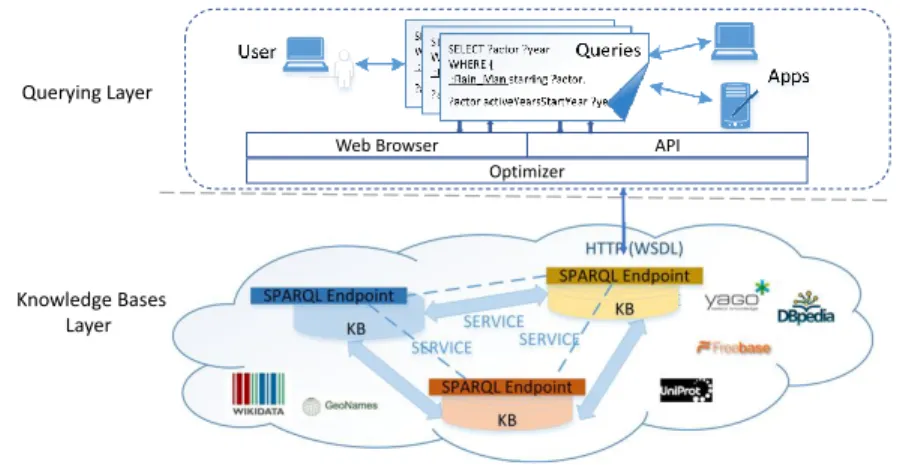
Figure1illustrates a generic architecture for querying curated KBs. In the knowledge bases layer (bottom), curated KBs (e.g., DBpedia2) usually use Resource Description Framework (RDF) as the data representation model because RDF has been accepted as the standard model by W3C3. RDF encodes a relationship (or fact) with a tri-ary tuple (i.e., triple): (subject,predicate,object), (s,p,o) for short. Moreover, RDF allows the sharing and reuse of data across boundaries [10]. In order to allow users perform querying over knowledge bases, a service is built upon each knowledge base. The service is called SPARQL (SPARQL Protocol and RDF Query Language) Endpoint and is realised by the HT TP bindings provided by KBs. SPARQL includes two parts: a standard query language for RDF and the protocol, which uses Web Services Description Language (WSDL) to describe a means for conveying SPARQL queries to an SPARQL query processing service and returning the query results. SPARQL Endpoint also realises the potential of federated SPARQL through SERVICE keyword introduced in SPARQL 1.1 specification, whereby several SPARQL Endpoints are combined allowing complex queries to be run across a number of KBs. To the clients (i.e., query issuers), a SPARQL Endpoint acts as a machine-friendly interface towards each knowledge base.

Web Browser API

Optimizer Querying Layer

Knowledge Bases Layer

Fig. 1. Querying Curated Knowledge Bases

1 https://en.wikipedia.org/wiki/Main_Page 2 http://wiki.dbpedia.org/ 3 https://www.w3.org/

In the querying layer (top), a natural language question is transformed into a structured query which is executed against a KB and the answers are returned. Currently, querying SPARQL End-points has the problems like network instability and latency, which affect the query efficiency. Dumping the data and setting up local SPRAQL Endpoint is a solution, but data in a local Endpoint is not up-to-date and hosting an Endpoint requires expensive infrastructural support. Many re-search efforts have been dedicated to circumvent this problem [16,17,25–27] and caching is one of the popular directions [23]. While most research efforts focus on providing a server-side caching mechanism, being embedded in triple stores, client-side caching has not been fully explored [17]. Server-side caching is usually embedded in the background databases. Sometimes they are part of the query optimizer. Server-side cache is well developed but it is not customized to catch the different querying patterns from clients. Moreover, the design and development of server-side cache highly depend on the knowledge of background databases/servers. Therefore, it is not easy to develop a generic approach. On the other hand, client-side caching is a technique from Web applications, where the background databases/servers are black boxes to the Web users. Using client-side caching avoids making repeated requests to the servers and can quickly get answers. In addition, it is possible to collect client’s querying behaviours. In this article, clients refer to the users who perform the querying on SPARQL Endpoints. A user can be a human or a machine.

Our approach, SPARQL Endpoint Caching Framework (SECF), adopts the client-side caching idea and is domain-independent. In other words, our approach does not require the knowledge on what kind of data and how they stored in the knowledge base. SECF caches the (query, result) pairs for current processing query and its similar queries. This is motivated by the observation that end users who consume RDF-modelled knowledge typically use programmatic query clients, e.g., software or services to retrieve information from SPARQL Endpoints [16]. These queries usually have repetitive query patterns and only differ in specific elements of a triple pattern (a triple pattern is similar to a triple, except that at least one element namely subject, predicate or object, is a variable). Moreover, they are usually issued subsequently. To illustrate, Figure2gives two example queries that are structurally similar. Query 1 retrieves start year (i.e., the year their acting careers started) from the actors of the movieRain Manand the year should be later than 1980. Query 2 requests similar information but for a different movie (Eyes Wide Shut). The differences between these two queries are the movie names (the underlined terms) and the year in the Filter expression. By considering these observations, we propose to prefetch and cache the query results of similar queries in advance. Since the subsequent queries have high possibility to be the similar queries that are cached, the results will be returned immediately (if cached) rather than being retrieved from SPARQL Endpoints. Therefore, the average query response time will be reduced.

The problem then turns into how to find similar queries that are potential subsequent queries. To this end, SECF utilizes machine learning techniques to learn from the historical queries and captures

Query 1

SELECT ?actor ?year WHERE {

:Rain_Man dbpedia-owl:starring ?actor . ?actor dbpedia-owl:activeYearsStartYear ?year . }

FILTER(?year>1980) Query 2:

SELECT ?actor ?year WHERE {

:Eyes_Wide_Shut dbpedia-owl:starring ?actor . ?actor dbpedia-owl:activeYearsStartYear ?year . }

FILTER(?year > 1960)

the querying characteristics of the users. The key challenge centres on how to transform queries into vector representation that can be used by learning algorithms. We proposeTemplate-based feature modellingto transform a SPARQL query into a vector using the distances between this query and a set of “template queries". Each distance is considered as a feature value in this vector. This modelling approach drastically reduces the computation time compared to the state-of-the-art clustering-based feature modelling presented in [7]. SECF then modifies thek-Nearest Neighbour (k-NN) [1] model to learn from the feature vectors of training queries and to suggest similar queries of a new issued queryQ. The suggestion process runs in the background thread. The training set will be updated periodically to reflect the changes. Thus, the training process will accordingly perform in a periodical manner. After identifying similar queries, SECF prefetches the results of these similar queries and caches the (query, result) pairs.

As the cache space is limited, less useful data should be removed from the cache. A cache replacement algorithm is introduced for this purpose. However, techniques for relational databases are page-based (e.g., LRU-k [20]), which cannot be directly applied into our client-side caching framework because our caching is record based. Moreover, our client-side application is not based on relational database management system (RDBMS). In this article, we use atime-aware frequency based algorithm, which leverages the idea of a novel approach recently proposed for caching in main memory databases inOnline Transaction Processing (OLTP)systems [15]. More specifically, we propose and develop Modified Simple Exponential Smoothing (MSES) to evaluate the hit frequencies of cached queries and remove the ones with the lowest frequencies from the cache.

The contributions of this work are three folds. Firstly, we address the problem of providing a learning-based approach for accelerating query answering process for SPARQL Endpoints and design a caching framework. The framework can be deployed as a Web browser plugin, but ultimately we envisage it being embedded within SPARQL Endpoints that act as clients to other SPARQL Endpoints. Secondly, SECF suggests similar queries by leveraging machine learning techniques. The distance measurement for SPARQL queries considers both Basic Graph Patterns (BGPs) and the most used SPARQL operators. SECF also provides a time-aware smoothing-based cache replacement algorithm. Thirdly, we perform extensive experiments on real world queries to showcase the effectiveness of SECF.

The remainder of this paper is structured as follows. We give some background knowledge and overview the related work in Section2. Then we introduce SECF and the technical details in Section 3. The experimental results are reported in Section4. We give some discussions in Section5and finally conclude this article in Section6.

2 BACKGROUND

In this section, we briefly introduce the SPARQL query language and then we overview the related work.

2.1 SPARQL Preliminary

The official syntax of SPARQL1.1 considers operators OPTIONAL, UNION, FILTER, SELECT and concatenation via a dot symbol (.) to group patterns. VALUES and BIND are to define sets of variable bindings. We useB,I,L,V for denoting the (infinite) sets of blank nodes, IRIs, literals, and variables. A SPARQL graph pattern expression is defined recursively as follows [22]:

(i) A valid triple patternT ∈ (IV B) × (IV) × (IV LB)is a graph pattern,

(ii) IfP₁andP₂are graph patterns, then expressions (P₁ANDP₂), (P₁UNIONP₂) and (P₁ OP-TIONALP2) are graph patterns,

(iii) IfP is a graph pattern andRis a SPARQL built-in condition, then the expression (P FILTER

R) is a graph pattern.

ABGPis a graph pattern represented by the conjunction of multiple triple patterns. A SPARQL query can be decomposed into BGPs for certain operators and the result that can be regarded as a hierarchical tree. The decomposition is defined as follows:

Definition 2.1. (SPARQL Query Decomposition) LetQ=(S_Q,P_Q)be the query whereS_Qis the SELECT expression andPQ =P1⊕...⊕Pnis the query pattern with⊕ ∈{AND, UNION, OPTIONAL,

FILTER, BIND, VALUES, MINUS}. When pattern feature⊕ ∈{AND, UNION, OPTIONAL, MINUS}, graph patternPi,i∈ [1,n]can be recursively decomposed to sub-level graph patterns until the graph pattern is a BGP which can be further decomposed to triple patterns asPbдp,i =T1⊕...⊕Tk, where

⊕=AND. When pattern feature⊕ ∈{FILTER, BIND, VALUES}, graph patternPi cannot be decomposed to BGPs and is represented as expressions.

2.2 Related Work

Our work mainly addresses caching problems in two research areas, namelyQuery Cachingand Query Suggestion. We review the recent representative works of these two areas in this section.

Query cachinghas the rationale that it keeps the historical data for the usage of new queries. If new queries use the same data, results can be returned immediately, reducing the overall query response time. Query caching was originally developed in database communities and in recent years, has been extended to triple stores that manage SPARQL queries. Martin et al. [17] first proposed caching for SPARQL queries, in which both the complete triple query result and the application object are cached. However, this approach only considers repeated identical queries, while our work takes both identical and similar queries into consideration. The latter ones have high potential to be requested. Yang and Wu [27] developed an approach that caches intermediate result of basic graph patterns in SPARQL queries. For a new query, the approach checks if the result of any BGP or join of BGPs of this query is cached. The hit results are joined with the other parts of the query to form the final query result. This approach is designed to be embedded in a triple store and works with the query processing mechanism in the triple store. Very recently, Papailiou et al. [21] introduced canonical labelling to identify isomorphic subgraphs in SPARQL query patterns, which are cached for subsequent querying. This solution implements a caching layer on top of the distributed partitions and dynamically updates the contents of the cache. Verborgh et al. [26] proposed a Linked Data Fragments (LDF) approach, aiming at improving data availability. It can also be regarded as a caching technique because it caches fragments of queryable data from servers that can be accessed by clients. Each client is able to process SPARQL queries on replicated fragments cached from servers.

Query suggestionis usually adopted in search engines to better understand users’ information needs with the ultimate goal to improve the recall of querying. Researchers recently introduce query suggestion to improve the SPARQL querying. Lehmann et al. [14] proposed to leverage a supervised learning framework to suggest SPARQL queries based on examples previously selected by users. This approach narrows the range of possible answers asked by users and requires no knowledge of the underlying schema or the SPARQL query language. Hasan [7] used a suggestion model to predict the performance of newly issued SPARQL queries. The model is trained with previously issued queries and corresponding query performance, e.g., query time. For new queries, their performances can then be predicted from the trained model. The key contribution is that the SPARQL queries are modelled as feature vectors. However, their feature modelling method is very time-consuming. Query relaxation is closely related to query suggestion and extends the original

query to obtain more information by removing some constraints (e.g., “ages of the students in a class" returns more data than “ages of the female students in a class" by removing the constraint “female"). In recent years, query expansion techniques have been used by several research efforts on SPARQL queries. Elbassuoni et al. [2] proposed multiple types of relaxation methods to improve the recall of entity-relationship search. Lorey et al. [16] clustered similar SPARQL queries to different templates in order to detect recurring patterns in queries. These templates can be used to expand queries for query processing. Fokou et al. [4] investigated query relaxation over RDF data and focused on identifying parts of SPARQL query that are responsible for the failure of the query. A recent work proposed by Zhang et al. [29] expands a query in order to obtain accessed triples when executing the query. Caching these accessed triples will help facilitating subsequent queries that might need to access them. The work expands a queryQaccording to the triple patterns ofQ. A new query is generated by picking and modifying one of the triple patterns ofQand keeping the other parts inQ.

3 THE SPARQL ENDPOINT CACHING FRAMEWORK 3.1 Overview

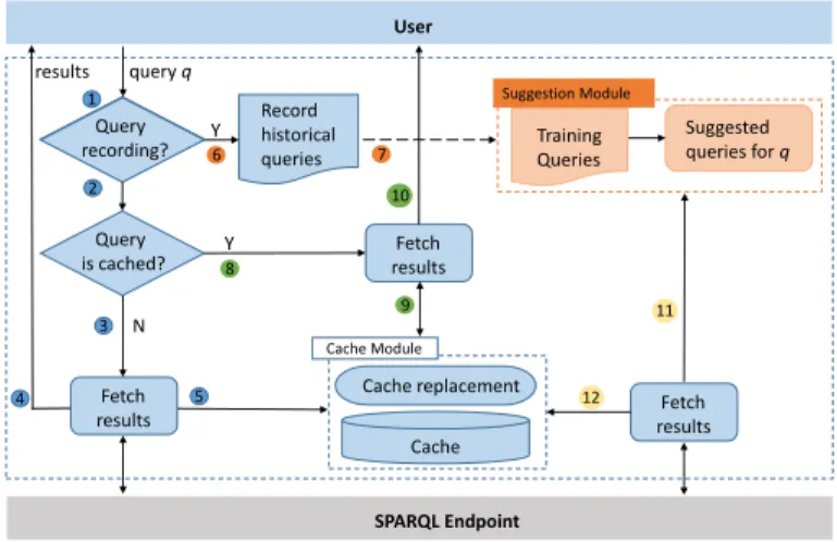
Figure3illustrates the working processes of SECF. We use different color of numbering to depict the different processes in this framework. The blue numbers are about fetching query results directly from SPARQL Endpoint. The green ones show the process that the results are returned from the cache. The orange numbers are for the suggestion process while the yellow numbers are for caching suggested queries into the cache. When a new query is issued, SECF first checks if query recording is enabled (○1). If yes, a background process will log all queries (○6). The logged queries are used for the suggestion process, including training and suggestion (○7). Then it checks if an identical query (either cached as an issued query or a suggested query) has been cached (○2). If not, SECF fetches (○3) and returns (○3) the results directly from the SPARQL Endpoint. These results are cached in the cache module (○5). If the results are in the cache (○8), they are returned immediately via the cache model (○9 and○10). When query suggestion is enabled, during run-time, suggested queries are generated for the current query in the suggestion module. The results of these suggested queries will be retrieved (○11) from the SPARQL Endpoint in advance and cached (○12), together with the queries in the form of (query, result) pairs(q_i,r_i). The aim of prefetching and caching similar queries in advance is to enhance the hit rate of cache (i.e., how much percentage

Query recording? Query is cached? Fetch results Record historical queries Query recording? Fetch results Cache replacement Cache Fetch results Training Queries Suggested queries for q Cache Module User SPARQL Endpoint results query q Suggestion Module 1 2 3 4 Y Y N 6 8 7 9 10 5 11 12

of queries can be answered immediately from cached results). A cache replacement algorithm is executed when the cache is full or the number of cache queries is reached. It runs in a separate thread so that it does not affect the query answering process.

The overall query speed depends on the hit rate of the cache. As it is observed that most subsequent queries are similar to previous issued queries in [16], the prefetch/cache process will increase the number of queries that are hit. If we cache the similar queries, which are potential subsequent queries, higher hit rate can be achieved. To identify and cache similar queries, we propose a learning based approach that consists of following three main steps:

• Step 1:Feature modelling. We propose to model SPARQL query to feature vectors that can be fed into multiple learning algorithms. However, transforming a SPARQL query into vector representation is a challenging problem. We first introduce the distance measurement between SPARQL queries in Section3.2and then discuss our feature modelling approach based on this distance in Section3.3.

• Step 2:Training and suggestion. After obtaining the feature vectors of SPARQL queries, we train a suggestion model using historical queries as the training set. A trained model is the output. When a new queryQarrives, we first transformQto a feature vector using techniques from Step 1. Then we feed the vector into the trained suggestion model for similar queries recommendation. We introduce our approach in Section3.4.

• Step 3:Cache and replacement. We prefetch the results of similar queries. As the cache is with limited size, less useful queries (and their results) should be removed from the cache. We introduce our cache and replacement algorithm in Section3.5.

3.2 Query Distance Calculation

To find similar queries, we compute the distance between two given SPARQL queries by calculating the distance between patterns of the two queries:

d(PQ,P ′ Q)=d(Pbдp,P ′ bдp)+d(Pf ilter,P ′ f ilter)+d(Pbind,P ′ bind)+d(Pvalue,P ′ value) (1)

WhereP_QcontainsP_bдp,P_{f ilter},P_bind,P_valueandP

′ QcontainsP ′ bдp,P ′ f ilter,P ′ bind,P ′ value.d(P_Q,P ′ Q)=

0 denotes the two queries are structurally the same.

3.2.1 BGP Distance.We propose to use Graph Edit Distance (GED) [24] to measure the distance

between BGPs because a BGP can be represented as a graph. In the graph,subjectandobjectare nodes linked bypredicateas the edge. GED between two graphs is the minimum amount of edit operations (i.e., deletion, insertion and substitutions of nodes and edges) needed to transform one graph to the other. However, different BGPs share the same graph, which contains two nodes and

(s, p, o) (s, ?p, o) (?s, p, o) (s, p, ?o)

(?s, ?p, o) (?s, p, ?o) (s, ?p, ?o) (?s, ?p, ?o)

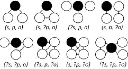
Fig. 4. Mapping Triple Patterns to Graphs. Eight types of triple patterns are mapped to eight structurally different graphs. Black nodes are conjunction nodes for clarity.sis forsubject,pis forpredicate,ois forobject. The question mark indicates that the corresponding component is a variable.

(s, p, ?o) (?s, p, ?o) group

(s, p, ?o) (?s, p, ?o)

:Rain_Man dbpedia-owl:starring ?actor . ?actor dbpedia-owl:activeYearsStartYear ?year

Fig. 5. Graph Modelling for BGPs in Query 1.

one edge. Therefore, the distance between each pair of BGPs is zero. In order to distinguish each BGP graph, we formulate the problem of modelling BGPs to distinct graphs as follows:

Problem 3.1. (BGP Graph Modelling) GivenP_bдp

i ={tp1,tp2, ...,tpn}denote a BGP of a SPARQL

query,tpk,k∈ (1,n)is a triple pattern rooted atP_bдp

i.дed(дo,дd)represents the graph edit distance

between graphдo and graphдd. BGP graph modelling is the task that models eachtpkto a graphдtpk

satisfyingдed(дtpk,дtpl)>0whenk,l.

To address the above problem, we propose to map all the eight types of triple patterns to eight structurally different graphs, as shown in Figure4. The black circles denote conjunction nodes for clarity. They are not coloured in graph modelling. As we only consider the structures of queries, whether the connecting node represents a join or union is not distinguished. Therefore, the different meanings of connecting nodes are not considered in this work. Using these mappings, we model the triple patterns of BGPs in Query 1 in Figure2, to a graph, which is depicted in Figure5.

There are various ways to map triple patterns to graphs. However, in our work, the way that we choose for the mapping does not affect the final cache result very much. So we only focus on mapping distinct triple patterns to distinct graphs. The reason is that in our work, similar queries that can lead to a cache hit are mostly the ones that are structurally the same with the current processing query. Specifically, thek-NN model first returns the structurally the same queries as similar queries, then returns the ones that are structurally the same but with different filter and bindings, and finally returns structurally similar queries. As the queries are mostly issued by programmatic clients and are generated with query templates (as described in Section1), most returned queries are the ones using the same template, i.e., are structurally the same. Thus the structurally similar queries will not affect the caching results much as they are with small numbers. So the distances between different triple patterns that are considered in measuring structurally similar queries give limited impact on caching performance. Therefore, the difference of various mapping ways is not considered here.

3.2.2 Other Distances.We calculated(P_{f ilter},P

′

f ilter),d(P_bind,P

′

bind)andd(P_value,P

′

value)only whend(P_bдp,P

′

bдp) = 0. We define distance between two FILTER expressions as half of their levenshteindistance when the variables in these two expressions are identical, otherwise the distance is a fixed value 1. Thus the distance is in the range of[0,0.5]or equals to 1.

d(P_{f ilter,i},P_{f ilter}′ _,i)=

( _{levenshtein(E(i),E}′

(i))

2max(lenдth(E(i)),lenдth(E′(i))), i f V(i)=V

′ (i) 1, else (2) whereE(i)andE ′

(i)represent the FILTER expression forP_{f ilter,i}andP

′

f ilter,i.V(i)andV

′

(i)are variables in these two FILTER patterns respectively. When there are multiple Filter expressions

that can be compared, the total difference is defined as: d(Pf ilter,P ′ f ilter)= m Õ i=1 d(Pf ilter,i,P ′ f ilter,i) (3)

Filter expressions in Query 1 and Query 2 are similar as the distance is 0.05 using Equation (3). So

d(P_Q1,P

′

Q2)=0.05 (Equation (1)). We also have similar functions for BIND and VALUE patterns.

3.3 Feature Modelling

Using the distance function Equation (1), it is intuitive to suggest similar queries to a given query

Q by calculating the distances betweenQand each historical query, then rank the distances in descending order and find the topksimilar ones. However, the calculation of distances between

Q and each historical query is time-consuming when the number of historical queries is large. Moreover, it cannot leverage the machine learning algorithms to facilitate the suggestion process because machine learning algorithms require the vector representation of objects [6]. Therefore, we choose to construct feature vectors for SPARQL queries that leverages the distances and can facilitate the similar queries suggestion. It is worth mentioning that the work in [7] proposes an approach to transform SPARQL query to vector representation. For comparison, we firstly introduce the approach in [7], which we refer to ascluster-based feature modelling(Section3.3.1) and then discuss our approach, thetemplate-based feature modelling(Section3.3.2).

3.3.1 Cluster-based feature modelling.In cluster-based feature modelling, distances between

each pair of queries in the training set are calculated using only BGP distance. Thenk-medoids algorithm [11] is utilized to cluster the training queries by using distance scores that are calculated. The center queries of each cluster are selected and the distance scores between each center query and a queryQis obtained to form a feature vector ofQ, where each score is regarded as an attribute of the feature ofQ. Thus the number of clusters equals to the number of dimensions (i.e., the number of feature attributes) of the feature vector ofQ.

3.3.2 Template-based feature modelling.The cluster-based feature modelling requires distance

calculation between all training queries. Moreover, the clustering process adds additional time consumption. To reduce the feature modelling time, we propose to replace the center queries used in cluster-based feature modelling with representative queries that are generated by benchmark templates. Specifically, we generate queries from 18 out of 25 valid templates in the DBPSB bench-mark [18] (we excluded queries which do not return any results: Query 1, 2, 3, 10, 16, 21 and 23). We refer to these queries astemplate queries. By recording the distance scores between a queryQ with the 18 template queries, we obtain an 18-dimension feature vector forQ. The computation is then drastically reduced fromO(n2)in cluster-based feature modelling toO(n), wherenis the number of queries. Therefore, our approach is feasible to apply to large size of training sets.

Moreover, we adopt three dimension reduction algorithms, namely Canonical Correlation Anal-ysis (CCA) [8], Principal Component Analysis (PCA) [9] and Non-negative Matrix Factorization (NMF) [13] on the feature vectors. In machine learning, dimension reduction is the process of reducing the number of random variables to describe a large set of data while still describing the data with sufficient accuracy. It helps reducing the learning time on the feature vectors. CCA calculates the coefficient among all features and chooses the most uncorrelated features. PCA aims to find a linear transformation to project the original data to a lower-dimensional space which is as informative as possible to capture as much of the variance of the original data in an unsupervised manner. NMF finds approximate decomposition of original data matrix and thus reduces the dimension by storing the two decomposed lower dimensional matrices.

Training Queries q ... C1 C2 Cn d1 d2 ... dn d1 d2 dn D1 D2 ... D(n-1)n/2

dI : Distance between q and center query of Ci

Ci : Cluster

Dj : Distance between training queries

(a) Cluster-based q d’1 d’2 ... d’18 d’1 t1 t2 t18 d’2 d’18 DR (CCA PCA NMF) f’1 f’2 ... f’r ti : Template query

d’i : Distance between q and ti

f’j : Feature after dimensional reduction on d’1 to d’18

(b) Template-based

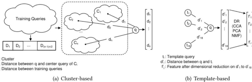
Fig. 6. Feature Modelling. The cluster-based modelling (a) is based on the distances among each pair of all the training queries. Clustering is done using these distances.di is the distance between queryQand the center query of the clusterCi, and it represents a feature ofQ. The template-based modelling (b) uses template queries. The distance betweenQand template queryti represents a feature ofQ. After dimensional reduction (DR), the features are extracted tof1′tof

′

r wherer<18.

Figure6illustrates the process and difference of cluster-based feature modelling and template-based feature modelling. In Figure6(a), the modelling is based on all training queries.{D(n−

1)n/2

i=1 }

record distances between each training queries.{C_in

=1}denote clusters.{d

n

i=1}are distances between

queryQand center queries of clusters. In Figure6(b),t1tot18are template queries.d1

′

tod18

′

are distances between queryQand 18 template queries.f1

′

to f_r′are features that are obtained after applying dimensional reduction algorithm (i.e., CCA, PCA or NMF), wherer <18.

3.4 Suggesting and Prefetching Similar Queries

After the feature vectors are obtained (Step 1 in Section3.1), we train a suggestion model with the feature vectors of training queries and suggest similar queries to a new query (Step 2). We adopt

k-Nearest Neighbours (k-NN) [1] as prediction model becuase it is one of the two common types of similarity searches [12].k-NN is a non-parametric classification and regression algorithm that predicts the performance of new data point based on itsk-nearest training data points:

pnew = 1 k k Õ i=1 (p_i), (4)

wherep_new is the predicted value of the new data andp_i is the performance of thei-th nearest training data. If the new data is not in the training set,k-NN finds the point which is the closest to the new point according to its features.

k-NN is often successful in the cases where the decision boundary is irregular, which applies to SPARQL queries [7]. It is originally a supervised learning algorithm which requires labels (or classes). Ak-d tree is built for the training data (points) with labels. For a new point, itsknearest neighbours in the tree are searched and its label (or class) is decided by the labels of these neighbours. In our work, we do not have labels and the task is not to classify the data points (a point refers to a query in this work) but to find the data points that are close to a given point. We therefore modify

k-NN algorithm to only build thek-d tree according to the Euclidean distance between feature vectors of SPARQL queries and we omit the label part. Thek-NN thus turns into an unsupervised learning algorithm. Then we use trainedk-NN model to suggest the nearest (i.e., the most similar) queries for a new query. Given the similar queries for a queryQ, we prefetch the results of these queries directly from SPARQL Endpoints and put the(q_i,r_i)pairs into the cache during the caching process.

3.5 Caching and Replacement

As the cache has limit space, the less useful data should be removed from the cache to give space to more useful data. In traditional page-based cache in databases, the less useful data is less frequently accessed which will be removed to give space to more frequently accessed data. When the data required by a new query is in the cache, the result is returned immediately. Each time the data in cache is accessed, it is called acache hit. Therefore, the problem of cache replacement is the problem of identifying the more frequently accessed data.

SECF, the proposed client-side caching framework, does not require the knowledge of underlying system of SPARQL Endpoint. Thus we cannot directly apply the cache replacement algorithms used in page-based databases. We propose to use atime-aware frequencybased algorithm, which leverages the idea of a novel approach recently proposed for caching in main memory databases in Online Transaction Processing (OLTP)systems [15]. Specifically, we cache the (query, result) pairs and consider the hit frequencies of them when performing cache replacement. The recently most hit queries in the cache arehotqueries which are more useful queries. Hot queries will be kept in the cache, whereas queries in the cache that do not belong to hot queries are considered less useful, which will be removed from the cache.

Before we introduce the proposed cache replacement algorithm, we introduce how to measure the hit frequencies of queries in Section3.5.1. Then we apply the proposed frequency measurement in developing two cache replacement strategies in Section3.5.2.

3.5.1 Modified Simple Exponential Smoothing (MSES).We adapt the algorithm used for

identify-ing hot triples in our previous work [29]. Here we introduce this algorithm and how we adapt it to identify hot queries.

TheExponential Smoothing(ES) is a technique to produce a smoothed data presentation, or to make forecasts for time series data, i.e., a sequence of observations [5]. It can be applied to any discrete set of repeated measurement and is currently widely used in smoothing or forecasting economic data in the financial markets. Equation (5) shows the simplest form of exponential smoothing. This equation is also regarded asSimple Exponential Smoothing(SES).

Xt =α∗xt+(1−α) ∗X_t−1, (5)

whereX_tstands for smoothed observation of timet,x_tis the actual observation value at timet, and

αis a smoothing constant withα∈ (0,1). From this equation, it is easy to observe that SES assigns exponentially decreasing weights as the observation becomes older, which meets the requirement of selecting the most frequently and recently issued queries. The reason behind our choice of SES is its simplicity and effectiveness [15].

In SECF, we exploit SES to estimate hit frequencies of queries. In this case,x_trepresents whether the query is hit at timet, thus it is either 1 for a cache hit; or 0 otherwise. Therefore, we can modify Equation (5) toModified Simple Exponential Smoothing(MSES):

Et =α+Etpr ev ∗ (1−α)tpr ev

−t

(6) wheret_{pr ev}represents the time when the query is last hit andE_t

pr ev denotes the previous frequency

estimation for the query att_{pr ev}.E_tdenotes the new frequency estimation for the query att[15]. The accuracy of MSES can be measured by its standard error. We gave the derivation and the standard error of Equation (6) and provided a theoretical proof that MSES achieves better hit rates than the most used cache replacement algorithm LRU-2 in [29].

3.5.2 Cache Replacement Algorithms.We perform cache replacement based on the estimation

score calculated by MSES. Each time a new query is executed, we examine the frequency of cache hit of this query using MSES. If it is in the cache, we update the estimation of frequency for it.

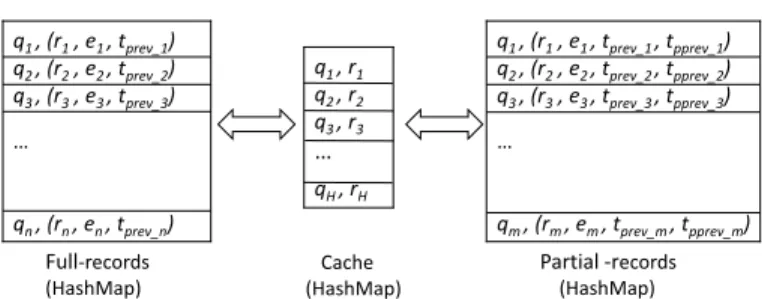
q₁ , r₁ q2 , r2 q₃ , r₃ … qH, rH q₁ , (r₁, e₁ , t_{prev_1}) q2 , (r2, e2 , tprev_2) q₃ , (r₃, e₃ , t_{prev_3}) … q_n, (r_n, e_n, t_{prev_n}) Cache (HashMap) Full-records (HashMap) q₁ , (r₁, e₁ , t_{prev_1} , t_{pprev_1}) q2 , (r2, e2 , tprev_2 , tpprev_2) q₃ , (r₃, e₃ , t_{prev_3} , t_{pprev_3}) … q_m, (r_m, e_m, t_{prev_m}, t_{pprev_m}) Partial -records (HashMap)

Fig. 7. Cache and Two Types of Records for Two Replacement Strategies.qidenotes a query;ri denotes the results ofqi;eiis the estimation of records calculated by Equation6;tpr ev_iis the last timeqi was hit in the

cache;tppr ev_iis the second last timeqiwas hit in the cache;His the number of hot queries can be cached;n is the total number of historical queries;mis the number of historical queries recorded in the partial records. Otherwise, we just record the new estimation. In order to realise the replacement, we use one hash map to store contents in the cache and the other hash map for recording information of historical queries. Figure7depicts the two hash maps. Cache stores the query and its results, denoted as (q_i,r_i), whereq_i is the key andr_i is the value. In the full-records,q_i is the key andr_i,e_i,t_{pr ev}_iis

the value. In the partial records, one more information, the second last hit time ofq_i is recorded and it is denoted ast_{ppr ev}_i. When the cache is not full,(qi,ri)are cached. Accordingly, related

information is stored in the records. When the cache is full, replacement is required.

To decide which records can be kept in the cache, we develop two cache replacement strategies, namely theFull-records replacementand theImproved replacement. The difference of these two strategies is whether to keep the full records of the historical queries or not.

Full-records replacement.In the full-records replacement, the algorithm keeps the estimation records for all processed queries. Specifically, it processes all the historical queries. When en-countering a hit to a query at timet, the algorithm updates this query’s hit frequency estimation using Equation (6). When the scan on records is completed, the algorithm ranks each query by its estimated frequency and returns theH queries with the highest estimates as the hot set. These top-Hqueries are kept in the cache, while lower ranked queries will be removed from the cache. However, this algorithm requires storing the whole estimation records which produces large over-head. Furthermore, it consumes a significant amount of time when calculating and comparing the estimation values. To solve these issues, we consider improving the algorithm in two ways. One possible solution is that we just keep a record after skipping certain ones. This is a naive sampling approach. We vary the sampling rate but it turns out that the performance of this sampling approach is not desirable (see Section4.3). The other possible approach is that we maintain partial records by only keeping those within a specified range of time.

Improved replacement.In the improved replacement, we only keep estimation records from a certain point of time to the current time to reduce the space overhead of the records. If we only keep very short records, the new cached query may fail to find its last estimation. In that case, the new estimated frequency of this query may be very small and it will be incorrectly removed from the cache. If we keep very long records, the space overhead is an issue as we discussed in full-records cache replacement. So we propose a solution that additionally keeps the second last hit time of a query in the records. Then we measure the maximum time gap between the last hit time and the second last hit time for each query in the records. After that, we use current time to minus this maximum time gap and get a previous time, which is the time that we start to keep the records. All the records before this time will be deleted.

Table 1. Selected patterns from SELECT queries. FILTER occupies large proportion in SELECT queries FILTER VALUE BIND

DBpedia3.9 83.97% 0.81% 0.06% LinkedGeoData 50.72% 0.005% 0.0006%

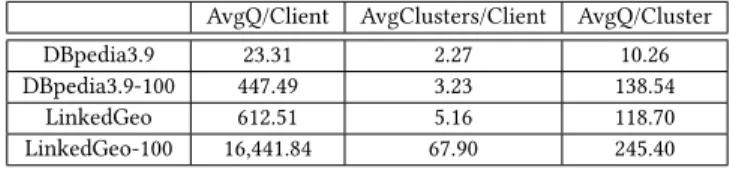
Table 2. Analysis of clients associated with queries and clusters AvgQ/Client AvgClusters/Client AvgQ/Cluster

DBpedia3.9 23.31 2.27 10.26

DBpedia3.9-100 447.49 3.23 138.54

LinkedGeo 612.51 5.16 118.70

LinkedGeo-100 16,441.84 67.90 245.40

4 EVALUATION

We evaluate our proposed framework in this section. We first describe the setup of our evaluation environment (Section4.1). Then we provide a detailed analysis of the real-world queries used in the evaluation (Section4.2). Finally, we report the experimental results, including the performance comparison of cache replacement algorithms, feature modelling approaches and the performance comparison to the state-of-the-art work (Section4.3to4.5).

4.1 Setup

Datasets.We analysed the query logs from DBPedia’s SPARQL Endpoint4 (DBpedia3.9) and Linked Geo Data’s Endpoint5(LinkedGeoData) provided by USEWOD 2014 challenge. We extract queries by decoding, identifying SPARQL queries from query strings and removing incomplete queries and queries with syntax errors according to SPARQL1.1 specification. We focused on SELECT queries in the experiments and retrieved 198,235 valid queries from DBpedia3.9 and 1,790,047 valid queries from LinkedGeoData. Among these queries, 83.97% DBpedia3.9 queries and 50.72% LinkedGeoData queries have FILTER operator (Table1).

Implementation and System.We obtained BGPs by parsing the SPARQL queries using Apache Jena-2.11.2. We implemented GED using a suboptimal solution integrated in the Graph Matching Toolkit6. The modifiedk-NN and LRU-2 were implemented in Java. Specifically, we adopted Weka library7to build thek-d tree fork-NN. We set up our own SPARQL Endpoint by installing local Virtuoso server and loading datasets into the Virtuoso. The server has the configuration of 64-bit Ubuntu 14.4 with 16GB RAM and 2.40GHz Intel Xeon E5-2630L v2 CP U. Our code runs on a PC with 64-bit Windows 7, 8GB RAM and 2.40GHZ Intel i7-3630QM CP U.

4.2 Analysis of Real-world SPARQL Queries

4.2.1 Analysis of Average Queries. We used the distance measurement described in Section3.2

to cluster the queries. Table2shows that the average queries for a client in DBpedia3.9 log files is 23.31, and the average clusters a client’s queries belong to is 2.27. The average queries in each cluster is 10.26. For LinkedGeoData queries, the average queries per client is 612.51 and each client’s queries belong to 5.16 clusters in average. The average queries in each cluster is 118.70. Our analysis shows that each client performed several queries which have shared clusters, indicating clients issued similar queries.

4 http://dbpedia.org/sparql/ 5 http://linkedgeodata.org/sparql 6 http://www.fhnw.ch/wirtschaft/iwi/gmt 7 https://weka.wikispaces.com/

0 1000 2000 3000 4000 5000 6000 7000 8000 9000 0 2 4 6 8 10 12x 10 6 Unique Client ID A v e ra g e T im e G a p t o N e x t S im ila r Q u e ry ( s e c o n d s ) (a) DBPedia3.9 0 500 1000 1500 2000 2500 3000 0 0.5 1 1.5 2 2.5 3 3.5x 10 7 Unique Client ID A v e ra g e T im e G a p t o N e x t S im ila r Q u e ry ( s e c o n d s ) (b) LinkedGeoData

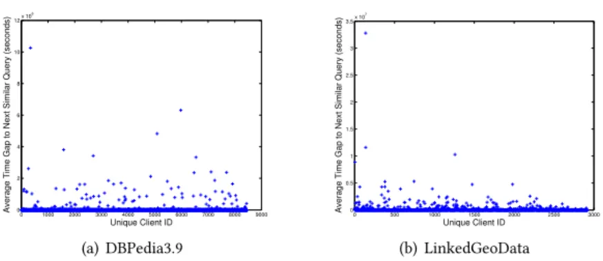
Fig. 8. Analysis of Average Matched Time. Similar queries are usually issued within a short period of time.

We also selected 100 clients with the most queries issued and found that the average number of queries for these top clients in DBpedia3.9 is 447.49 and the average clusters for one client is 3.23. The average queries per cluster increases to 118.70. The numbers for the top 100 clients who issued most queries in LinkedGeoData are higher, as average queries per client is 16,441.84, and average number of clusters per client is 67.90. In average, 245.40 queries belong to one cluster. These findings indicate that clients performed a large number of queries which have similar structures. The average number of queries for one cluster shows that queries have high similarity.

4.2.2 Analysis of Subsequent Queries.To estimate how likely it is that queries are similar to

previous queries and therefore could benefit from the prefetched results, we evaluated the time difference between one query and the next matched query (i.e., the next query belonging to the same cluster) for each client. DBpedia3.9 log files have a total of 8,500 distinct client IDs and LinkedGeoData has 2,921 distinct client IDs. We assigned distinct IDs starting from 1 for clients of both datasets. Figure8shows the average time gap between two matches for both datasets. Blue crosses indicate the average time gap (to next matched query) for each client ID. From Figure8(a), we can see most of the time gap are close to zero, positioning blue cross on the X-axis, which means that the client issues similar-structured queries subsequently. A small number of blue crosses are away from the X-axis, which means that these clients seldom issue similar-structured queries. Similar observations are found in Figure8(b). It demonstrates the fact that most clients issue similar queries subsequently. Moreover, on average, the similar queries are issued by the same client with previous queries within a very close time period. This further confirms that our approach can benefit the clients’ subsequent queries in terms of querying answering speed.

4.3 Performance of Cache Replacement Algorithm

We firstly evaluated our cache replacement algorithm MSES, because it would be used in the following experiments. To evaluate the performance of MSES, we implemented various algorithms including the full-record MSES, improved MSES, the sampling MSES, and LRU-2. LRU-2 is a commonly used page replacement algorithm which we implemented based on record rather than page. All of LinkedGeoData valid queries obtained were processed in this experiment because the size of this query set is much larger than DBpedia3.9 query set. Thus we can observe the difference between Improved MSES and MSES algorithms.

0 2 4 6 8 10 12 14 16 18 x 105 0 10 20 30 40 50 60 70 Queries Processed H it R a te ( % ) 0.05 0.7 0.03 0.01

(a) Different alpha

0 2 4 6 8 10 12 14 16 18 x 105 0 10 20 30 40 50 60 70 Queries Processed H it R a te ( % ) MSES Sampling MSES Improved MSES LRU−2

(b) Different cache replacement

10 20 40 50 0 100 200 300 400 500 600 700 800 900

Percentage of Hot Queries (%)

M a x im u m R e c o rd s S iz e ( K B ) MSES Improved MSES Hot Size

(c) Space overhead of MSES

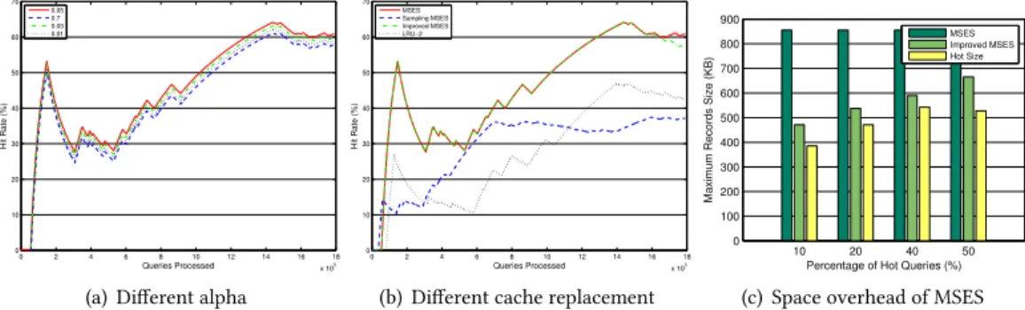
Fig. 9. Cache Replacement Performance (LinkedGeoData). Different values ofαhave different impact on the hit rates (a). Different cache replacement algorithms affect the hit rates largely (b). The improved MSES reduces the space overhead largely compared to the MSES (c).

Impact ofα.As theExponential Smoothinghas only one parameterα, the choice forαwould affect the hit rate performance. However, as per our experiments on different values forα, the hit rates differ only slightly and a value of 0.05 shows better performance, as shown in Figure9(a).

Impact of Cache Replacement Algorithms.Figure9(b)shows the hit rates achieved by the four algorithms we implemented. It should be noted that in the experiment, the caching size was set to 20% of the total historical queries andαwas set to 0.05 for MSES and its variants. We chose 20% as the caching size because it is neither too large (e.g.,>50%) to narrow the performance differences among algorithms, nor too small (e.g.,<10%) leading to inaccurate performance evaluation due to insufficient processed data. From the figure, we can see that MSES and Improved MSES have the same hit rate until they have processed about 1.5 million RDF triples, after which MSES has a higher hit rate than Improved MSES. This is because MSES maintains the estimations for all processed records while the Improved MSES only keeps part of the estimations. The changing point denotes that from which, the Improved MSES maintains partial volume of estimation records. From the figure, we can also see that Sampling MSES does not perform well. This figure only shows the hit rate of sampling MSES with the sampling rate of 50%, which is expected to have a high hit rate. The LRU-2 algorithm has the lowest hit rate of all the algorithms. The hit rates of all algorithms start from 0 and reach their first peak at certain points, then fluctuate. The direction to the first peak shows the warm-up stage and the rest of the lines are the warmed stage. This illustrates that we exploit an incremental approach, which includes a warm-up stage to calculate the hit rate.

Space Usage for Records.Figure9(c)gives the measurement of space usage by recording the estimations. As discussed before, MSES performs better than the Improved MSES. However, it consumes more storage space to maintain the estimation records for all processed triples. It also takes longer time to check the cache. Figure9(c)shows the maximum space consumption for each algorithm. Note that we used all valid LinkedGeoData queries in this experiment. The columns are classified into four groups which represent the percentage of hot queries to all processed queries. In each group, the left column represents the maximum space used by MSES, including the hot queries and the estimation records. The middle column represents the space usage of the Improved MSES that also includes the hot queries and the estimation records. The right column represents the size of the hot queries. From this figure, we can see that the Improved MSES consumes less space.

2 3 4 5 6 7 8 9 50 55 60 65 70 75 80 85 90 95 Dimension A v e ra g e D is ta n c e t o T e s t Q u e ry PCA CCA NMF

(a) Distances for C10 (DBpedia3.9)

Dimension 2 4 6 8 10 12 14 A v e ra g e D is ta n c e t o T e s t Q u e ry 40 45 50 55 60 65 70 75 80 PCA CCA NMF

(b) Distances for C15 (LinkedGeoData)

Fig. 10. Performance Comparison among Using CCA, PCA and NMF to Reduce Dimension (Cluster-based)

4.4 Comparison of Feature Modelling Approaches

In the experiments of this section, we compared our feature modelling approach (i.e., template-based feature modelling) with the state-of-the-art approach (i.e., cluster-template-based feature modelling), and evaluated the performance under the scenarios of applying and without applying sugges-tion/prefetching. We applied the dimensional reduction algorithms on both template-based feature modelling and cluster-based feature modelling methods.

Because the time consumption of cluster-based approach is tremendous, we did not use all valid queries as the training set. We randomly chose 21,600 training queries and 5,400 testing queries from the two query sets separately. The cache replacement algorithm used in all testing cases is Improved MSES andα =0.05. Because the larger size of cache, the higher hit rate it would achieve, we only show experimental results when the number of queries in cache is set to 1,000.

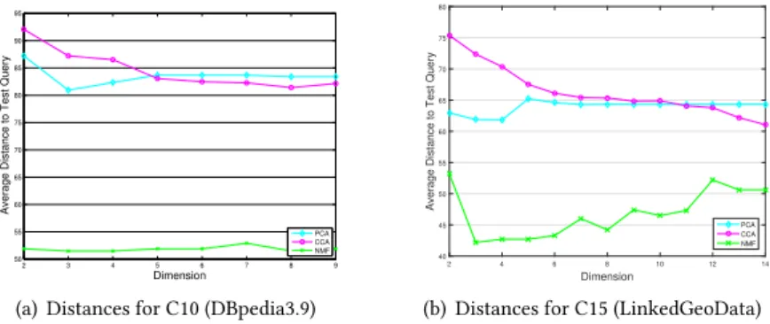
4.4.1 Performance of Cluster-Based Feature Modelling. In order to compare to template-based

feature modelling approach, we applied dimensional reduction algorithms on cluster-based feature modelling approach. We generated new feature files with different lower dimensions for DBpedia3.9 and LinkedGeoData queries using CCA, PCA and NMF discussed in Section3.3.2. The files are from Dimension 1 (D1) to D9 for DBpedia3.9 with 10 clusters (C10) and D1 to D14 for LinkedGeoData with 15 clusters (C15). We then trainedk-NN model with these files respectively and gotksuggested queries for a randomly chosen queryQ. We computed the average distance between suggested queries withQand computed the distances obtained when using CCA, PCA and NMF. The lower the average distance is, the better the suggestion is. As large amount of the queries from these two SPARQL Endpoints are similarly-structured or repeated (see Section4.2), we set a large number of queries to suggest to avoid the distance to be zero. Thus we chosek=500 ink-NN in this experiment. As shown in Figure10, NMF always performs the best for both DBpedia3.9 and LinkedGeoData queries. It gets optimal result when the number of dimensions is 3. PCA performs better than CCA when dimension is low and worse than CCA when dimension becomes high. For DBpedia3.9 queries, the intersection isD=5, while for LinkedGeoData, the intersection isD=11. We used NMF for our dimension reduction in the comparisons thereafter.

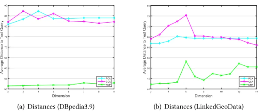
4.4.2 Performance of Template-Based Feature Modelling.In template-based feature modelling,

we also leveraged dimensional reduction algorithms. The performance of different algorithms is shown in Figure11. It is shown that NMF still outperforms other algorithms in extracting the most representative features.

Dimension 2 3 4 5 6 7 8 9 A v e ra g e D is ta n c e t o T e s t Q u e ry 50 55 60 65 70 75 80 85 90 PCA CCA NMF

(a) Distances (DBpedia3.9)

Dimension 2 4 6 8 10 12 14 A v e ra g e D is ta n c e t o T e s t Q u e ry 40 45 50 55 60 65 70 75 80 PCA CCA NMF (b) Distances (LinkedGeoData)

Fig. 11. Performance Comparison among Using CCA, PCA and NMF to Reduce Dimension (Template-based) Table 3. Time comparison on feature modelling approaches

Datasets Cluster-based modelling (sec.) Template-based Modelling (sec.)

Training Time

DBPedia3.9 33,446 1,109

LinkedGeoData 23,405 758

Average Query Time

DBPedia3.9 355 251

LinkedGeoData 234 158

Table3gives the impact of two feature modelling algorithms on time consumption. The training time is recorded for 21,600 training queries. Cluster-based approach requires 33,446 seconds, which is more than 9 hours for DBPedia3.9 queries, and 23,405 seconds (i.e., more than 6 hours) for LinkedGeoData queries. Template-based approach largely reduces the time to 1,109 seconds and 758 seconds, respectively. In terms of the average query time, our template-based approach also outperforms the cluster-based approach.

4.5 Performance Comparison with the State-Of-The-Art Work

We also compared our work with the Adaptive SPARQL Query Cache (ASQC) introduced in [17], as it is the first and complete work to cache SPARQL query in a client-side manner.

4.5.1 System Performance Comparison. In this experiment, we compared the average hit rate,

average query time and space usage between our work SECF and ASQC. We also gave performance when no cache was used. To compare our approach with ASQC, we modified the code of ASQC8to access our datasets. We performed the experiment on DBpedia3.9 dataset. We used Cluster-Based Feature Modelling and Improved MSES withα=0.05. Table4presents the results. The first three columns of Table4show the performance comparison. Compared to the hit rate of ASQC (72.63%), SECF (78.59%) increases the performance by 5.96%. ASQC takes 264 ms in average for one query and SECF takes 247 ms. So SECF reduces the query time by 6.44%. When no cache is applied, the average query time increases to 625 ms. We did not include prefetching time as it is in a separate thread. The improvements showcase the effectiveness of our learning based approach and provide a research direction for improving SPARQL query performance using machine learning techniques. Space consumption evaluates how much memory the cache uses. In SECF, the total usage (before slash) for caching 1,000 queries includes cached queries and answers as well as the estimation records for cache replacement (after slash). We used the same implementation for ASQC in order to compare. The results indicate that the most space is consumed by cached (query, result) pairs.

8

Table 4. Performance comparison

ASQC SECF No Cache

Hit 72.63% 78.59% NA AvgTime 264ms 247ms 625ms Space 7.15MB 7.15MB/0.45KB NA AvgFreeMem 217.87MB 206.35MB 224.30MB AvgIO 11.49 21.43 7.72 AvgCPU 9.37ms 10.60ms 10.09ms

4.5.2 Server Overhead Comparison.In order to evaluate the impact of cache on the Endpoint

server, we monitored the memory and CP U usage as well as I/O on the server. We captured the usage every 20 seconds until the querying ends. The last three columns of Table4show the server performance of ASQC, SECF and no cache applied. AvgFreeMem refers to the average free memory usage, AvgIO refers to the average I/O usage and AvgCP U is for the average CP U time, including system CP U and user CP U time. We only present the result on querying DBpedia3.9 dataset due to limited space. From the result, we found out that SECF and ASQC cause higher computation overhead (I/O and CP U) and memory usage on server compared to querying without cache and ASQC performs slightly better than SECF with more free memory (217.87MB vs 206.35MB), less I/O (11.49 vs 21.43) and less CP U time (9.37ms vs 10.60ms). It is because that SECF requires prefetching results for similar queries from server which leads to additional overhead.

5 DISCUSSION

In this section, we discuss some issues from our experience in this work and identify future research directions.

Partial Caching vs Query Caching.Some works focus on caching part of queries (i.e, subgraph) [21,27] and identifying the hit subgraph (i.e., containment checking) [25]. These methods not only cache the exactly matched queries, but also the queries which share the same subgraph with the cached ones. Using such subgraph caching broadens the cached items and improves the cache hit rate. However, parsing and identifying query subgraphs is a very time-consuming task that counteracts the speed improvement achieved by caching. In some occasions it cannot accelerate the querying speed. In our current work, we have not considered partial caching of queries. Investigating efficient solutions by integrating partial queries into our framework will be part of our future work.

Dynamic Learning.In the training process, the larger the size of the training queries, the better performance we can get. The reason is that more query variety can be captured and the model will be less sensitive to unforeseen queries. However, in practice, unseen queries can be issued very frequently and quickly. In this case, no matter how large the current training set is, it is inefficient to cover as much as possible query varieties. There are two solutions for this issue. One solution is to periodically train on historical queries. We adopt this idea in our work. Similar to the suggestion process which is in a background thread, the periodical training, especially the building of thek-NN model, also runs in the background. Therefore, although it is time-consuming to train large query sets, periodical training will not affect the querying process. One benefit to use periodical training is that we can leverage the well developed learning algorithms. Moreover, our approach has already achieved great improvements in reducing the training time (Section4.4). The other solution is incremental learning (or referred to online learning), which holds a new input batch in addition to

the existing learning model to reflect recently executed queries. We leave the investigation of these techniques as our future work.

Space Overhead.From evaluation (Section4.5.2), we observe that the memory space used by SECF is mostly consumed by cached (query, result) pairs. This is because SECF caches the pairs in text directly. The size of the cached texts can be reduced by leveraging encoding techniques. Many existing triple stores (i.e., systems that holds RDF data) [19,31] encode the RDF triples to numerical values in order to reduce the space overhead. By developing their own indexing algorithms, the access and retrieval of the triples become efficient. We could adapt the ideas to encode SPARQL queries or part of queries, e.g., BGPs and develop tailored indexing algorithms. We also can adapt compression techniques for data stream (e.g., [30]) to compress (query, result) pairs in our work. We will investigate these techniques in the future.

Sever Overhead.We observe from the comparison to the state-of-the-art work, ASQC, that SECF introduces slightly larger overhead to server side (Section4.5.2). This is due to the fact that the prefetching process continuously requests data directly from the SPARQL Endpoint server. One possible improvement for this issue is to find the common results of multiple similar queries, so that less data requests will be issued. Containment checking can be considered to solve this problem [25], however, it is time-consuming. A supplementary solution is to add estimation of the results of these queries and prune the ones that would return empty results. In this way, less queries are issued directly to the server side.

6 CONCLUSION

In this article, we introduce a client-side caching framework, SECF, to improve the overall querying performance on the SPARQL Endpoints that are built upon curated knowledge bases. SECF utilises machine learning techniques to learn clients’ query patterns and suggests similar queries, whose results are prefetched and cached in order to reduce the overall querying time. Our proposed template-based feature modelling method greatly outperforms the state-of-the-art method, cluster-based feature modelling method in terms of training and suggestion time. The suggestion process achieves the improvement on the overall cache hit rate and is further improved by introducing dimensional reduction algorithms, especially NMF. The proposed cache replacement algorithm, MSES, outperforms the most used cache replacement algorithm LRU-2 in terms of hit rate. Improved MSES further reduces the space overhead by considering a part of estimation records without losing cache hit rate. Compared to the state-of-the-art client-side caching framework ASQC, SECF outperforms ASQC in terms of the average query time, but attracts some overhead on the server. Based on our experience from this work, we also identify a number of interesting research dimensions to further improve our approach: i) we will investigate more efficient solutions by integrating partial queries into our framework; ii) we will examine if incremental learning would be beneficial to our framework; iii) we will also adapt compression techniques for data stream to compress (query, result) pairs in our work.

REFERENCES

[1] Naomi S Altman. 1992. An Introduction to Kernel and Nearest-Neighbor Nonparametric Regression.The American

Statistician46, 3 (1992), 175–185.

[2] Shady Elbassuoni, Maya Ramanath, and Gerhard Weikum. Query Relaxation for Entity-Relationship Search. In

Proceedings of the 8th Extended Semantic Web Conference (ESWC’11). 62–76.

[3] Anthony Fader, Luke Zettlemoyer, and Oren Etzioni. Open Question Answering over Curated and Extracted Knowledge Bases. In_{Proceedings of the 20th ACM SIGKDD International Conference on Knowledge Discovery and Data Mining}

[4] Géraud Fokou, Stéphane Jean, Allel Hadjali, and Mickaël Baron. Cooperative Techniques for SPARQL Query Relaxation in RDF Databases. In_{Proceedings of the 12th Extended Semantic Web Conference (ESWC’15)}. 237–252.

[5] Everette S Gardner. 2006. Exponential Smoothing: The State of The Art–Part II._{Int. J. Forecast.}22, 4 (2006), 637–666. [6] Jiawei Han, Jian Pei, and Micheline Kamber. 2011.Data Mining: Concepts and Techniques. Elsevier.

[7] Rakebul Hasan. Predicting SPARQL Query Performance and Explaining Linked Data. InProceedings of the 11th

Extended Semantic Web Conference (ESWC’14). 795–805.

[8] Harold Hotelling. 1936. Relations between two sets of variates.Biometrika(1936), 321–377. [9] Ian Jolliffe. 2002.Principal Component Analysis. Wiley Online Library.

[10]Elem Guzel Kalayci, Tahir Emre Kalayci, and Derya Birant. 2015. An ant colony optimisation approach for optimising SPARQL queries by reordering triple patterns.Inf. Syst.50 (2015), 51–68.

[11]Leonard Kaufman and Peter Rousseeuw. 1987.Clustering by Means of Medoids. North-Holland.

[12]Dashiell Kolbe, Qiang Zhu, and Sakti Pramanik. 2010. Efficient k-Nearest Neighbor Searching in Nonordered Discrete data Spaces.ACM Trans. Inf. Syst.28, 2 (2010).

[13]Daniel D Lee and H Sebastian Seung. 1999. Learning the parts of objects by non-negative matrix factorization.Nature 401, 6755 (1999), 788–791.

[14]Jens Lehmann and Lorenz Bühmann. AutoSPARQL: Let Users Query Your Knowledge Base. InProceedings of the 8th

Extended Semantic Web Conference (ESWC’11). 63–79.

[15]Justin J. Levandoski, Per-Åke Larson, and Radu Stoica. Identifying Hot and Cold Data in Main-Memory Databases. In

Proceedings of 29th International Conference on Data Engineering (ICDE’13). 26–37.

[16]Johannes Lorey and Felix Naumann. Detecting SPARQL Query Templates for Data Prefetching. In_{Proceedings of the}

10th Extended Semantic Web Conference (ESWC’13). 124–139.

[17]Michael Martin, Jörg Unbehauen, and Sören Auer. Improving the Performance of Semantic Web Applications with SPARQL Query Caching. InProceedings of the 7th Extended Semantic Web Conference (ESWC’10). 304–318.

[18]Mohamed Morsey, Jens Lehmann, Sören Auer, and Axel-Cyrille Ngonga Ngomo. Usage-Centric Benchmarking of RDF Triple Stores. InProceedings of the 26th AAAI Conference on Artificial Intelligence (AAAI’12).

[19]Thomas Neumann and Gerhard Weikum. 2010. The RDF-3X Engine for Scalable Management of RDF Data.VLDB J. 19, 1 (2010), 91–113.

[20]Elizabeth J. O’Neil, Patrick E. O’Neil, and Gerhard Weikum. The LRU-K Page Replacement Algorithm For Database Disk Buffering. InProceedings of the International Conference on Management of Data (SIGMOD’93). 297–306. [21]Nikolaos Papailiou, Dimitrios Tsoumakos, Panagiotis Karras, and Nectarios Koziris. Graph-Aware, Workload-Adaptive

SPARQL Query Caching. InProceedings of the International Conference on Management of Data (SIGMOD’15). 1777–1792. [22]Jorge Pérez, Marcelo Arenas, and Claudio Gutierrez. 2009. Semantics and Complexity of SPARQL.ACM Trans. Database

Syst.34, 3 (2009).

[23]Qun Ren, Margaret H. Dunham, and Vijay Kumar. 2003. Semantic Caching and Query Processing.IEEE Trans. Knowl.

Data Eng.15, 1 (2003), 192–210.

[24]Alberto Sanfeliu and King-Sun Fu. 1983. A Distance Measure between Attributed Relational Graphs for Pattern Recognition.IEEE Trans. Syst., Man, Cybern., Syst13, 3 (1983), 353–362.

[25]Yanfeng Shu, Michael Compton, Heiko Müller, and Kerry Taylor. Towards Content-Aware SPARQL Query Caching for Semantic Web Applications. In_{Proceedings of the 14th International Conference on Web Information Systems Engineering}

(WISE’13). 320–329.

[26]Ruben Verborgh, Olaf Hartig, Ben De Meester, Gerald Haesendonck, Laurens De Vocht, Miel Vander Sande, Richard Cyganiak, Pieter Colpaert, Erik Mannens, and Rik Van de Walle. Querying Datasets on the Web with High Availability. InProceedings of the 13th International Semantic Web Conference (ISWC’14). 180–196.

[27]Mengdong Yang and Gang Wu. Caching Intermediate Result of SPARQL Queries. InProceedings of the 20th International

World Wide Web Conference (WWW’11). 159–160.

[28]Pengcheng Yin, Nan Duan, Ben Kao, Jun-Wei Bao, and Ming Zhou. Answering Questions with Complex Semantic Constraints on Open Knowledge Bases. InProceedings of the 24th ACM International Conference on Information and

Knowledge Management (CIKM’15). 1301–1310.

[29]Wei Emma Zhang, Quan Z. Sheng, Kerry Taylor, and Yongrui Qin. Identifying and Caching Hot Triples for Efficient RDF Query Processing. InProceedings of the 20th International Conference on Database Systems for Advanced Applications

(DASFAA’15). 259–274.

[30]Wayne Xin Zhao, Xudong Zhang, Daniel Lemire, Dongdong Shan, Jian-Yun Nie, Hongfei Yan, and Ji-Rong Wen. 2015. A General SIMD-Based Approach to Accelerating Compression Algorithms.ACM Trans. Inf. Syst.33, 3 (2015), 15:1–15:28.

[31]Lei Zou, Jinghui Mo, Lei Chen, M. Tamer Özsu, and Dongyan Zhao. 2011. gStore: Answering SPARQL Queries via Subgraph Matching._PVLDB4, 8 (2011), 482–493.