A Strength Pareto Evolutionary Algorithm Based on
Reference Direction for Multiobjective and
Many-Objective Optimization
Shouyong Jiang and Shengxiang Yang, Senior Member, IEEE
Abstract—While Pareto-based multiobjective optimization algorithms continue to show effectiveness for a wide range of practical problems that involve mostly two or three objec-tives, their limited application for many-objective problems, due to the increasing proportion of nondominated solutions and the lack of sufficient selection pressure, has also been grad-ually recognized. In this paper, we revive an early developed and computationally expensive strength Pareto-based evolution-ary algorithm by introducing an efficient reference direction-based density estimator, a new fitness assignment scheme, and a new environmental selection strategy, for handling both multiobjective and many-objective problems. The performance of the proposed algorithm is validated and compared with some state-of-the-art algorithms on a number of test problems. Experimental studies demonstrate that the proposed method shows very competitive performance on both multiobjective and many-objective problems considered in this paper. Besides, our extensive investigations and discussions reveal an interesting finding, that is, diversity-first-and-convergence-second selection strategies may have great potential to deal with many-objective optimization.
Index Terms—Computational complexity, many-objective optimization, multiobjective optimization, reference direction, strength Pareto evolutionary algorithm (SPEA).
I. INTRODUCTION
M
ULTIOBJECTIVE evolutionary algorithms (MOEAs), such as nondominated sorting genetic algorithm II (NSGA-II) [10], strength Pareto-based evolutionary algo-rithm 2 (SPEA2) [53], and Pareto archived evolution strat-egy [28], have shown their tremendous potential to handle multiobjective optimization problems (MOPs) with two or three objectives [11]. However, in many real-world appli-cations, optimization problems often involve four or more objectives [23]. Recent studies have suggested that conven-tional MOEAs are subjected to the scalability challenge, i.e., the performance of these MOEAs degrades dramatically withManuscript received January 14, 2016; revised April 23, 2016; accepted June 27, 2016. Date of publication March 24, 2017; date of current version May 25, 2017. This work was supported by the Engineering and Physical Sciences Research Council of U.K. under Grant EP/K001310/1 and the National Natural Science Foundation of China under Grant 61273031 and Grant 61673331. (Corresponding author: Shengxiang Yang.)
The authors are with the Centre for Computational Intelligence, School of Computer Science and Informatics, De Montfort University, Leicester LE1 9BH, U.K. (e-mail: [email protected];
This paper has supplementary downloadable multimedia material available athttp://ieeexplore.ieee.orgprovided by the authors.
Digital Object Identifier 10.1109/TEVC.2016.2592479
the increase of the number of objectives. This fact gives rise to a new term, known as many-objective optimization prob-lems (MaOPs), to better refer to those MOPs that have four or more objectives. Note that some communities, such as the mul-ticriterion decision making [3], do not differentiate between multiobjective and many-objective optimization.
Pareto-based MOEAs employ the (weak) Pareto-dominance relation (denoted as “”) [11], a kind of notion that defines a partial order in the objective space, to discriminate indi-viduals in the population. For two indiindi-viduals x and y, if
x is not worse on all objectives and better on at least one
objective than y, then the relation induces a partial order as x y, which means that individual x dominates y.
Despite its great success for dealing with MOPs, the Pareto-dominance relation becomes less discriminating for MaOPs as most solutions become incomparable or nondominated, and for over ten objectives, almost all the solutions are non-dominated [23]. For a geometrical interpretation, the reader is referred to [26] and [39]. As a consequence, the Pareto-dominance relation becomes of limited use for MaOPs, since it cannot induce sufficient selection pressure toward a set of tradeoff solutions, known as the Pareto-optimal set (POS) in the decision objective or the Pareto-optimal front (POF) in the objective space.
There have been a number of attempts to improve the Pareto-based MOEAs for MaOPs. The first and foremost approach is to modify or develop the definition of the Pareto-dominance relation. In an early attempt, a relaxed version of Pareto-dominance, known as -dominance, was proposed by Laumanns et al. [30] to combine both convergence and diver-sity of solutions in a compact form. This modification makes it possible for Pareto-based MOEAs to strengthen selection pres-sure among solutions and has shown to be very promising for MaOPs [18], [27], [40]. Other studies along this direction, such as cone -dominance [5], k-optimality [16], preference order ranking [36], fuzzy-dominance [16], [19], θ-dominance [47], and generalized Pareto-optimality [50], have also been shown to provide competitive results.
Another feasible way is to replace the Pareto-dominance relation with an indicator function intended to evaluate the quality of solutions, which is called an indicator-based approach [22]. The hypervolume (HV) indicator [54] pos-sesses some nice properties and is often used as the indicator function. HV-based MOEAs do not require any explicit diver-sity preservation strategy to maintain population diverdiver-sity,
instead, they promote diversity by the HV indicator itself. The indicator-based evolutionary algorithm [51] is an early imple-mentation among HV-based MOEAs and can provide good results for MaOPs [40]. However, a potential drawback of HV-based methods is the high computational burden for computing the HV measure on a high-dimensional objective space, thus reducing of its efficiency for MaOPs. A recent study [4] has reported a new HV-based algorithm, called HypE, which ful-fils HV calculations by a Monte Carlo simulation technique. This technique aims to reduce the computational complexity of HypE, thus rendering it competitive for handling MaOPs.
Decomposition-based MOEAs, which convert an MOP to a number of subproblems and simultaneously solve them in a collaborative manner, are another promising method for MaOPs. The MOEA based on decomposition (MOEA/D) [48] is a representative of this class of metaheuristics. MOEA/D employs three possible decomposition functions [48], the weighted sum function, the Chebyshev function, and the penalty-based boundary intersection function, to decompose a high-dimensional problem into a set of scalarizing subprob-lems. It maintains population diversity by a set of evenly distributed weight vectors. This way, MOEA/D is capable of solving different types of optimization problems with varying degrees of success [17], [24], [25], [33], [48]. Since its intro-duction, MOEA/D has been regarded as a benchmark for new MOEAs by winning the unconstrained MOEA competition in the 2009 IEEE Congress on Evolutionary Computation [49]. Besides, the decomposition-based idea has also been exploited in some recently developed MOEAs, e.g., NSGA-III [13], MOEA based on dominance and decomposition [31] and MOEA/D with a distance-based updating strategy [46], to maintain population diversity or control convergence for many-objective optimization.
Another method for MaOPs is to alleviate the loss of selection pressure by enhancing diversity manage-ment [2], [32], [41]. In [2], a diversity management operator was introduced to manage the activation/deactivation of diver-sity promotion on the crowding distance of NSGA-II [10]. Wagner et al. [40] reported a significant improvement on the convergence performance of NSGA-II after modifying the assignment of crowding distance values for boundary solu-tions. Recently, Li et al. [32] proposed a shift-based density estimation (SDE) strategy to increase selection pressure for MaOPs. For fitness assignment, SDE takes into account both distribution and convergence information of solutions, and nondominated solutions with poor convergence are penalized. The empirical study in [32] showed a clear improvement for MOEAs incorporating this strategy.
On the other hand, there has been a large amount of contri-bution to preference-based approaches and objective reduction. The former attempts to interactively introduce preferences and thus produce tradeoff surfaces in objective subspaces of interest to decision makers. In [14], the interactive use of preferences is implemented by first modeling a strictly monotone value function based on the accepted preference information, and then using the resulting value function to redefine the Pareto-dominance relation, directing the search to more preferred areas. In a recent work, Wang et al. [42]
proposed to coevolve a family of preferences simultane-ously with a population of candidate solutions, which leads to preference-inspired coevolutionary algorithms (PICEAs). Following this idea, they suggested a realization of PICEAs, called PICEA-g, and demonstrated that this method provides highly competitive performance for MaOPs. The latter (i.e., objective reduction) focuses on the reduction of the number of objectives [6], [8], [37], [38], which attempts to circum-vent the problems of MaOPs by means of identification and removal of redundant objectives. As a result, the reduced lower-dimensional problems can be solved effectively using existing MOEAs.
Most existing MOEAs adopt a convergence-first-and-diversity-second selection strategy [34] to balance conver-gence and diversity. This strategy generally works well in multiobjective optimization, where the proportion of non-dominated solutions in the population is not very high. Despite that, it may fail if the search environments of multiobjective optimization are very complex, which has been observed in the study [34]. In many-objective optimization, the convergence-first-and-diversity-second strategy can be of limited use because the proportion of nondominated solutions is very high and diversity preservation is very likely to be carried out only on nondominated solutions. The population is at the risk of losing diversity and preserved solutions may be far from each other if nondominated solutions are not well distributed. Correspondingly, reproduction operators struggle to generate promising solutions for unexplored regions as dis-tant parents are not very effective to generate good offspring solutions in many-objective optimization [13], [29]. In fact, some dominated but promising solutions can contribute to population diversity, and proper use of them can increase the selection pressure in high-dimensional optimization. In this sense, diversity outweighs convergence and should be empha-sized for many-objective optimization. Bearing this in mind, in this paper, we propose a new SPEA based on reference direction, denoted SPEA/R, for both multiobjective and many-objective optimization. SPEA/R is a substantial extension of early developed prominent SPEA methods [53], [54]. It inher-its the advantage of fitness assignment of SPEA2 [53] in quantifying solutions’ diversity and convergence in a com-pact form, but replaces the most time-consuming density estimator by a reference direction-based one. Our proposed fitness assignment also takes into account both local and global convergence. More importantly, unlike most MOEAs, we adopt a diversity-first-and-convergence-second selection strategy, which can soundly balance diversity and conver-gence. SPEA/R is examined on difficult multiobjective and many-objective test suites, showing very competitive and even better performance compared with several popular algorithms. Furthermore, we extensively investigate possible reasons for the high performance of SPEA/R and reveal some interesting findings.
The rest of this paper is organized as follows. Section II describes the framework of the proposed algorithm, together with detailed descriptions of its components. Section III presents experimental studies on multiobjective optimiza-tion, followed by studies on many-objective optimization
Algorithm 1 Framework of SPEA/R 1: Input: N (population size)
2: Output: approximated Pareto-optimal front 3: Generate a diverse reference direction set W:
W :=Reference_Generation();
4: Create an initial parent population P; 5: while stopping criterion not met do
6: Apply genetic operators on P to generate offspring population P;
7: Q :=P∪P;
8: Normalize objectives of members in Q:
Q :=Objective_Normalization(Q);
9: for each reference direction i∈W do 10: Identify members of Q close to i:
E(i):=Associate(Q,W,i);
11: Calculate fitness values of members in E(i):
Fitness_Assignment(E(i));
12: end for
13: P :=Environment_Selection(Q,W);
14: end while
described in Section IV. Extensive investigations and dis-cussions regarding the proposed algorithm are provided in Section V. Section VI concludes this paper.
II. PROPOSEDSPEA/R ALGORITHM
The basic framework of the proposed SPEA/R algorithm is presented in Algorithm 1. SPEA/R starts with an initial pop-ulation and the construction of a predefined set of reference directions, which splits the objective space into a number of independent subregions, helping guide the search toward the whole POF with a good guarantee of population diversity in the objective space. For each generational cycle, on the basis of the preserved parent population, SPEA/R applies genetic oper-ator to reproduce an offspring population, followed by a union of the parent and offspring populations. Then, to make it capa-ble of handling procapa-blems with disparately scaled objectives, SPEA/R introduces an objective normalization strategy after the merging of the two populations. Afterwards, each mem-ber in the combined population is associated with a reference direction (or a subregion). This way, the combined population members are distributed to different subregions. A novel fit-ness assignment technique is applied on individuals residing in each subregion. Thereafter, a diversity-first and convergence-second selection strategy is adopted to construct a new parent population for the next generation. In the following sections, the implementation of each component of SPEA/R will be detailed step by step.
A. Generation of the Reference Direction Set
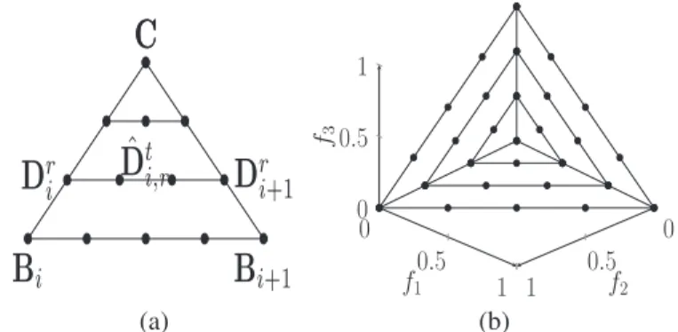
Any reference-direction-based MOEA cannot ignore the importance of the setting of reference directions (or weight vectors in [48]). Early MOEA/D algorithms employ a sys-tematic approach, developed by Das and Dennis [9], to generate H = p+MM−−11 reference directions on a unit sim-plex for M objectives, where p is the number of divisions
Fig. 1. Intersections of reference directions and a unit simplex. Reference (a) directions on the subsimplex Simp(i) and (b) directions (with 28 directions generated by three layers) in 3-D space.
considered along each objective coordinate. The systematic approach works well for a low-dimensional objective space, especially for bi-objective problems, where the number of reference directions can be arbitrarily designated. For high-dimensional problems, however, this approach will generate a large amount of reference directions if intermediate reference directions (which require p≥M) within the simplex are
pur-sued [13]. This inevitably pushes up the computational burden of MOEAs. To avoid such a situation, a two-layer (bound-ary and inside layers) approach for objectives over seven was proposed in [13] and [31], which uses the systematic approach to generate two reference direction sets: one set on the boundary layer and the other on the inside layer. Despite that the two-layer approach improves the generation of refer-ence directions, it still produces a large number of referrefer-ence directions for a high-dimensional objective space, which will be illustrated later.
To reduce these drawbacks, we present a k-layer reference direction generation approach. Since any reference direction should be sampled from a unit simplex, we can partition the unit simplex into a number of subsimplexes and then generate a set of diverse reference directions for each sub-simplex. First, we denote the central reference direction as C=(1/M, . . . ,1/M), and the ith extreme reference direction (the intercept on the ith axis) as Bi = (b1, . . . ,bM) where
bi =1 and bj=0 for all j=i, 1≤j≤M, 1≤i≤M. Thus, the unit simplex can be partitioned into M subsimplexes, each of which (denoted as Simp(i)) is bounded by points C, Bi, and Bi+1. In the following, we explain how to use our proposed k-layer approach to generate reference directions for the
sub-simplex Simp(i), and reference directions in other segments can be constructed in the same way.
For the subsimplex Simp(i), we first generate points on sides CBi and CBi+1. As illustrated in Fig.1(a), the rth reference
direction (denoted as Dri) within the line CBican be calculated as follows:
Dri =C+r
k(Bi−C) (1)
where r ∈ {1, . . . ,k}. This generates k reference directions (actually k layers from vertex C to the base BiBi+1) from the
central point to the ith extreme point. After that, we focus on calculating reference directions within the rth layer. Likewise, the tth reference direction within the line DriDri+1 on the rth
Algorithm 2 Reference_Generation()
1: Input: K (number of layers), M (number of objectives), N (archive size)
2: Output: W (reference direction set) 3: if M<3 then
4: Use Das and Dennis’s method [9] to generate W; 5: else
6: Generate extreme points Bi for i=1,· · · ,M, and the
central point C;
7: for i :=1 to M do
8: for r :=1 to K do
9: Calculate all points on the r-th layer by Eq. (2);
10: end for 11: end for 12: end if layer is computed by ˆ Dti,r=Dti+ t r+1 Dri+1−Dti (2) where t∈ {1, . . . ,r}. This generates r reference directions for the rth layer of Simp(i). Similarly, diverse reference directions in the rest of M −1 subsimplexes can be produced by the above method. At last, the constructed reference direction set
W comprises the central reference direction C, and reference
directions of each layer in each subsimplex.
It is easy to see that, for k layers, the total number (HMk) of reference directions for an M-objective problem is given by
HkM = M i=1 k r=1 r+k +1= Mk(k+3) 2 +1. (3)
For example, for M =3 and k =1, the reference directions are created on a triangle with vertices at(1,0,0),(0,1,0), and (0,0,1), including three midpoints of the sides of the triangle and an intermediate point at(1/3,1/3,1/3). Fig.1(b) presents a simple example of reference direction set generated by three layers. In this paper, for bi-objective problems, we use Das and Dennis’s systematic approach [9] to predefine a set of uniform reference directions, while for M>2, the k-layer approach is used. The generation of a predefined reference direction set is described in Algorithm2.
B. Offspring Reproduction and Objective Normalization
Reproduction (line 6 in Algorithm 1) is a step to create a new offspring population to update the parent population
P (which is actually regarded as the archive). Here, mating
selection plays a important role in reproduction. Each parent individual P1 ∈ P needs a mate P2 ∈ P to do reproduction.
SPEA/R employs a restricted mating scheme to select the mate
P2 for P1. Specifically, K candidates different from P1 are
randomly chosen from the parent population. Then, the can-didate minimizing the Euclidean distance (in objective space) to P1 can be screened as P2. K=20 is recommended in this
paper based on some preliminary experiments. The restricted mating scheme may help alleviate recombination issues in many-objective optimization, where recombining two distant
Algorithm 3 Objective_Normalization(Q) 1: Input: Q (combined population)
2: Output: Q (normalized population) 3: for i :=1 to M do
4: Compute the ideal point zimin:=minq∈Qfi(q);
5: Compute the worst point zimax:=maxq∈Qfi(q);
6: end for
7: for each member q∈Q do
8: Computed the normalized objective vector by Eq. (4);
9: Save the normalized q to Q;
10: end for
or very different parents is too disruptive and not likely to generate good children [13], [29].
After the production of the new offspring population P, SPEA/R then combines it and the parent population to form a population Q (line 7 in Algorithm1), which is used later to normalize the objectives of individuals (line 8 in Algorithm1). The normalization procedure is described in Algorithm 3. First, the ideal point zmin = (z1min, . . . ,zMmin) and the worst
point zmax =(z1max, . . . ,zMmax)are constructed from the
non-dominated set of the combined P and P, where zimin = min(fi(q))and zimax=max(fi(q)), q∈Q, i=1, . . . ,M. Then, the objectives of member q are translated as follows:
ˆ fi(q)= fi(q)−zimin zi max−zimin (4) where i ∈ {1, . . . ,M} and fˆi(q) denotes the ith normalized objective of member q.
C. Member Association and Fitness Assignment
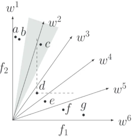
After mapping the objectives of members of Q into a unit hypercube, next we need to associate each member in the normalized population Q with a reference direction (line 10 in Algorithm1). The member association procedure is presented in Algorithm4. For each reference direction wi∈W, i∈ {1, . . . ,HMk}, we define a subregion, denoted asi, in the objective space, as follows:
i=ˆ F(x)∈f Fˆ(x),wi ≤ Fˆ(x),wj (5) where j∈ {1, . . . ,HkM}, x∈x,Fˆ(x)is the normalized objec-tive vector of x, and ˆF(x),wj is the acute angle between vectorsFˆ(x) and wj. Using this definition can easily identify a number of members residing in i, denoted as E(i), from the normalized population Q.
The idea of decomposing the objective space has also been employed in [7], [31], and [34]. In both [7] and [34], the objective space decomposition provides a way to approximate a small segment of the POF, while in [31], it is used for local density estimation and diversity maintenance.
The decomposition of objective space can facilitate fitness assignment, as shown in Algorithm5. In detail, each member a in E(i)is assigned a “local”1strength value S(a), representing 1The term local used here is to clarify the difference between our fitness
Algorithm 4 Associate(Q,W,i)
1: Input: Q (combined population), W (reference direction set)
2: Output: E(i)(individuals in the ith subregion)
3: for each q∈Q do 4: for each w∈W do
5: Compute the acute angle ˆF(q),w;
6: end for 7: Assignwˆ =w : argminw∈W ˆF(q),w; 8: Assignθq= ˆF(q),wˆ ; 9: Save q in E(wˆ); 10: end for Algorithm 5 Fitness_Assignment(E(i))
1: Input: E(i)(individuals in the ith subregion), Q (combined
population), W (reference direction set)
2: Output: FV (fitness values of members in E(i))
3: for each a∈E(i)do
4: Compute the “local” raw fitness R(a)using Eq. (7);
5: Estimate the density value D(a)using Eq. (8);
6: Compute the “local” fitness value FVl(a) := R(a)+ D(a);
7: Assign the final fitness value FV(a)using Eq. (10);
8: end for
the number of solutions it dominates in E(i)
S(a)=C({a∈E(i)|ab}) (6) where b∈E(i)and C(·)denotes the cardinality of a set. The local strength value is then used to calculate the local raw fitness R(a)of a member a in E(i), as follows:
R(a)=
b∈E(i),ba
S(b) (7)
where the local raw fitness depends on the strengths of its dom-inators in the same subregion. Note that, similar to SPEA2, the fitness is to be minimized here.
In the case where individuals in E(i)do not dominate each other, their raw fitness values will be zero and the above fit-ness assignment will make no sense. Fig. 2 presents such a situation, where both a and b are in the same subregion and they are nondominated individuals. Intuitively, a is bet-ter than b because it is closer to the associated reference direction (y-axis). Thus, individuals’ other information should be considered. We adopt an angle-based density estimation technique to discriminate between individuals having identi-cal raw fitness values. Each individual a∈E(i)has a unique angle value θa= ˆF(a),wi , which is actually the acute angle betweenFˆ(a)and the associated reference direction wi. Then, the density D(a)of individual a is estimated by
D(a)= θa θa+θm (8) where θm = max 1≤i≤Hk M min j=i(w
i,wj), i.e., the largest acute angle between two neighboring reference directions, is added to
Fig. 2. Influence of decomposed subregions on environmental selection. The gray area represents the subregion occupied by w2, i.e.,2, and the dashed lines are used to indicate d dominates c.
ensure that D(a)is smaller than one. The local fitness value of individual a, denoted as FVl(a), is composed of its raw fitness and density value, combined in the following form:
FVl(a)=R(a)+D(a). (9) This way, individuals with better local diversity and conver-gence will have higher final fitness. Thus, a is better than b in the case illustrated in Fig.2.
Despite great benefit for subregion diversity and local con-vergence, the local fitness assignment may impair global convergence if all individuals in i are dominated by indi-viduals in other subregions. To avoid this situation, individual
a is also assigned a “global” fitness value, denoted as FVg(a), which is actually the raw fitness in SPEA2 (see [53]). Besides, if a is the only member in i and dominated by individuals in other subregions, it should be given a chance to survive to the next generation. Thus, the final fitness of a, or FV(a), is calculated as
FV(a)=
FVl(a) ifi=1
FVl(a)+FVg(a) otherwise. (10) Considering again the example in Fig. 2, individual c is the only member in the associated subregion 2, but, it is domi-nated by d in another subregion. This means2might be an underexploited area in the objective space and the search in this area should be enhanced. Conventional Pareto-dominance-based techniques, e.g., NSGA-II and SPEA2, however, are likely to ignore or even simply abandon important individuals like c in this area. In contrast, the proposed fitness assignment rewards the isolated c at an attempt to attract other individuals toward the underexploited area. This way, the fitness assign-ment hopefully provides a good approximation to each region of the POF.
D. Environmental Selection
In the environmental selection (line 13 in Algorithm 1), the best N individuals that can balance diversity and convergence should be preserved. Here, we present a new environmental selection strategy, which is shown in Algorithm6. The strategy repeatedly selects an array (H) of individuals coming from
Algorithm 6 Environment_Selection(Q,W)
1: Input: N (population size), Q (combined population), W (reference direction set)
2: Output: P (new parent population). 3: Set P= ∅;
4: while C(P) <N do 5: Set H= ∅;
6: for each reference direction i∈W do 7: if E(i)= ∅then
8: Assignqˆ=q : argminq∈E(i)FV(q);
9: Saveq in H and remove it from Eˆ (i);
10: end if 11: end for
12: if C(P∪H) <=N then
13: P=P∪H;
14: else
15: Fill up P with the best N−C(P)individuals in terms of fitness from H;
16: end if 17: end while
each subregion, and copy the selected individuals to the new population P if the population size C(P) is not larger than
N. Otherwise, N−C(P)individuals from the last considered array are required to exactly fill up the new population. In this situation, the last array is sorted according individuals’ fitness and then the best N−C(P)individuals are copied to P.
It should be noted that SPEA/R adopts a diversity-first-and-convergence-second strategy to perform the environmental selection, which is different from most existing MOEAs. SPEA/R repeatedly gives each subregion priority to preserve the most promising individual in the subregion, so individu-als in the first loop (lines 6–11 in Algorithm 6) of selection have the highest diversity, and those in the second loop has the second highest diversity, and so on. This way, population diversity can be well maintained. Besides, promising individ-uals chosen from each subregion often have good fitness, so convergence is also soundly considered. The selection strategy can be further enhanced by elaborating niche count of each subregion when performing convergence selection (line 15 of Algorithm 6) for filling up the population P.
E. Computational Complexity of SPEA/R
The objective normalization (line 8 in Algorithm1) requires
O(MN) computations. In line 10 of Algorithm 1, associat-ing a combined population of 2N individuals to HMk reference directions takes O(MNHkM). Suppose that Li = C(E(i)), the number of individuals in the subregioni, thenH
k M
i=1Li=N. Thus, fitness assignment for E(i) (line 11 in Algorithm 1) requires O(ML2i) operations. For environmental selection, computational resources are mainly consumed by convergence selection. In Algorithm6, lines 6–11 require O(HMk) compar-isons and sorting (line 15) spends O(N log N). In this paper, the population size N depends on HkM, as N ≈HkM. On aver-age, the number of individuals in the ith subregion will be
Li =2N/HMk ≈2. Thus, the average complexity of one gen-erational cycle of SPEA/R is O(MN2). In the worst case, that is, all the 2N individuals get trapped into one subregion and other subregions do not contain any member, the computa-tional complexity reaches O(MN2), which is the same as the average complexity.
III. EXPERIMENTS ONMULTIOBJECTIVEOPTIMIZATION
As a starting point, SPEA/R is studied on multiobjective problems. The test problems used here are the MOP [34] test suite, which is a modification of ZDT [52] and DTLZ [15] but more difficult than its predecessors. Since SPEA/R uses a framework similar to MOEA/D-M2M [34], it will be interesting to make a comparison between them. Additionally, we also compared SPEA/R with a subproblem-constrained MOEA/D, i.e., MOEA/D-ACD [43], which is a recently devel-oped algorithm and has shown great promise for the MOP test problems. These three algorithms2 employ the recombi-nation operator [35], as suggested in MOEA/D-M2M [34]. For fairness, MOEA/D-ACD uses our reference direction initial-ization method. The population size was set to 100 (by the systematic approach [9]) and 313 (by our k-layer approach with k = 13) for bi- and three-objective problems, respec-tively. The maximum number of generation was set to 5000 for all the problems, and each algorithm was executed 30 inde-pendent runs for each problem. A detailed description of the MOP [34] test suite and the recombination operator [35] is provided in the supplementary material.
A. Performance Metrics
In our experimental studies, we adopt the following widely used performance metrics.
1) Inverted Generational Distance [34]: Inverted
genera-tional distance (IGD) can provide reliable information on both diversity and convergence of obtained solutions. Let PF be a set of solutions uniformly sampled from the true POF, and PF∗be the approximated solutions in the objective space, the metric measures the gap between PF∗ and PF, calculated as follows:
IGDPF∗,PF=
p∈PFd(p,PF∗)
|PF| (11) where d(p,PF∗)is the distance between the member p of PF and the nearest member of PF∗. The sizes of the uniformly sampled PF are 5000 and 5050 for two and three objectives, respectively.
2) Hypervolume [54]: The HV metric measures the size of
the objective space dominated by the approximated solutions
S and bounded by a reference point R=(R1, . . . ,RM)T that is dominated by all points on the POF, and is computed by
HV(S)=Leb ∪ x∈S f1(x),R1× · · · ×fM(x),RM (12) where Leb(A)is the Lebesgue measure of a set A. In our exper-iments, R is set to(2.0, . . . ,2.0)T unless otherwise stated, and 2The source codes of MOEA/D-M2M and MOEA/D-ACD are from http://www.cs.cityu.edu.hk/∼qzhang/publications.html.
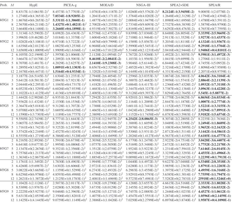
TABLE I
MEAN ANDSTANDARDDEVIATIONIGDANDHV VALUES ONMOP PROBLEMS
the exact HV metric (calculated by the WFG3algorithm [44]) is considered for comparison.
B. Results on Multiobjective Optimization
Table I presents the results of SPEA/R, MOEA/D-M2M, and MOEA/D-ACD, where mean and standard deviation val-ues of IGD and HV are reported and the best value for each problem is marked in boldface. The differences between the approximations are assessed by the Wilcoxon rank-sum test [45] at the 0.05 significance level, with the standard Bonferroni correction [1] to deal with the problem of the higher probability of type I errors in multiple comparisons.
The MOP [34] test suite contains seven hard-to-converge problems. In this suite, MOP4 is the only discon-nected problem, and MOP6 and MOP7 are two three-objective problems. Besides, MOP4–MOP7 are also diversity-resistant, which may be a big challenge to approximating well-distributed POFs if population diversity is not well maintained. TableIshows that, SPEA/R performs significantly better than MOEA/D-M2M on most of the test problems, in terms of IGD and HV. SPEA/R competes well with MOEA/D-ACD in terms of HV on these problems. Generally, SPEA/R mainly loses on the three-objective MOP6. On another three-objective MOP7, however, SPEA/R wins the comparison by a clear margin.
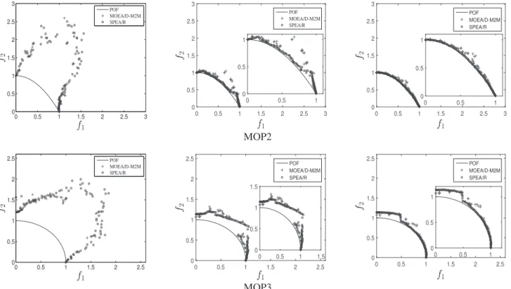
To have a better understanding of these algorithms’ performance, approximated POFs over 30 runs for the seven MOP problems are displayed in Fig. 3. As can be seen from the figure, SPEA/R, MOEA/D-M2M, and MOEA/D-ACD are all able to approximate the POF for the seven problems, but they perform differently in terms of convergence and diver-sity. Specifically, SPEA/R converges better than the other two algorithms on the first four bi-objective problems. On the two three-objective problems, i.e., MOP6 and MOP7, MOEA/D-M2M cannot achieve uniformly distributed approximations and misses some boundary regions of the POF. This means that MOEA/D-M2M may not be able to cover the whole POF in higher-dimensional problems. MOEA/D-ACD per-forms poorly in terms of diversity for MOP7, implying that adding constraints to subproblems is not enough to deal with hard-to-converge and diversity-resistant problems like MOP7. In contrast, SPEA/R maintains diversity well on both MOP6 and MOP7, although it does not fully converge to the POF in some runs.
3The latest implementation of WFG can be downloaded from http://www.wfg.csse.uwa.edu.au/hypervolume/.
The experiment on the MOP test suite shows that, SPEA/R and MOEA/D-M2M perform distinctly although both share some similar properties, e.g., decomposition of the objective space. The high performance of SPEA/R may be attributed to its good balance between diversity and convergence, which is achieved by our new proposed fitness assignment and environmental selection.
C. Comparison of Evolution Behavior With MOEA/D-M2M
Experimental results in the previous section have validated the performance of SPEA/R, but it is still not clear why SPEA/R performs better than MOEA/D-M2M on the MOP test suite despite their similar framework. To answer this question, we further compare the evolution behavior of these two algorithms on MOP2 and MOP3. To be more specific, the obtained approximations of three stages, i.e., the 50th (early stage), 500th (middle stage), and 1000th generation (late stage), are recorded, which are plotted in Fig. 4. It is clear to see from the figure that, SPEA/R maintains good popu-lation diversity all the time, whereas MOEA/D-M2M tends to partition population into several subpopulations far away from each other before the late stage, which means diversity between neighboring subpopulations is poorly controlled. As a consequence, MOEA/D-M2M takes more effort than SPEA/R to search unexplored regions before converging toward the POF and providing a good distribution of population, as illus-trated by the 1000th-generation approximation for MOP2. This reason can be also used to explain the poor distribution of MOEA/D-M2M on the three-objective MOP6 and MOP7 in the previous experiment. The figure also indicates that the use of diversity-first-and-convergence-second selection strat-egy can help SPEA/R to manage diversity and convergence well during the search.
IV. EXPERIMENTS ONMANY-OBJECTIVEOPTIMIZATION
Having had a good start on multiobjective optimization, SPEA/R is now examined on many-objective optimization. The section contributes to making a comparison of SPEA/R with state-of-the-art algorithms on many-objective problems.
A. Test Problems
The test problems used for algorithm comparison come from the WFG toolkit [21]. These problems contains a number of challenging characteristics, i.e., nonseparability, deception,
Fig. 3. Approximated POFs for MOP test problems over 30 runs. Left column: SPEA/R; middle column: MOEA/D-M2M; and right column: MOEA/D-ACD.
multimodality, biased attributes, and various POF geome-tries. For each WFG test problem, the number of objectives varies from two to twelve, which considers both multiobjective
and many-objective optimization. As recommended by the developers [21], the number of decision variables of all test instances is n = k + l, where k and l are the number
Fig. 4. Evolution behavior comparison between SPEA/R and MOEA/D-M2M for three stages on MOP2 and MOP3. Left: 50th generation; middle: 500th generation; and right: 1000th generation.
of position-related variables and distance-related variables, respectively. k = 2×(M−1) and l = 10 are used in this paper.
B. Compared Algorithms
Five popular or newly developed MOEAs are used for comparison in our experimental studies. They are MOEA/D [48], HypE [4], SPEA2+SDE [32], PICEA-g [42], and NSGA-III [13], and represent different classes of meta-heuristics. A brief description of each compared algorithm is given below.
1) MOEA/D4[48]: It is a representative of
decomposition-based algorithms. In this paper, PBI is adopted as the aggregation function for MOEA/D because it is empir-ically proved to be more effective than other decom-position methods for many-objective optimization in a recent study [13], and normalization [48] is used for scaled problems.
2) HypE5 [4]: It is a representative of indicator-based
MOEAs, which employs the HV metric as an indicator in the environmental selection. In HypE, the fitness value of a solution is determined by not only its own HV con-tribution but also the HV concon-tribution shared with others. Additionally, for the sake of computational complexity, HypE uses Monte Carlo simulation to approximate the exact HV values.
4The code of MOEA/D is fromhttp://dces.essex.ac.uk/staff/qzhang/. 5The code of HypE is fromhttp://www.tik.ee.ethz.ch/pisa/.
3) SPEA2+SDE6 [32]: This method introduces a density
estimator that considers both distribution and conver-gence information of individuals to increase the selection pressure in many-objective optimization. SPEA2+SDE has shown to be very promising for MaOPs [32]. 4) PICEA-g7[42]: It introduces a new concept of PICEA,
which coevolves a family of decision-maker preferences together with a population of candidate solutions, for many-objective optimization. PICEA-g is an implemen-tation of such a concept, where preferences gain higher fitness if it is satisfied by fewer solutions, and solu-tions gain fitness by meeting as many preferences as possible.
5) NSGA-III8 [13]: It is an upgraded version of the most
popular dominance-based NSGA-II algorithm, where a number of supplied reference points is used as a guideline for handling MaOPs. The basic framework of NSGA-III remains similar to NSGA-II, except that it maintains population diversity by niche preservation.
C. Parameter Settings
The parameters of the six MOEAs considered in the experiments are referenced from their original papers. 6The source code of SPEA2+SDE can be downloaded from http://www.brunel.ac.uk/∼cspgmml1/home.html.
7The source code of the PICEA-g algorithm can be downloaded from http://www.sheffield.ac.uk/acse/staff/rstu/ruiwang/index.
8The source code of NSGA-III (version 1.1) can be downloaded from http://web.ntnu.edu.tw/∼tcchiang/publications/nsga3cpp/nsga3cpp.htm.
TABLE II
POPULATIONSIZE FORDIFFERENTALGORITHMS
USING THEk-LAYERAPPROACH
Some key parameters in these algorithms were set as follows.
1) Reproduction Parameters: All the algorithms used the simulated binary crossover and polynomial muta-tion [13] as their genetic operators. The crossover probability was pc=1.0 and its distribution index was ηc = 20. The mutation probability was pm =1/n and its distributionηm=20.
2) Population Size: The population sizes (N) of different algorithms are presented in Table II. The population sizes of all the algorithms except MOEA/D were set as 4HMk/4, which is the smallest multiple of four not smaller than HMk, according to the suggestion in [13]. In other words, HypE, PICEA-g, and SPEA2+SDE use the same population size settings as NSGA-III and SPEA/R. 3) Stopping Criterion and the Number of Executions: Each algorithm was terminated after a prespecified number of generations. To be specific, for WFG problems, each algorithm stops after 300, 600, 1000, 1500, and 2000 generations for 2-, 3-, 5-, 8-, and 12-objective cases, respectively. Additionally, each algorithm was executed 30 independent times on each test instance.
D. Experimental Results and Analysis
The performance measures for quantifying the performance of the compared algorithms in this section are IGD [13] and HV [54]. Note that, the POF points used for computing IGD here are a set of target points on the POF associated with ref-erence directions, as suggested in [13]. For HV computation, the ith objective of the reference point used is 2i+2 for all the WFG problems, and the HV values presented in this paper are all normalized to [0,1] by dividing Mi=1(2i+2). The IGD
and HV values of six algorithms on nine WFG test problems are presented in Tables IIIandIV, respectively.
The WFG1 problem mainly examines whether an MOEA can handle bias and mixed POF shapes. Both IGD and HV metrics indicate that PICEA-g is more suitable for this kind of problem than the other compared algorithms. SPEA/R competes well and even outperforms the others for relatively low-dimensional cases. But, it is defeated by NSGA-III on the 12-objective WFG1 in terms of the HV metric.
WFG2 challenges algorithms’ ability to locate all dis-connected POF segments and handle nonseparable vari-able dependencies. For this problem, all the algorithms can achieve impressive performance in low-dimensional cases, and SPEA/R wins by a clear margin. However, when the num-ber of objectives is over five, the performance of MOEA/D
and NSGA-III degrades sharply whereas SPEA/R continues to yield good results. SPEA/R wins in the eight-objective case and can compete with HypE and SPEA2+SDE in the 12-objective case, as indicated by both IGD and HV metrics. This means SPEA/R can deal with disconnectivity.
WFG3 features a degenerated and linear POF shape and its variable is nonseparable as well. For this problem, while SPEA/R performs best for the two-objective case, its performance degrades sharply when the number of redun-dant objectives increases, which is also the case for the other algorithms except PICEA-g. PCIEA-g is roughly the best per-former for this problem because it generates nondominated reference points in the objective space to guide the search in every generation. The other algorithms to a certain extent try to spread population over the whole objective space for the sake of diversity, leading to a very limited number of points on the degenerated POF. Despite that, SPEA/R out-performs MOEA/D and NSGA-III and out-performs competitively with SPEA2+SDE for the 8- and 12-objective cases. This may be because fitness assignment in SPEA/R favors nondominated solutions.
The problems WFG4 to WFG9 have an identical hyperel-lipse surface, but they differ in some other characteristics. To be specific, WFG4 introduces multimodality to test algorithms’ ability to escape from local optima, and WFG5 is a decep-tive problem, and the difficulty lies in the large “aperture” size of the well/basin leading to the global minimum. WFG6 has a significant nonseparable reduction, and WFG7–WFG9 all introduce some bias to challenge algorithms’ diversity, but WFG8 and WFG9 are nonseparable. Also, variable linkages in WFG8 are much more difficult than that in WFG9.
For WFG4–WFG9, SPEA/R wins nearly all the tested cases in terms of IGD and HV, showing high ability to deal with a number of considered characteristics in these prob-lems. Considering the HV metric, PICEA-g also achieves very competitive results on these problems, and outperforms or compares well with SPEA/R in some cases. However, none of the other algorithms can compete with SPEA/R.
The above experimental studies show that the tested algo-rithms’ performance can be influenced by at least two factors, i.e., problem characteristics and the number of objectives. Clearly, degeneration in WFG3 poses a big challenge to reference-based algorithms, i.e., MOEA/D, NSGA-III, and SPEA/R, as they roughly pursue diversified population over the whole objective space. On the other hand, an increase in the number of objectives to some extent influences all the tested algorithms. MOEA/D is the most influenced one among six algorithms, which experiences a sharp drop when the num-ber of objectives increases from five to twelve, as indicated by the deterioration of IGD and HV. This is consistent with some recent studies [31], [47]. This observation shows MOEA/D struggles to solve difficult many-objective WFG problems.
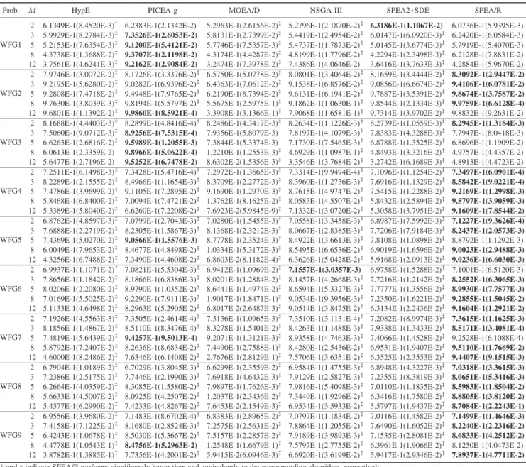
To understand why SPEA/R generally performs better than the other algorithms, we graphically plot the parallel coor-dinates (normalized by the nadir point) of final solutions obtained by each algorithm for the 12-objective WFG4 in Fig. 5. For the inspection of parallel coordinates for sev-eral other WFG instances, the interested readers are referred
TABLE III
MEAN ANDSTANDARDDEVIATIONIGD VALUESOBTAINED BYSIXALGORITHMS FORWFG PROBLEMS
to the supplementary material. The figure clearly shows that SPEA/R is able to obtain a good spread of solutions in the entire range of the POF (fi∈[0,2i], for all i), whereas HypE, PICEA-g, MOEA/D, and NSGA-III miss some part of the POF. Due to effective density estimation, SPEA2+SDE shows very competitive diversity performance, but it does not cover well the entire POF. Thus, we can conclude that the outper-formance of SPEA/R over the other algorithms results largely from its sound diversity maintenance and its effective fitness assignment capable of driving population toward the POF.
V. INVESTIGATIONS ANDDISCUSSION
A. Comparison of Different Reference Direction Generation Approaches
As the population size (Popsize) of MOEAs is closely asso-ciated with the amount of reference directions, we compare
our proposed k-layer approach with the systematic approach used in MOEA/D [48] and the two-layer approach used in NSGA-III [13] in terms of required Popsize for different num-bers of objectives. Since the two-layer approach is an improved version of the systematic approach for generating reference directions in the case of seven or more objectives, we just need to compare our k-layer approach with the former and the latter in low-dimensional cases and high-dimensional cases, respectively.
The results are given in Fig.6, where for each approach, 20 different levels of Popsize are continuously sampled. Clearly, for three objectives, the systematic approach shows better
Popsize settings than the k-layer approach. However, when M is increased from 5 to 7, the k-layer approach has more
choice to set the population size in the range of 10–1000. For eight-objective problems, the two-layer approach works slightly better than the k-layer method, but for much higher
TABLE IV
MEAN ANDSTANDARDDEVIATIONHV VALUESOBTAINED BYSIXALGORITHMS FORWFG PROBLEMS
objectives, the Popsize generated by the two-layer approach grows very fast, particularly for 30 objectives. In this case, the k-layer approach gives more options to configure a desir-able population size. Thus, in comparison with the other two approaches, the k-layer approach appears more suitable for generating a reasonable size of population for MaOPs with a large number of objectives.
The uniformity of reference sets generated by dif-ferent approaches is investigated on difdif-ferent levels of population size and various number of objectives. The most widely used discrepancy measure, i.e., centered L2
-discrepancy [20], is employed to measure the uniformity of generated reference sets. Comparisons between the simplex-lattice design [13], [48] and our k-layer approach is provided in the supplementary material. The comparisons indicate that the k-layer approach can generate a reference set that covers the whole reference vector space in a good manner.
B. SPEA/R Versus NSGA-III
SPEA/R and NSGA-III share some similarities in the way that they keep diversity with the aid of reference direc-tions. Besides different methods for constructing reference directions, there are several key differences between them, resulting in distinct search behaviors. First, SPEA/R introduces a restricted mating selection to enhance reproduction instead of random selection, which is very helpful for many-objective optimization where distant parents are not likely to generate good solutions. Second, SPEA/R uses a simple normalization method based on the worst value of each objective, whereas normalization in NSGA-III requires intercept computation and hyperplane construction, which are computationally expensive, particularly for many-objective problems, and NSGA-III may also have difficulty in hyperplane construction due to dupli-cate extreme points. Third, niche preservation strategies are different in SPEA/R and NSGA-III. Whenever preserving a
Fig. 5. Parallel coordinates of final solutions obtained by six algorithms for the 12-objective WFG4 instance. (a) HypE. (b) PICEA-g. (c) MOEA/D. (d) NSGA-III. (e) SPEA2+SDE. (f) SPEA/R.
Fig. 6. Comparison of the population size required by different methods. (a) Systematic approach and k-layer approach for low-dimensional cases. (b) Two-layer approach and k-layer approach for high-dimensional cases.
member from the last front considered, NSGA-III tries to repeatedly identify reference directions having the worst niche count, which is the number of members associated with these reference directions that has been preserved in higher fronts (the higher, the better). This procedure is computationally inefficient. Furthermore, this strategy may result in some iso-lated but promising members in lower fronts being abandoned if nondominated sorting terminates before considering these lower fronts, implying that population diversity in NSGA-III is still not well maintained. In contrast, as illustrated in Section III-C, SPEA/R intentionally gives higher priority to diversity than convergence when performing environmental
selection, leading to impressive performance on MOP prob-lems, and the niche preservation strategy in SPEA/R has also been further validated on multiobjective and many-objective WFG problems.
Generally, normalization and niche preservation are all aimed to help keep diversity. To understand the second and third differences, we tested SPEA/R and NSGA-III on dis-parately scaled three-objective WFG5. That is, the objectives
f1–f3 are multiplied with 5, 52, and 53, respectively. Fig. 7
plots approximated POFs of the median and worst IGD values over 31 runs, showing that the simple normalization method used in SPEA/R can deal with scaling objectives and the
Fig. 7. Approximated POFs for scaled WFG5. Top: the median approxima-tion and bottom: the worst approximaapproxima-tion.
new diversity-first-and-convergence-second strategy is capable of providing a uniform distribution of solutions. NSGA-III, however, struggles to solve the scaled WFG5. In the median case of NSGA-III, the intercept-based normalization is able to diversify points over the whole POF but the niche preser-vation cannot provide a good distribution. In the worst case, NSGA-III drives the majority of points toward the f1f3 plane, and misses a large part of the POF. One reason for this is that NSGA-III tends to preserve members in higher fronts that have better convergence, and less-converged isolated ones in lower fronts are likely to leave unconsidered, leading to poor diver-sity during the search. Therefore, NSGA-III cannot compete with SPEA/R in terms of diversity.
C. Influence of Fitness Assignment and Niche Preservation
Although Section III-C has revealed that good popula-tion diversity contributes to the performance of SPEA/R, in this section we try to unveil more reasons behind the high performance of SPEA/R.
Fitness assignment and diversity preservation are the core of SPEA/R, which control the balance between convergence and diversity. To understand why our strategy yields high performance, we further design three other SPEA/R variants that use different strategies. The first one, called SPEA/R-A, removes global fitness from (9) when calculating individuals’ fitness. Instead of removing global fitness, the second vari-ant, i.e., SPEA/R-B, removes local fitness, so an individual’s final fitness is composed of global fitness and density. The third variant (named SPEA/R-C) allows individuals with the highest fitness to enter into the next generation in environ-mental selection. Thus, SPEA/R-A favors diversity whereas SPEA/R-C favors convergence, and SPEA/R-B does not con-sider local convergence. The variants are compared with the original SPEA/R on seven MOP problems and nine WFG problems with 2, 3, 5, 8, and 12 objectives. The HV results obtained by each algorithm for a total of 52 instances are presented in our supplementary material, and only statisti-cal testing result is given in Table V, which is based on the
TABLE V
STATISTICALDIFFERENCEBETWEENSPEA/RANDTWOVARIANTS
Fig. 8. IGD metric against the number of generations for two instances: SPEA/R (solid); SPEA/R-A (dashed); and SPEA/R-B (dotted). (a) MOP3. (b) WFG4.
Wilcoxon signed-rank test [45] at the 0.05 significance level with Bonferroni correction. In the table, the signs “B,” “E,” and “W” represent SPEA/R is significantly better, equivalent to, and worse than the compared variant, respectively.
It is clear that, SPEA/R generally performs better than the other variants. Specifically, SPEA/R outperforms SPEA/R-A in a number of cases, indicating that the use of global fitness is a good choice for SPEA/R in some situations. The comparison between SPEA/R and SPEA/R-B shows that the use of local fitness does not make a big difference but may help SPEA/R achieve slightly better performance for a few instances. For SPEA/R-C, the lack of diversity maintenance induces a sig-nificant lag behind SPEA/R. This observation further confirms that the high performance of SPEA/R is mainly due to sound diversity preservation.
Since SPEA/R, SPEA/R-A, and SPEA/R-B differ only in fitness assignment, one would wonder why SPEA/R works better (though not significantly better in most cases) than the other two variants. To investigate this, we plot the mean IGD curves of these variants against the first 300 genera-tions on MOP3 and two-objective WFG4, as shown in Fig.8. It can be observed that SPEA/R converges fastest, followed by SPEA/R-B, and SPEA/R-A ranks last. SPEA/R is better than SPEA/R-A because adding local fitness can strengthen discrimination between individuals so that more-converged individuals can be preserved. In contrast, without the use of global fitness, SPEA/R-A converges relatively slower than SPEA/R and SPEA/R-B. This illustrates that the joint use of global fitness and local fitness can speed up the search pro-cess, although not very significantly. However, we should point out that there is no much difference between SPEA/R and SPEA/R-B in high-dimensional problems. This is because the local fitness value will be zero when the majority of individ-uals are nondominated in high dimensions. In other words, SPEA/R may degenerate to SPEA/R-B in this situation.
D. Influence of Restricted Mating
Restricted mating selection is somewhat similar to the con-cept of neighborhood used in MOEA/D, in which close parents
TABLE VI
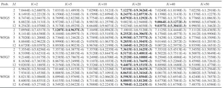
MEAN ANDSTANDARDDEVIATIONHV VALUESOBTAINED BYSPEA/R WITHDIFFERENTK VALUES FORFOURWFG PROBLEMS
are likely to generate good offspring. It has a key parameter K, i.e., the number of parent candidates, and the influence of this parameter is investigated on four WFG problems. Table VI
reports the HV values obtained by SPEA/R with different set-tings of K. It can be observed that, K = 20 (10%–20% of population size) yields better results than the other settings for all the cases except the 8- and 12-objective WFG5 and the two-objective WFG6. Particularly, for many-objective prob-lems, e.g., the 8- and 12-objective cases, there is a noticeable improvement on the HV metric when K is increased from 2 to 20. This means proper restricted mating can benefit population reproduction, thereby promoting algorithms’ performance for many-objective optimization.
The above experiment has shown that proper restricted mat-ing is good for population reproduction. However, we should point out that, restricted mating can be used only when popula-tion diversity is well maintained. This is because, if populapopula-tion individuals are not well distributed, then restricted mating can cause overexploitation in overcrowded regions so that isolated regions may be left under-explored or even unexplored, result-ing in a further deterioration of population diversity. This has been illustrated in Section V-C, where the overlook of diver-sity maintenance makes SPEA/R-C significantly worse than SPEA/R although restricted mating has been employed there.
E. Performance of SPEA/R on Problems With More Objectives
SPEA/R has the advantage of population diversity main-tenance so that it can handle high-dimensional problems. To further investigate whether this advantage can deal with prob-lems with more objectives, we tested SPEA/R on WFG4 with 20 and 40 objectives. This means the difficulty of the problem is massively increased as nearly all population members are nondominated with respect to each other. The population size was set to 280 and 560 for 20 and 40 objectives, respectively. Due to the increase of the difficulty of the problem, SPEA/R should be given more computational resources. Hence, the
maximum number of generations was set to 3000 and 5000 for 20 and 40 objectives, respectively.
Fig. 9 shows the normalized parallel coordinates of final solutions obtained by SPEA/R for two instances. Clearly, on both 20 and 40 objectives, SPEA/R can still obtain a set of diverse solutions in the entire range of the POF. Thus, the proposed diversity-first-and-convergence-second selection strategy in SPEA/R is very promising for solving many-objective problems.
F. More Discussions
It has been well recognized that convergence and diver-sity are two main but hard-to-balance goals in designing MOEAs. Any bias toward one goal will inevitably aggravate the other. In many-objective optimization the balance between them is still of great importance. However, when handling MaOPs, most MOEAs inherit elitist preservation from their counterparts of low-dimensional optimization that emphasizes nondominated solutions in the population, resulting in very lit-tle room left for diversity maintenance. Even if these MOEAs did not intentionally emphasize convergence, they could not elude the fact that an increasingly large fraction of popula-tion becomes nondominated with an increase in the number of objectives. In other words, they perform environmental selec-tion in a convergence-first-and-diversity-second manner. As a result, when the MOEAs are applied to high-dimensional optimization, there will be a large number of nondominated individuals after the convergence-first selection, and diver-sity preservation will be performed only on the nondominated individuals. Correspondingly, some regions occupied by dom-inated individuals will be scarcely explored, and diversity preservation becomes of limited use in this case. In con-trast, SPEA/R adopts a diversity-first-and-convergence-second strategy to perform environmental selection, at an attempt to maximize population diversity and strengthen exploitation
Fig. 9. Parallel coordinates of final solutions obtained by SPEA/R for WFG with (a) 20 and (b) 40 objectives.
in less-converged regions during the search. Our experi-ments have shown its promise for both multiobjective and many-objective optimization.
However, we may wonder why SPEA/R can work well on problems with over 12 objectives, where nearly all individ-uals (over 95% of population) are nondominated [23]. This means, in this situation, the diversity-first-and-convergence-second strategy in SPEA/R has no advantage over other MOEAs in diversity preservation because there is hardly any region that can be occupied by very few dominated individuals. There is no doubt that, when population is randomly gener-ated, the fraction of dominated individuals is close to zero for ten objectives and over [23]. But, what if the population is a combination of parent and offspring populations, which is the case with MOEAs? To investigate this, we consider the search behavior of SPEA/R on the 12-objective WFG5 over 2000 generations. In every generation, SPEA/R distributes a com-bined population toward HMk subregions (which equals the total number of reference directions) of the objective space, and the number (Nd) of subregions in which only dominated solutions reside is recorded. Fig.10shows the relative frequency of dif-ferent Ndvalues over 2000 generations. Clearly, in the majority of generations dominated solutions do not solely occupy any subregions. In this situation, dominated solutions make little contribution to diversity as nondominated solutions covers all subregions of the evolving population. However, there are also over 20% generations in which some subregions are occupied by dominated but not nondominated solutions. In this case, dominated solutions make a difference to population diversity. Additionally, we also compute the percentage of domi-nated solutions in the combined population of every gen-eration of SPEA/R for a single run, as shown in Fig. 11. It can be observed from the figure that, there is still a noticeable proportion of dominated solutions in the com-bined population before the population converges to the POF. All these observations clearly confirm that preservation of dominated solutions for diversity promotion through the diversity-first-and-convergence-second strategy is still benefi-cial to SPEA/R when handing high-dimensional problems.
Fig. 10. Relative frequency of the number of subregions occupied only by dominated solutions.
Fig. 11. Percentage of dominated solutions in every generation of SPEA/R for 12-objective WFG5.
On the other hand, Fig. 11 can also be used to explain why the compared MOEAs in this paper cannot compete with SPEA/R. As shown in this figure, there are at least