Computationally efficient approximation for the double bootstrap mean bias correction

(1)

Volume 31, Issue 3

Computationally efficient approximation for the double bootstrap mean bias

correction

Rachida Ouysse

The University of New South Wales

Abstract

We propose a computationally efficient approximation for the double bootstrap bias adjustment factor without using the inner bootstrap loop. The approximation converges in probability to the population bias correction factor. We study the finite sample properties of the approximation in the context of a linear instrumental variable model. In identified versions of the model considered in our Monte Carlo experiments, the proposed approximation leads to estimators with lower variance than those based on the double bootstrap and, lower adjusted mean-squared error than estimators based on the single bootstrap. Evidence from the experiments we consider suggests that the bootstrap is less effective in reducing the bias when the instrumental variable is weak and endogeneity is strong.

The author is very grateful to the associate editor and anonymous referee for their helpful comments which helped improve the quality of the paper.

Citation: Rachida Ouysse, (2011) ''Computationally efficient approximation for the double bootstrap mean bias correction'', Economics

(2)

Computationally efficient approximation for the double

bootstrap mean bias correction

Rachida Ouysse

∗

University of New South Wales

Sydney, Australia

Abstract

We propose a computationally efficient approximation for the double bootstrap bias adjustment factor without using the inner bootstrap loop. The approximation converges in probability to the population bias correction factor. We study the finite sample properties of the approximation in the context of a linear instrumental variable model. In identified versions of the model considered in our Monte Carlo experiments, the proposed approximation leads to estimators with lower variance than those based on the double bootstrap and, lower adjusted mean-squared error than estimators based on the single bootstrap. Evidence from the experiments we consider suggests that the bootstrap is less effective in reducing the bias when the instrumental variable is weak and endogeneity is strong.

KEYWORDS: Bias function; population and sample moments; true data generating process; empirical distribution; Monte Carlo simulation

(3)

1 Introduction

Many econometric estimators although consistent in large samples have small sample bias. The bootstrap is a simulation-based alternative to asymptotic approximation used to correct for finite sample bias for the purpose of point estimation and/or inference.

Advances in statistical theory show that iterating (pre-pivoting) the bootstrap principle brings yet further improvements upon the single bootstrap. Beran (1988) argues that pre-pivoting reduces the dependence between the probability distribution of the resample and the unknown data generating process. Therefore, resampling reinforces the conditions under which the bootstrap performs the best: pivotal or asymptotically pivotal statistics. As a result, the double bootstrap has typically higher order accuracy than the ordinary single bootstrap and the bootstrap can be iterated to reduce the bias by a factor of O(n−1₎

suc-cessively. See among others Beran (1988, 1987, 1990), Hall (1992, 1986), Hall and Martin (1988), Lee and Young (1999) and Shi (1992).

These refinements come with a heavy computational cost due to the increasing com-putational intensity of compounded sampling. This has prompted a number of authors to develop computationally efficient and cheaper alternatives to eliminate the need for nested levels of resampling. Much of the literature is however concerned with ways to generate fast approximations to the P value and quantile functions. To the best of our knowledge, this paper is perhaps the first to address the computational efficiency of approximating the bias function.

The technique of this paper adapts thefast double bootstrap of Davidson and MacKinnon (2002b, 2007) and the warp-speed method of Giacomini et al. (2007) for approximating the rejection and coverage probabilities of bootstrap tests and confidence intervals to the problem of approximating the bootstrap bias. The approximation requires only twice as many computations as what is usually needed to perform the single bootstrap. We show an optimality result which holds under general conditions and does not require an asymptotic pivot.

The statistical properties of the proposed fast approximation are examined in a linear instrumental variable framework through a Monte Carlo analysis. The results in our exper-iments show that the fast approximation achieves significant bias reduction over the single bootstrap without the increased variance and the computational cost of the double bootstrap. We use the following notation throughout the paper: Eµis the mathematical expectation

under the data generating process (DGP ) µ, Vµ is the variance under the DGP µ, the

indicator function 1{x} takes the value 1 if the statement in its argument is correct and 0 otherwise.

2 Bootstrap methods for bias correction

LetX1, X2, ... be a sequence of stationary random variables generated from a data

generat-ing process µ0 with unknown joint probability distribution F0 and possible indexed by an

(4)

processµ0 ofXwith realizationXn = (X1, X2, ..., Xn). Letbµbe the data generating process

(DGP ) governed by some estimateFbof the empirical distribution implied byXn_{. We choose}

the standard uniform Fb(y) = _n1 P_in₌₁1{Xi ≤y}.

Many statistical problems can be formulated as specifying the statistical properties of the random variable Rn(Xn, θ(µ0)) such as its probability distribution function, moments and

quantile functions. The bootstrap uses a nonparametric estimate Fn of F0 to approximate

the distribution of Rn using R∗n=Rn(Xn, Fn).

The bootstrap principle approximates the sampling distribution ofRn(Xn, θ(µ0)) by the

bootstrap distribution ofRn(X∗n, θ(µb)), whereX∗nis an IID random sample of sizendrawn

with replacement from the original sample Xn _using _F

n. We use µb∗ to denote the data

generating process indexed by the bootstrap empirical distribution Fb∗ defined in analogous way as Fb, that isFb∗(y) = 1 n Pn i=11(X ∗ i ≤y).

2.1 The single bootstrap

To fix ideas, consider the root function Rn(Xn, θ(µ0)) = θ(µb)− θ(µ0), where θ(µb) is a

consistent estimator for θ(µ0). The theoretical bias β(µ0) is defined by the population

equation,

Eµ0[Rn(X

n

, θ(µ0)) +β(µ0)] = 0. (1)

The bootstrap estimateβ(_bµ) for the bias correctionβ(µ0) is defined by the bootstrap version

of (1),

E

b

µ[Rn(X∗n, θ(µb)) +β(µb)] = 0. (2)

Definition 1 The single bootstrap bias corrected estimator is defined as θbbc =θ(µb) +β(µb),

where β(µ_b) =θ(_bµ)−E

b

µ[θ(bµ∗)].

The single bootstrap algorithm. Given the original sample Xn_, _B _{bootstrap resamples}

X∗_bn, b = 1,· · · , B are randomly drawn from the DGP _bµ. For each bootstrap resample, the sample valueθb∗_b of the statistic θ(µ_b∗) is computed. A Monte Carlo estimate ofβb∗ for the theoretical bias β(µ_b) is calculated using

b β∗ = θ(µ_b)− 1 B B X b=1 b θ∗_b. (3)

The amount of uncorrected bias in θbbc is of order O(n−2); an improvement to the original

estimator θ(µ_b) which has a bias of order O(n−1_{). For a discussion of the bootstrap}

refine-ments, see among others Horowitz (2001), Hall and Horowitz (1996), Efron (1987, 1979) and Efron and Tibshirani (1986).

(5)

2.2 The double bootstrap

Beran (1988, 1987) propose the idea of repeated pre-pivoting by mapping a test statisticτn,j

into a new test statistic τn,j+1 where τn,0 is the original sample statistic and τn,1 is the first

bootstrap statistic. The null distribution ofτn,j is less strongly dependent on the parameters

indexing the unknown probability distribution F0. Hall (1986) shows that the accuracy of

the approximation using the jth _{(iterated) bootstrap critical value is of order} _O₍_n−(j+1)/2_).

Furthermore, Shi (1992) shows that the double bootstrap principle can be used without the need of a pivot.

In this section, we use follow Shi (1992), Hall (1992) and Davison and Hinkley (1997) to derive the double bootstrap equation for mean bias correction.

Let X∗∗n be a (second level) IID random resample of size n drawn with replacement from the first level sample X∗n _using _F

n. We use µb∗∗ to denote the data generating process

indexed by the empirical distribution of X∗∗n_.

The likelihood function of θ(µ_b) differs from the conditional density function of θ(µ_b∗), therefore the bootstrap bias estimator β(µ_b) in Definition 1 does not necessarily satisfy the population equation in (1),

Eµ0[Rn(X

n_{, θ}₍_µ

0)) +β(µb)] 6= 0. (4)

Using Davison and Hinkley (1997) notation, to adjust for the deviation from the population equation, a perturbation or adjustment factor is introduced in the form of b(µ, γ_b (µ0)) such

that,

Eµ0[Rn(X

n_{, θ}₍_µ

0)) +b(bµ, γ(µ0))] = 0. (5)

For an additive perturbation, the adjustment takes the formb(_bµ, γ(µ0))≡β(µb) +γ(µ0).

The bootstrap estimate for γ(µ0) is generated through the bootstrap version of (5): E

b

µ[Rn(X∗n, θ(µb)) +b(µb∗, γ(bµ))] = 0. (6)

Notice that b(µ_b∗, γ(µ_b)) requires a second level bootstrap to estimate β(µ_b∗). The bootstrap estimates for β(_bµ∗) and b(µ_b∗, γ(µ_b)) are defined by the sample equations:

E b µ∗[R_n(X∗∗n, θ(µb∗)) +β(µb∗)] = 0, (7) E b µ[Rn(X∗n, θ(µb)) +b(bµ∗, γ(µb))] = 0. (8)

Combining equations (7) and (8) and assuming an additive adjustment, the double boot-strap estimate of the adjustment factorγ(µ_b) is rewritten as

γ(µ_b) = Eµ_b[β(µb)−β(µb∗)], (9)

= Eµ_b{Eµb

∗[θ(µb∗∗)−θ(µb∗)]−[θ(µb∗)−θ(µb)]}. (10)

Definition 2 The double bootstrap bias estimation γ(_bµ) in equation (9) defines a double bootstrap estimator θbdbc,

b

(6)

The double bootstrap algorithm. From the original sample Xn_{, draw} _B

1 bootstrap resamples

X∗n

b , b = 1,· · · , B1 using the empirical distribution Fbn. For each resample X∗bn, (i)

com-pute the bootstrap realized value bθ∗_b of θ(_bµ∗_b), (ii) draw B2 second level bootstrap resamples

X∗∗_b,jn, j = 1, .., B2from the bootstrap empirical distributionFbb∗, and (iii) compute the second

level bootstrap estimators θb∗∗_b,j, j = 1, .., B2. For b = 1,· · · , B1, compute an estimate βbb∗ for

the second level bias adjustment β(µ_b∗) as:

b β_b∗ =θb∗_b − B2 X j=1 b θ_b,j∗∗/B2.

The Monte Carlo estimate of the double bootstrap bias adjustment in equation (9), denoted

b γ∗∗, is computed as b γ∗∗ = βb− 1 B1 B1 X b=1 b β_b∗. (11)

The double bootstrap doesn’t come cheap. The algorithm makes a total of B1(B2 + 1)

(= 249500 for B2 = B1 = 499) visits to the statistic R(X∗n, θ(µb)). This indeed becomes

quickly computationally cumbersome depending on the model and the estimation method despite the increase in computational power.

3 Fast methods for approximating the

P value

Let us consider the case of estimating the rejection probability and P value of bootstrap tests. Using the notation of Giacomini et al. (2007), consider the root functionRn(Xn, θ(µ0)) with

sampling distribution Jn(·, F) and limiting distribution J(·, F). The bootstrap principal

approximates the limiting distribution J(x, F) using the bootstrap distributionJbn(x, Fn∗)≡

P_n∗{Rn(Xk∗n, θ(bµk))≤x}.

Standard Monte Carlo experiment.

For each Monte Carlo sample Xn_k (with DGP _bµk), draw B IID bootstrap samples from bµk.

The bootstrap estimate forJbn,k(·, Fn∗) is computed usingJ

∗ n,B,k(x)≡B −1PB b=1Rn(X n∗ k , θ(µbk))≤

x. The quantileq_n,B,k∗ is then computed by inverting J_n,B,k∗ (·). For a left-tail bootstrap test, the empirical rejection probability is approximated using

RPn,B,K =K−1 K

X

k=1

1Rn(Xnk, θ(µ0))≤qn,B,k∗ (α) . (12)

The standard Monte Carlo method requiresB·Kcomputations of the root functionRn(X∗n, θ(µb)).

Applying the law of large numbers, J_n,B,k∗ converges toJbn,k(·, Fn∗). Let qb∗(α) be theα

(7)

Giacomini et al. (2007)), RPn,B,K converges to

RP =P

b

µ{Rn(Xn, θ(µ0))≤qb∗(α)}. (13)

Note that the rejection probability in equation (12) also corresponds to the bootstrap P value. This can be seen by rewriting (13) as,

RP =P

b

µ{Pbµ

∗[R_n(X∗∗n, θ(bµ∗))≤R_n(Xn, θ(µ₀))]≤α} (14)

Warp/fast algorithm.

For each Monte Carlo sample Xn

k, k = 1,· · · , K, draw B = 1 bootstrap resample X

∗n k and

compute the root Rn(Xnk∗, θ(bµk)). Giacomini et al. (2007) provide conditions under which

the distribution functionJbn(x, Fn∗) can be approximated using,

Jn,K(x)≡K−1 K

X

k=1

1{Rn(X∗kn, θ(µbk))≤x}.

An approximation for the bootstrap probability (at nominal level α) follows,

d RPn,K =K−1 K X k=1 1{Rn(Xnk, θ(µ0))≤bqn,K(α)}, (15)

where q_bn,K(α) is the α quantile of Jn,K satisfying, bqn,K(α) ≡ inf{x, Jn,K(x) ≥ α}. This is

the same estimateRPdA in Davidson and MacKinnon (2007).

The double bootstrap P value (see for example Shi (1992), Davidson and MacKinnon (2002b,a)) is defined as,

b

p∗∗ =Pµ_b{Pµb

∗[R_n(X_k∗∗n, θ(µb∗))≤R_n(X∗_kn, θ(bµ))]≤p∗}, (16)

wherep∗ is the first level bootstrap approximation for the P value,

p∗ =Pµ_b[Rn(X∗kn, θ(µb))≤Rn(Xnk, θ(µ0))].

The fast double bootstrap approximation of Davidson and MacKinnon (2007) is obtained by taking the bootstrap version ofRPdn,K,

b p∗∗_n,B =B−1 B X j=1 1Rn(Xk∗n, θ(µb))≤bq ∗∗ n,B(pb ∗ ) , (17) where _bq_n,B∗∗ (α) ≡ inf{x, J∗_n,B(x) ≥ α}, J∗_n,B(x) ≡ B−1PB b=11{Rn(X ∗∗n b , θ(µb ∗ b))≤x} and b p∗ ≡B−1PB_b₌₁1{Rn(X∗bn, θ(µb∗b))≤Rn(Xn, θ(µ0))}.

(8)

4 Fast approximation of the bootstrap bias correction

In this section we propose a computationally efficient approximation of the calibrating coef-ficient γ(µ_b) of Definition 2 using the fast/warp-speed method described earlier. The double bootstrap adjustment factor γ(µ_b) in equation (10) can be expressed as

γ(µ_b) = Eµ_b{Ebµ

∗[R_n(X∗∗n, θ(µb_∗))−R_n(X∗n, θ(µb))]}, (18)

where Rn(Xn, θ(µ0)) =θ(µb)−θ(µ0). Notice the analogy between the population equations

in (14) and (18). The former is calculating “global probability” and the latter “global expec-tation”. Our proposed approximation of the double bootstrap bias adjustment builds up on this analogy and the results already established for the quantile and the P value functions.

Definition 3 Let n be a given sample size and B1 a finite integer. For each first level

bootstrap resampleX∗n

b , b = 1,· · · , B1, drawB2 = 1second level bootstrap resampleX∗∗b n. Let

Rn,B1(x) = B −1 1 PB1 b=1[Rn(Xb∗n, θ(µb)) +x] and R ∗ n,B1(x) = B −1 1 PB1 b=1[Rn(X∗∗b n, θ(bµ ∗_{)) +}_x_]_.

The first level bootstrap bias β(_bµ) satisfies Rn,B1(β(bµ)) = 0. We propose an approximation

forγ(µ_b), denotedγF DA, such thatR

∗ n,B1(β(µb)) =γF DA: γF DA =B −1 1 PB1 b=1Rn(X ∗∗n b , θ(µb ∗₎₎₊ β(µ_b).

This approximation defines a fast double bootstrap bias corrected estimator θbF DA

b

θF DA = θ(µb) +β(µb) +γF DA. (19)

Assumption 1 Eµ_b{Rn(X∗n, θ(µb))} exists and Eµb|Rn(X

∗n_{, θ}₍_µ_b₎₎_|2

<∞ for n= 1,2,· · · .

The convergence of thewarp-speed approximation to the bootstrap distribution in Giacomini et al. (2007) does not require an asymptotic pivot or differentiability of the root. Indeed for scalar-valued θ(µ0) and IID data, convergence only requires Rn : Xn× < → < to be

measurable forn = 1,2,· · · .

Corollary 1 Suppose that Assumption 1 holds and thatRn:Xn× < → <is measurable for

n= 1,2,· · ·. Then for each n and x,

R∗_n,B

1(x)→EµbEµb

∗[R_n(X∗∗n, θ(bµ∗)) +x] as B₁ → ∞,

and γF DA converges in probability to γ(µb): γF DA →γ(µb).

Proof in Appendix A.

Implementing the fast double bootstrap approximation. For each first level bootstrap resample X∗n

b : (i) compute θb

∗

b, (ii) draw B2 = 1 second level bootstrap resample

X∗∗n

b and, (iii) compute θb

∗∗

b . After all bootstrapping operations are complete, we have two

series of bootstrap iterates, bθ∗_b and θb_b∗∗ forb = 1,· · · , B1. The first level bootstrap bias β(µb)

is estimated in a way similar to that given in (3). An estimate γ_bDF A of the proposed fast

double bootstrap approximationγDF A is computed as

b γF DA = βb+ 1 B1 B1 X b=1 b θ_b∗∗−θb_b∗ . (20)

(9)

This algorithm requires only 2B1 + 1 visits to the statistic of interest θµ. Therefore the

computational cost is reduced from orderO(B1B2) in the double bootstrap toO(B1) for the

proposed fast approximation.

5 Monte Carlo Analysis

5.1 The Monte Carlo Environment

Consider the simple linear IV model of Guggenberger (2008)

yi =θxi+i, (21)

xi =ziπ+vi i= 1, ..., n. (22)

For simplicity, we assume that the endogenous variable in the left-hand side of (21) is a scalar. The scalar regressor xi is endogenous and accepts the reduced form in (22). The K−vector

zi represents the predetermined/exogenous instruments which satisfies exogeneity condition,

E(zii) = 0. The random variableszi is IID normally distributed random variablesN(0, IK),

and (, vi) are IID N(0,Ω) with Ω =

1 ρ

ρ 1

.

Two parameters are of special interest in this model and will affect the bias of the IV estimator. First, the correlation parameter ρ which determines the degree of endogeneity of xi. Secondly, the strength of the instruments π which measure the relevance of the

instruments. If the latter is zero, the IV estimator is neither consistent nor asymptotically normal. To control for this parameter we use the_R2 from the first stage regression which is equal to,R2 ₌ π0_π

1+π0_π.

Assuming that all the instruments have the same strength η (See, Guggenberger (2008)) or alternatively if the total explanatory power of the first stage regression is equally assigned among πj = η, j = 1 : K (Flores-Lagunes (2007)), the R2 is thus related to the relevance

of the instruments and to the number of instruments in the simple equation R2 = ₁₊K.η_K.η22. The IV estimator θb = (x0Pzx)−1x0Pzy, where Pz = z(z0z)−1z0, is consistent. The finite

sample bias of θb is dependent on ρ, π and K as follows, bias(bθ) = _n.₍(_πK0_z−0_z2)_π.ρ₎−1. The data are simulated to represent cases of weak or less relevant instruments (low R2) and cases of high endogeneity ofxi (highρ). The degree of overidentification (number of instruments K)

also plays a role in the tradeoff between bias and efficiency for IV estimation. We therefore consider experiments with the following combinations of the in the DGP : n ∈ {50,200},

R2 ∈ {0.01,0.15,0.25}, K ∈ {5,10} and ρ ∈ {0.25,0.50,0.85}. In all experiments, the true DGP µ0 is characterized by θ = 0.

5.2 Monte Carlo Results

Because of the increased computational time due to the nested sampling, we limit the number of Monte Carlo simulations to 10,000 and the number of bootstrap iterations to B1 =B2 =

(10)

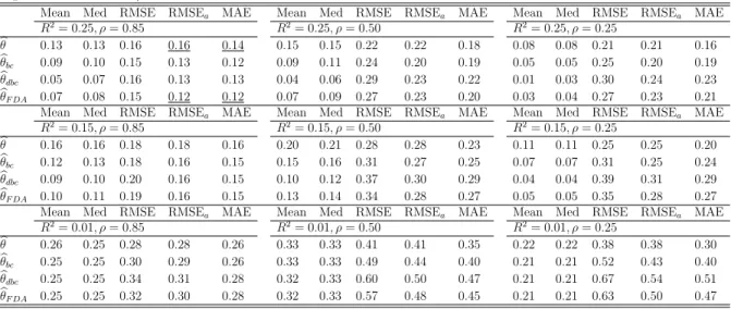
Tables I-III report the summary statistics of the empirical distributions of the instru-mental variable estimatorθb, the bootstrap bias corrected estimatorθbbc, the double bootstrap

bias corrected estimator θbdbc, and the bias corrected estimator using the fast approximation

b

θF DA. In particular, the columns show the sample mean, the sample median (Med), the

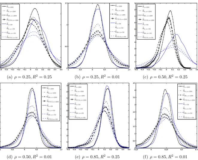
root mean square error RMSE, and the mean absolute error MAE. Figure 1 plots the kernel density estimates of the empirical distributions of the bootstrap estimators for selected DGP parametrization.

The results for the linear IV estimator θbare conventional. As the degree of overidenti-fication increases with the number od instruments moving from K = 5 to K = 10, there is an increase in the mean and median bias while the RMSE goes down. Increasing the sample size results in considerable decrease in the bias and increase in efficiency as can be seen when comparing Table II to Table III. If the instruments are strong (high R2), the presence of endogeneity is not a disaster even for high values ofρ. In Table I for example, the bias of θb

increased from 0.04 to 0.07 when ρ increased from 0.25 to 0.85

The statistical properties of the single bias corrected estimator θbbc and the double

boot-strap bias corrected estimatorθbdbc in tables I-III follow existing predictions in the literature.

For all the DGP configurations with R2 _{∈ {}₀_.₁₅_,₀_.₂₅_}_{, the bias of} _θb

dbc is smaller than that

of bθbc which in turn is significantly reduced compared to θb. In Table II for R2 = 0.25 and

ρ = 0.85, the single bootstrap reduces the bias by 29% while the double bootstrap further reduces the gap by 59%. These percentage reductions are higher (41% and 85% respectively) when ρ = 0.25. However, reducing the bias may increase the variance, or even the mean squared error. Indeed, this is the case in most configurations except for the case ofR2 = 0.25 and ρ= 0.85 and K = 10 where the RMSE of bθ decreased by 3.8% for n = 50.

This result is not new. Hsu et al. (1986) find that the bias reduction from bootstrapping the two stage least squares is achieved at the expense if increased variance. MacKinnon and Smith (1998) argue that reducing the bias may increase the variance and the root mean squared error of the bias corrected estimator depending on the shape of the bias function and on the variance of the initial estimator. We conjecture that the shape of the bias function of the IV estimator depends on the relevance of the instruments and the severity of the endogeneity problem. In addition, the increased variance may be due to few erratic bootstrap estimates θb∗_b and bθ∗∗_b,j. Following Hsu et al. (1986) and Shao (1990), we compute the adjusted root mean squared error RMSEa by deleting 2.5% from the top and 2.5% from

the bottom of the 5,000 bias corrected estimates. The results show no significant increase in the adjusted RMSE forθbbc. The mean bias of the double bootstrap estimator bθdbc is smaller

than that of the single bootstrap estimator θbbc. However, this gain in bias does not offset

the increased RMSE and RMSEa.

The proposed approximation of the double bootstrap bias produces estimators with higher bias reduction than the single bootstrap for all configurations. This reduction comes with lower variance than the double bootstrap corrected estimator. The proposed estimator

b

θF DA has lower mean absolute error MAE and RMSE than bθdbc. In addition to reduced bias,

this estimator has lower RMSEa and MAE than the IV estimatorθband the single bootstrap

(11)

The results are even more promising for the proposed approximation when the sample size is increased from n = 50 to n = 200. Table III shows that for models with relevant instruments, the proposed bias corrected estimator not only achieves a lower bias than the single bootstrap but also outperforms the double bootstrap corrected estimator. In Table III when _R2 _{= 0}_._{25 and} _ρ _{= 0}_._85, _θb

dbc reduces the bias of θbfrom 0.039 to −0.019 while θbF DA

further reduces the bias to 0.003.

Figure 1 provides an overview of the effect of instrument relevance and sample size on the sampling distributions of the alternative estimators. The plots show that in the presence of weak instruments (plots with _R2 = 0.01), the bias of all estimators is higher, the increase in the variance of the bootstrap bias corrected estimators is also higher. Increasing the sample size from n = 50 to n = 200 has little effect on both the bias and the variance unless the instruments are relevant and the endogeneity is moderate (see Figure 1(c)). In addition, the evidence from the Monte Carlo suggests that the bootstrap is less effective in reducing the finite sample bias when the instruments are weak.

6 Conclusion

The theory predicts that iterating the bootstrap principle increases the accuracy of the bootstrap. This increased accuracy comes at an enormous computational cost. This paper has presented a new computationally efficient technique for bias correction which removes the requirement to perform the computationally intensive inner loop of the double bootstrap. The proposed approximation converges to the theoretical bias adjustment of the double bootstrap. The new bootstrap bias corrected estimator is effective in reducing the bias of the single bootstrap and, in the example considered, is more precise than the double bootstrap. In the linear instrumental variable model, the bias function of the IV estimator depends on the instruments relevance, the degree of endogeneity and the number of instruments. We find that the bootstrap as a method to reduce the bias is less effective when the instruments are weak regardless of the sample size. In the case of weak identification, models with high degree of endogeneity have lower mean and median bias. This result warrants further investigation.

(12)

References

Beran, R. (1990) “Refining Bootstrap Simultaneous Confidence Sets,”Journal of Statistical Planning and Inference 43, 205–213.

Beran, R. (1988) “Prepivoting Test Statistics: a Bootstrap View of Asymptotic Refine-ments,” Journal of the American Statistical Association 83, 687–697.

Beran, R. (1987) “Prepivoting to Reduce Level Error in Confidence Sets,” Biometrika 74, 457–468.

Davidson, R. and J. G. MacKinnon (2007) “Improving the Reliability of Bootstrap Tests with the Fast Double Bootstrap,” Computational Statistics and Data Analysis 51 (7), 3259–3281.

Davidson, R. and J. G. MacKinnon (2002a) “Bootstrap J tests of Nonnested Linear Regres-sion Models,” Journal of Econometrics 109, 167–193.

Davidson, R. and J. G. MacKinnon (2002b) “Fast Double Bootstrap Tests of Nonnested Linear Regression Models,” Econometric Reviews 21, 417–427.

Davison, C., A and D. V. Hinkley (1997) “Bootstrap methods and their application,” In Cambridge Series on Statistical and Probabilistic Mathematics (Cambridge University Press).

Efron, B. (1987) “Better Bootstrap Confidence Intervals,” Journal od American Statistical Association 82, 171–200.

Efron, B. (1979) “Bootstrap Methods: Another Look at the Jackknife,”Annals of Statistics 7, 1–26.

Efron, B. and R. Tibshirani (1986) “Bootstrap Methods for Standard Errors, Confidence Intervals, and other Measures of Statistical Accuracy,” Statistical Science 1 (1), 54–77. Flores-Lagunes, A. (2007) “Finite Sample Evidence of IV Estimators under Weak

Instru-ments,” Journal of Applied Econometrics 22, 677–694.

Giacomini, R., D. N. Politis, and H. White (2007) “A warp-speed method for conducting Monte Carlo experiments involving bootstrap estimators,” Unpublished manuscript. Guggenberger, P. (2008) “Finite Sample Evidence Suggesting a Heavy Tail Problem of the

Genralized Method of Empirical Likelihood Estimator,” Econometric Reviews 26, 526– 541.

Hall, P. (1992) The Bootstrap and Edgeworth Expansion, New York: Springer-Verlag. Hall, P. (1986) “On the Bootstrap and Confidence Intervals,” The Annals of Statistics 14

(13)

Hall, P. and L. Horowitz, Joel (1996) “Bootstrap Critical Values for Tests Based on Gener-alized Method of Moments Estimators,” Econometrica 64, 891–916.

Hall, P. and M. A. Martin (1988) “On Bootstrap Resampling and Iteration,”Biometrika 75, 661–671.

Horowitz, J. L. (2001) The Bootstrap 5, Chap. 52, 3159–3228: Heckman, J.J. and Leamer, E.E. (eds), Elsevier Science. in Handbook of Econometrics.

Hsu, Y. S., K. N. Lau, H. G. Fung, and E. F. Ulveling (1986) “Monte Carlo studies on the effectiveness of the Bootstrap bias reduction method on 2SLS estimates,” Economics Letters, 233–239.

Lee, S. M. S. and G. A. Young (1999) “The effect of Monte Carlo approximation on coverage error of double-bootstrap confidence intervals,” Journal of the Royal Statistical Society: Series B (Statistical Methodology) 61 (2), 353–366.

MacKinnon, J. G. and A. A. Smith (1998) “Approximate bias correction in econometrics,”

Journal of Econometrics (2), 205–230.

Shao, J. (1990) “Bootstrap estimation of the asymptotic variances of statistical functionals,”

Annals of the Institute of Statistics and Mathematics (4), 737–752.

Shi, S. G. (1992) “Accurate and Efficient Double-bootstrap Confidence Limit Method,”

Computational Statistics and Data Analysis, 21–32.

Appendix A: Proof of Corollary 1

We first establish convergence of R∗_n,B₁(x) to Eµ_bEµb

∗[R_n(X∗∗n, θ(µb_∗)) +x]: R∗_n,B₁(x) = B₁−1 B1 X b=1 Rn(X∗∗l,bn, θ(µb ∗ b)) +x (23)

Note that x depends only on the DGP _bµand therefore can be taken out of the conditional expectation. By the assumption of IID random draws,

E b µ∗R ∗ n,B1(x) =Eµb ∗{R_n(X∗∗n b , θ(bµ ∗ b))}+x,

and the variance

V b µ∗R ∗ n,B1(x) =B −1 1 Vµb ∗R_n(X∗∗n b , θ(µb ∗ b))→0, as B1 → ∞.

Applying the law of large numbers ,

B₁−1 B1 X l=1 Rn(X∗∗l,bn, θ(µb∗))→Ebµ ∗R_n(X∗∗_l,bn, θ(µb∗_b))≡E b µ∗R_n(X_b∗∗n, θ(µb∗_b)) (24)

(14)

as B1 → ∞. Similarly, using the law of large numbers and given that Eµb

∗R_n(X∗∗n

b , θ(µb

∗

b))

are IID random variables,

Eµ_bR ∗ n,B1(x) = EbµEµb ∗R ∗ n,B1(x) = B₁−1 B1 X b=1 E b µEµb ∗R_n(X∗∗n b , θ(bµ ∗ b)) +x = E b µEµb ∗[R_n(X∗∗n, θ(µb_∗)) +x].

In addition, given the IID assumption and

Vµ_bR ∗ n,B1(x) =B −1 1 VµbEµb ∗R_n(X∗∗n, θ(bµ∗))<∞,

therefore using the law of large numbers we establish,R∗_n,B

1(x)→EµbEbµ

∗R_n(X∗∗n, θ(µb∗)) +x

asB1 → ∞. Similar result can be established forRn,B1(x) by using the law of large numbers and the fact that the random variablesRn(X∗bn, θ(µbb)) are IID:

Rn,B1(x)→Eµb[Rn(X

∗n

, θ(µ_b∗)) +x], asB1 → ∞.

The fast approximation of the adjustment parameter γF DA satisfies γF DA = R

∗ n,B1(β(bµ)). Solving for γF DA, γF DA = 1 B1 B1 X b=1 (θ(µ_b∗∗_b )−θ(_bµ∗_b)) +β(µ_b) (25) = " θ(µ_b)− 1 B1 B1 X b=1 θ(µ_b∗_b) # + " 1 B1 B1 X b=1 (θ(µ_b∗∗_b )−θ(µ_b∗_b)) # (26) = " 1 B1 B1 X b=1 (θ(µ_b∗∗_b )−θ(µ_b∗_b)) # − " 1 B1 B1 X b=1 (θ(_bµ∗_b)−θ(µ_b)) # (27) = R∗_n,B 1(0)−Rn,B1(0) (28) → E b µEbµ ∗[R_n(X∗∗n, θ(bµ_∗))]−E b µ[Rn(X∗n, θ(µb∗))] (29) → γ(µ_b), as B1 → ∞. (30)

(15)

Table I: Monte Carlo results (10,000 replications; true θ= 0; number of instruments K = 5; sample size n = 50). Summary statistics for the distribution of alternative estimators of θ: the mean, the median (Med), root mean square error (RMSE), adjusted RMSE (RMSEa)

and the mean absolute deviation (MAE).

Mean Med RMSE RMSEa MAE Mean Med RMSE RMSEa MAE Mean Med RMSE RMSEa MAE

R2_{= 0}_.₂₅_{, ρ}_{= 0}_.₈₅ _R2_{= 0}_.₂₅_{, ρ}_{= 0}_.₅₀ _R2_{= 0}_.₂₅_{, ρ}_{= 0}_.₂₅ b θ 0.07 0.07 0.12 0.12 0.10 0.07 0.07 0.20 0.20 0.16 0.04 0.04 0.22 0.22 0.18 b θbc 0.026 0.043 0.14 0.11 0.11 0.02 0.04 0.23 0.19 0.18 0.00 0.02 0.27 0.21 0.20 b θdbc -0.02 0.01 0.18 0.13 0.12 -0.03 -0.00 0.29 0.22 0.21 -0.02 -0.01 0.32 0.25 0.24 b θF DA 0.01 0.04 0.16 0.12 0.11 0.00 0.03 0.26 0.20 0.18 0.00 0.01 0.28 0.21 0.20

R2_{= 0}_.₁₅_{, ρ}_{= 0}_.₈₅ _R2_{= 0}_.₁₅_{, ρ}_{= 0}_.₅₀ _R2_{= 0}_.₁₅_{, ρ}_{= 0}_.₂₅ b θ 0.13 0.14 0.19 0.19 0.16 0.11 0.12 0.25 0.25 0.20 0.07 0.07 0.30 0.30 0.23 b θbc 0.09 0.11 0.23 0.18 0.17 0.05 0.07 0.31 0.24 0.23 0.03 0.04 0.41 0.29 0.28 b θdbc 0.04 0.08 0.29 0.20 0.20 -0.01 0.03 0.40 0.29 0.28 -0.01 0.02 0.52 0.35 0.34 b θF DA 0.06 0.09 0.28 0.19 0.19 0.02 0.06 0.36 0.26 0.25 0.02 0.04 0.48 0.37 0.31

R2_{= 0}_.₀₁_{, ρ}_{= 0}_.₈₅ _R2_{= 0}_.₀₁_{, ρ}_{= 0}_.₅₀ _R2_{= 0}_.₀₁_{, ρ}_{= 0}_.₂₅ b θ 0.25 0.25 0.30 0.30 0.26 0.33 0.33 0.50 0.50 0.40 0.23 0.23 0.55 0.55 0.42 b θbc 0.24 0.24 0.37 0.31 0.30 0.32 0.32 0.69 0.54 0.51 0.23 0.23 0.84 0.63 0.60 b θdbc 0.24 0.24 0.46 0.36 0.34 0.32 0.31 0.92 0.66 0.64 0.24 0.23 1.14 0.82 0.79 b θF DA 0.24 0.24 0.44 0.34 0.33 0.32 0.32 0.87 0.62 0.60 0.24 0.23 1.07 0.76 0.73

Table II: Monte Carlo results (10,000 replications; trueθ = 0; number of instrumentsK = 10; sample size n= 50).

R2_{= 0}_.₂₅_{, ρ}_{= 0}_.₈₅ _R2_{= 0}_.₂₅_{, ρ}_{= 0}_.₅₀ _R2_{= 0}_.₂₅_{, ρ}_{= 0}_.₂₅ b θ 0.13 0.13 0.16 0.16 0.14 0.15 0.15 0.22 0.22 0.18 0.08 0.08 0.21 0.21 0.16 b θbc 0.09 0.10 0.15 0.13 0.12 0.09 0.11 0.24 0.20 0.19 0.05 0.05 0.25 0.20 0.19 b θdbc 0.05 0.07 0.16 0.13 0.13 0.04 0.06 0.29 0.23 0.22 0.01 0.03 0.30 0.24 0.23 b θF DA 0.07 0.08 0.15 0.12 0.12 0.07 0.09 0.27 0.23 0.20 0.03 0.04 0.27 0.23 0.21

R2_{= 0}_.₁₅_{, ρ}_{= 0}_.₈₅ _R2_{= 0}_.₁₅_{, ρ}_{= 0}_.₅₀ _R2_{= 0}_.₁₅_{, ρ}_{= 0}_.₂₅ b θ 0.16 0.16 0.18 0.18 0.16 0.20 0.21 0.28 0.28 0.23 0.11 0.11 0.25 0.25 0.20 b θbc 0.12 0.13 0.18 0.16 0.15 0.15 0.16 0.31 0.27 0.25 0.07 0.07 0.31 0.25 0.24 b θdbc 0.09 0.10 0.20 0.16 0.15 0.10 0.12 0.37 0.30 0.29 0.04 0.04 0.39 0.31 0.29 b θF DA 0.10 0.11 0.19 0.16 0.15 0.13 0.14 0.34 0.28 0.27 0.05 0.05 0.35 0.28 0.27

(16)

Table III: Monte Carlo results (10,000 replications; true θ = 0; number of instruments

K = 10; sample size n= 200).

R2_{= 0}_.₂₅_{, ρ}_{= 0}_.₈₅ _R2_{= 0}_.₂₅_{, ρ}_{= 0}_.₅₀ _R2_{= 0}_.₂₅_{, ρ}_{= 0}_.₂₅ b θIV 0.04 0.04 0.06 0.06 0.05 0.04 0.05 0.10 0.10 0.08 0.05 0.05 0.16 0.16 0.13 b θbc 0.01 0.02 0.06 0.05 0.05 0.01 0.02 0.11 0.09 0.08 0.02 0.03 0.18 0.15 0.14 b θdbc -0.02 -0.01 0.08 0.07 0.07 -0.02 -0.01 0.12 0.10 0.10 -0.01 0.00 0.22 0.18 0.17 b θF DA 0.00 0.01 0.07 0.06 0.05 0.00 0.01 0.11 0.09 0.09 0.01 0.02 0.20 0.16 0.15

Figure 1: Kernel density estimates of the empirical distribution of bootstrap biased corrected estimators of θ. Monte Carlo experiments: 10,000 replications; θ = 0; )K = 10; n =∈ {50,200}; ρ∈ {0.25,0.50,0.85}; R2 _{∈ {}₀_.₀₁_,₀_.₂₅_}_. −0.5 −0.4 −0.3 −0.2 −0.1 0 0.1 0.2 0.3 0.4 0.5 0 0.5 1 1.5 2 2.5 3 b θn=200 b θbc,n=200 b θdbc,n=200 b θF DA,n=200 b θn=50 b θbc,n=50 b θdbc,n=50 b θF DA,n=50 (a)ρ= 0.25, R2= 0.25 −1 −0.5 0 0.5 1 1.5 0 0.5 1 1.5 b θn=200 b θbc,n=200 b θdbc,n=200 b θF DA,n=200 b θn=50 b θbc,n=50 b θdbc,n=50 b θF DA,n=50 (b) ρ= 0.25, R2= 0.01 −0.5 −0.4 −0.3 −0.2 −0.1 0 0.1 0.2 0.3 0.4 0.5 0 1 2 3 4 5 5 0 1 2 3 b θn=200 b θbc,n=200 b θdbc,n=200 b θF DA,n=200 b θn=50 b θbc,n=50 b θdbc,n=50 b θF DA,n=50 (c) ρ= 0.50, R2= 0.25 −1 −0.5 0 0.5 1 1.5 0 0.5 1 1.5 2 2 0 0.5 1 1.5 2 b θn=200 b θbc,n=200 b θdbc,n=200 b θF DA,n=200 b θn=50 b θbc,n=50 b θdbc,n=50 b θF DA,n=50 (d) ρ= 0.50, R2_{= 0.01} −0.5 −0.4 −0.3 −0.2 −0.1 0 0.1 0.2 0.3 0.4 0.5 0 1 2 3 4 5 5 0 1 2 3 _b θn=200 b θbc,n=200 b θdbc,n=200 b θF DA,n=200 b θn=50 b θbc,n=50 b θdbc,n=50 b θF DA,n=50 (e) ρ= 0.85, R2_{= 0.25} −0.250 0 0.25 0.5 0.75 0.5 1 1.5 2 2.5 3 3.5 4 4.5 b θn=200 b θbc,n=200 b θdbc,n=200 b θF DA,n=200 b θn=50 b θbc,n=50 b θdbc,n=50 b θF DA,n=50 (f) ρ= 0.85, R2_{= 0.01}