Nonparametric Empirical Likelihood Density Functionals Estimation and Applications
By Ningning Wang Bachelor of Science Yantai Normal University
Yantai, CHINA 264300 July,2001
Master of Science
Huazhong University Science and Technology Wuhan, CHINA
43500 July,2004
Submitted to the Faculty of the Graduate College of the Oklahoma State University
in partial fulfillment of the requirements for
the Degree of
DOCTOR OF PHILOSOPHY December, 2013
Nonparametric Empirical Likelihood Density Functionals Estimation and Applications Dissertation Approved: Ibrahim Ahmad Thesis Adviser Joshua Habiger Lan Zhu Lisa A. Mantini
ABSTRACT
Name: Ningning Wang
Date of Degree: DECEMBER,2013
Title of Study: NONPARAMETRIC EMPIRICAL DENSITY FUNCTIONAL ESTIMATION AND APPLICATIONS
Major Field: STATISTICS
Chapter 2 of this dissertation presents a nonparametric empirical likelihood es-timation of kernel density functionals (ELKDFE), which are constructed based on a kernel density functional estimation (KDFE) and the concepts of empirical like-lihood. The work focuses on estimating the integration of square density function and a known function which has a derivative of order p, for p>0. In many applica-tions there may be extra information available to use, hence the concept of empirical likelihood becomes useful in providing a systematic approach for capturing the extra information. SoELKDFEreduces the MSE, especially when the sample size is small to moderate, and the difference of MSE between those two estimates decreases as the sample size increases.
Secondly, in Chapters 3 and 4, two new kernel estimators are proposed, GCA and LCA, and their rationales, properties, empirical likelihood versions, data-driven bandwidth selection, and applications are given as well. The bandwidth of the new approach is much tighter, catching the density’s humps and valleys is more accurate. These estimates can be used for fixed and sequential sampling. The empirical likeli-hood (EL) versions of the GCA and LCA are provided and shown to have smaller AMISE than that of the non-EL estimation, and the difference of MISE tends to shrink as the sample size increases.
The GCAandLGA estimates are applied to regression using a local polynomial setting. It is shown that the regression estimators based on GCA and LGA have smaller bias and variance than standard kernel regression estimators.
An investigation of the properties of cumulative distribution function estimation based on GCA and LGA shows that the new estimators have smaller MSE and better performance than standard kernel CDFestimation.
ACKNOWLEDGMENTS
I would like to express my sincere gratitude to my advisor, Dr. Ahmad, for providing able guidance and encouragement as I completed the work presented here. I would also like to thank Dr. Zhu, Dr. Habiger, and Dr. Mantini for serving as members of my dissertation committee.
I would also thank my department for giving me opportunities to teach, study, and do research. I am also grateful to other faculty and staff members in our department, without whom completion of my thesis would not have been possible.
Special thanks goes to my parents for their encouragement and support through-out my academic life, and to my brother, Penghua Wang, for his love, care, and encouragement, which allowed me to remain focused on my research.
I appreciate and thank all of my friends and colleagues for providing good suggestions and fruitful discussions.
Ningning Wang
1
1Acknowledgments reflect the views of the author and are not endorsed by committee members
TABLE OF CONTENTS
Abstract iii
Acknowledgments iv
Table of Contents v
List of Figures viii
1 Introduction and Literature Review 1
1.1 Introduction . . . 1
1.2 Kernel Density Estimation . . . 3
1.2.1 Statistical Result of Kernel Density Estimation . . . 4
1.2.2 Bandwidth Selection . . . 5
1.2.3 Kernel Smoothing Applications: Regression andCDFEstimation 6 1.3 Empirical Likelihood . . . 7
1.3.1 EL for Univariate Mean . . . 9
1.3.2 Empirical Likelihood-Based Kernel Density Estimation(ELKDE) . . . 10
1.4 Analysis of the Error Criteria . . . 11
1.5 Proposed New Kernel Density Estimates . . . 13
2 Nonparametric Empirical Likelihood Estimation of Density Func-tional 15 2.1 Introduction of Density Functional Estimation . . . 15
2.2 Methodology . . . 16 v
2.3 Statistical Result . . . 17
2.4 Applications . . . 19
2.4.1 Location Parameter . . . 20
2.4.2 Scale Parameter . . . 24
2.5 Appendix: proof the Theorem 2.3.1 . . . 27
3 New Kernel Density Estimations and their Empirical Likelihood Version 41 3.1 Introduction of Kennel Density Estimation . . . 41
3.1.1 New Kernel Density Estimations . . . 42
3.1.2 First New kernel Density Estimation: Local Coefficient Adjustment(LCA) . . . 42
3.1.3 Second New Kernel Density Estimation: Global Coefficient Adjustment(GCA) . . . 43
3.2 New Kernel Density Estimation Properties . . . 43
3.2.1 Bias and Variance . . . 44
3.2.2 MSE and MISE . . . 44
3.2.3 Estimation of Density functionals . . . 45
3.3 Bandwidth Selection . . . 47
3.3.1 Unbiased Cross Validation Method . . . 50
3.3.2 Bias Cross Validation Method . . . 53
3.4 Empirical Likelihood Based on GCAand LCAEstimation . . . 54
3.4.1 Empirical Likelihood Based on GCA(ELGCA) . . . 54
3.4.2 Empirical Likelihood Based on LCA Estimation (ELLCA) . 55 3.4.3 Bias and Variance of ELGCA and ELLCA . . . 55
3.5 Simulation Study . . . 57
3.6 Appendix . . . 65
3.6.2 Proof Theorem 3.2.3 . . . 67
3.6.3 Proof Theorem 3.4.1 . . . 73
4 GCA and LGA Applications: Regression and CDF Estimation 82 4.1 Introduction . . . 82
4.2 Random Design Regression Model . . . 82
4.2.1 Local Polynomial Based onGCA Estimators . . . 83
4.2.2 Local polynomial based onLCA Estimator . . . 88
4.2.3 Simulation Study . . . 93
4.3 Cumulative Distribution Function Estimation . . . 95
4.3.1 Properties . . . 96 4.3.2 Simulation Study . . . 97 4.4 Appendix . . . 103 5 Future Research 107 List of References 109 vii
LIST OF FIGURES
1 MSE of ˆµ from different distributions and sample size . . . 22 2 Estimated ˆµ from different distributions and sample sizes. Red line is
the ELKDFE; blue line is the KDFE; horizontal green line is µ= 2; vertical green line is optimal bandwidth based on equation (2.11) . . 23 3 MSE of ˆσ from different distributions and sample size . . . 25 4 Estimated ˆσ from different distributions and sample size. Red line is
the ELKDFE; blue line is the KDFE; horizontal green line is σ = 1; vertical green line is optimal bandwidth based on equation (2.11). . 26 5 Density estimate byGCAfrom bimodal distribution 0.5N(−1,4/9) +
0.5N(1,4/9) for different bandwidths . . . 48 6 Density estimate byLCA from bimodal distribution 0.5N(−1,4/9) +
0.5N(1,4/9) for different bandwidth . . . 49 7 Kernel estimates from standard normal distribution for sample size n=15 59 8 Density estimate from normal distribution for different sample size . . 60 9 Kernel density estimation from 0.75N(0,1)+0.25N(1.5,4/9) for sample
size n=15 . . . 61 10 Kernel density estimation from 0.75N(0,1) + 0.25N(1.5,4/9) for
dif-ferent sample size . . . 62 11 Kernel estimations from 0.5N(−1,4/9) + 0.5N(1,4/9) for sample size
n=15 . . . 63 12 Density estimate from normal distribution for different sample size . . 64 13 Estimated regression function with sample size n=50 . . . 94 14 Estimated regression function with sample size n=100 . . . 95 15 CDF estimation from normal distribution for sample size n=15 . . . . 98
16 CDF estimation from normal distribution for different sample sizes . 99 17 CDF estimation from 0.5N(−1,1) + 0.5N(1,1) for sample size n=15 . 100 18 CDF estimation from 0.5N(−1,1) + 0.5N(1,1) for different sample size 101 19 CDF estimation from 0.75N(0,1) + 0.25N(1.5,4/9) for sample size n=15102 20 CDF estimation from 0.75N(0,1) + 0.5N(1.5,4/9) for different sample
size . . . 103
1
Introduction and Literature Review
1.1 IntroductionNonparametric density estimation has been widely used with an array of new tools for statistical analysis. The main advantage of this approach is that it allows the exploration of large amounts of data without making specific distributional as-sumptions. This approach is in contrast to parametric estimation, in which it is assumed that the density comes from a given family, and the parameters are esti-mated by various statistical methods. Nonparametric density estimation is currently found in many fields, such as economics, signal processing, and image processing and reconstruction. Early contributors to the theory of nonparametric estimation include Rosenblatt (1956) and Parzen (1962), and their methods are still the most commonly used approach up to today. Comprehensive descriptions of various approaches to nonparametric estimation have been provided by Silverman (1986), and Wand and Jones (1994) have depicted more recent developments. These researchers provide a though discussion of kernel estimation, including details about the assumptions of kernel weight, estimator properties such as bias and variance, and guidelines for choosing the smoothness parameter bandwidthh. Empirical likelihood based on ker-nel density estimation (ELKDE) was introduced by Chen (1997), who showed that ELKDE reducesMSE and variance.
Empirical likelihood was first introduced by Owen (1988, 1990) for constructing confidence regions or intervals. It has many useful properties: such as, automatic
determination of the shape of confidence regions given the observed data set and a non-parametric version of Wilks’s Theorem. For these reasons, empirical likeli-hood has found many applications, such as in smooth functions of means (DiCiccio et al., 1991), estimating equations (Qin and Lawless, 1994), non-parametric density and regression function estimation (Owen, 1988; Chen, 1996; Chen and Qin, 2000), quantile estimation (Chen and Hall, 1993), and empirical likelihood-based kernel es-timation (Chen, 1997). Other useful sources of discussion about empirical likelihood include Owen (2001) and Chen and Keilegom (2009). In general, empirical likeli-hood combines the reliability of non-parametric methods with the effectiveness of the likelihood approach. The regions are invariant under transformations and often be-have better than confidence regions based on asymptotic normality when the sample size is small, a characteristic we show prevailing in our research. Moreover, they are of natural shape and orientation since the regions are obtained by contouring a log likelihood ratio, and they often do not require the estimation of the variance, as the studentization is carried out internally via the optimization procedure. The empir-ical likelihood method is appealing not only in obtaining confidence regions, but in its unique attraction in parameter estimation and formulating goodness-of-fit tests. On the computational side, empirical likelihood involves maximizing non-parametric likelihood supported on the data subject to some constraints. Owen (1988) showed that empirical likelihood regions for mean (univariate and multivariate) are always convex, so there is a unique solution for pi, where pi is the probability weight of the
observed data.
The aim of this chapter is to review the most important aspects of kernel density estimation and empirical likelihood based on kernel methods. In the remainder of this chapter, an introduction of kernel density estimation is given in Section 1.2; Sta-tistical results for the standard kernel density estimate is in Section 1.2.1; Bandwidth selection of kernel density estimation is shown in Section 1.2.2; The kernel smoothing
applications: regression and cumulative distribution function CDF estimation are presented in Section 1.2.3; An empirical likelihood introduction and review are given in Section 1.3; Empirical likelihood for univariate mean in Section 1.3.1; Empirical likelihood-based kernel density estimation is given in Section1.3.2; Analysis of error criteria is given in Section 1.4; New kernel density estimators are proposed in Section 1.5.
1.2 Kernel Density Estimation
The kernel estimation method is an important method in non-parametric density and distribution functions fitting. Suppose X1, X2,· · · , Xn are a sample of
inde-pendently and identically distributed random variable from some distribution with unknown density f. We are interested in estimating f. The kernel density estimate is ˆ f(x, h) = 1 nh n X i=1 K x−Xi h , (1.1)
where K is called the kernel, a bounded symmetric function satisfying R K(µ)dµ= 1,R µK(µ)dµ= 0, and R µ2K(µ)dµ < ∞, and h is a positive number depending on n, usually called the bandwidth or window width and satisfies h → 0 and nh → ∞, as n → ∞. Using the notation, Kh(µ) = h−1K(µ/h), the kernel density estimator
(1.1) can be written as ˆ fh(x) = 1 n n X i=1 Kh(x−Xi). (1.2)
For further information, refer to Wand and Jones (1994), Silverman (1986) and Alez (2012).
1.2.1 Statistical Result of Kernel Density Estimation
In this section, some theoretical properties of the standard kernel density estimator are derived. The assumptions and conditions are defined as in the previous section. So for a fixed h Bias( ˆf(x)) =h 2 2 f 00(x)µ 2(K) +o(h2) (1.3) Var( ˆf(x)) = 1 nhR(K)f(x) +o( 1 nh), (1.4) where R(K) = R
K2(µ)dµ. From these two equations, we have
MSE( ˆf(x)) = 1 nhR(K)f(x) + h4 4f 00 (x)2µ22(K) +o(h4+ 1 nh). (1.5)
The trade-off between bias and variance is controlled by MSE, when h is decreasing , the Bias is decreasing but variance is increasing. So a small hleads to a small Bias but large variance yields under smooth, and vice verse. As has already been pointed out, the smoothness of the estimate depends on the smoothing parameter h, and a closed-form expression can be obtained from minimizing the mean integrated square error (MISE)(1.12). We have
MISE( ˆf) = 1 nhR(K) + h4 4 R(f 00 (x))µ22(K) +o(h4 + 1 nh). (1.6)
Then the optimal bandwidth is achieved by minimizing AMISE (1.6)
hopt = R(K) nµ2 2(K)R(f00) 1/5 .
Using this optimal bandwidth, we have
infh>0MISE( ˆf) = 5 4[µ 2 2(K)R 4 (K)R(f00)]1/5n−4/5. 4
1.2.2 Bandwidth Selection
It is crucially important to select an appropriate bandwidth for the standard kernel density estimator. Since the early work on kernel methods emphasized asymptotic results, now determining an optimal hhas been the main research focus up to today. AsAMISE contains the unknown functionR(f00), several ”plug-in” procedures were proposed by estimating R(f00) with R( ˆf00) (see Scott and Terrell, 1987; Park and Marron, 1992). An automatic method for determining the optimal bandwidth is cross-validation (CV) which was first introduced by Rudemo (1982) and Bowman (1984). Scott and Terrell (1987) introduced biased cross-validation, which is considered a hybrid of cross-validation and plug-in, replacing an unknown value in AMISE with a cross-validation kernel estimator ˜R(f00). The recent kernel contrast method of Ahmad and Ran (2004) can be used for MISE minimization as well, but it is not really data adaptive. Moreover this method performs particularly well for regression, but not as well for density estimation. For more information about these methods, see the most exhaustive form comparison papers, by Jones et al. (1996) and Devroye et al. (1997) or the recent review paper by Heidenreich et al. (2013).
Cross-Validation Bandwidth Selection
Here we briefly introduce unbiased least square cross-validation, the idea of which is to consider the expansion of ISE in the following way
ISE(h) = Z ˆ f(x)2dx−2 Z ˆ f(x)f(x)dx+ Z f2(x)dx
Note that the last term is not dependent on h, so that we only need to consider the first two terms. The idea for choosing bandwidth is picking the one that minimizes
L(h) = Z ˆ f(x)2dx−2 Z ˆ f(x)f(x)dx
Consider the estimator CV(h) = Z ˆ f(x)2dx−21 n ˆ f−i(Xi) where ˆ f−i(x) = 1 (n−1)h X j6=i K x−Xj h
It is shown that CV(h) is the unbiased estimator of MISE−R
f2(x)dx. So the data-driven optimal bandwidth is
hCV =arg minhCV(h)
Biased cross-validation considers the asymptotic MISE, and its main idea is to replace the unknown quantity R(f00) in equation (1.6) by cross-validation estimator
˜ R(f00) =R( ˆf00)− 1 nh5R(K 00 ) =n−2X i6=j (K00∗K00)(Xi−Xj).
Then the biased cross-validation estimator (BCV) is given as
BCV(h) = R(K) nh + h4 4 µ 2 2(K)(f 00 ).
So, the selected bandwidth ishBCV =argmin BCV(h).
1.2.3 Kernel Smoothing Applications: Regression and CDF Estimation In this section, we describe nonparametric regression and CDFestimation based on standard kernel density estimation. There is a vast literature on flexible methods
for estimating regression functions andCDF. The NW estimator proposed indepen-dently by Nadaraya (1964) and Watson (1964) is based on locally weighted averages. Another popular estimate is the integral kernel estimate proposed by Gasser and Miller (1979). An alternative method of smoothing, the locally weighted regression, appeared in the statistical literature by Stone (1977) and Cleveland (1979). This method is still widely used today. It estimates the regression function at a particular point by locally fittingpth degree polynomial to the data, via weighted least squares. The CDF estimation is obtained by integrating a kernel estimator of the density. There has recently been extensive work on the estimation by kernel method of prob-ability densities and their derivatives; for a reference, see Wertz (1978) and Li and Racine (2007).
1.3 Empirical Likelihood
Empirical likelihood is a non-parametric method of inference based on a data-driven likelihood function. It allows the data analyst to use likelihood methods with-out assuming that the data come from a known family of distributions. The likelihood method is known to be efficient. For example, likelihood ratio tests have some good power properties. These tests can be modified to construct short confidence intervals or small confidence regions of the parameters. The empirical likelihood method com-bines reliability of the non-parametric methods and the flexibility and effectiveness of the likelihood approach. Now we will introduce the empirical likelihood.
Definition LetX1, X2,· · · , Xnbe i.i.drandom variables with the distribution
func-tion F. The empirical cumulative distribution function (ECDF) of X1, X2,· · · , Xn
is Fn(x) = 1 n n X 1 1(Xi6x),
Definition Assuming X1, X2,· · · , Xn, are independent real random variable with
common cumulative distribution function (CDF)F, the non-parametric likelihood of CDF ofF is L(F) = n Y i=1 (F(Xi)−F(Xi−)), whereF(x) =P r(X 6x) andF(x−) =P r(X < x), soP r(X =x) =F(x)−F(x−). Then for a CDF F, the ratios of the non-parametric likelihood for hypothesis tests and confidence intervals are defined in the following way,
R(F) = L(F) L(Fn)
.
Like parametric likelihood, suppose that we are interested in a parameter θ = T(F) for some functional T of the distribution. This F is a member of a set F of distributions. Define the profile likelihood ratio function,
R(θ) =sup{R(F)|T(F) =θ, F ∈F}.
Empirical likelihood hypothesis tests reject H0 : T(F0) = θ0, when R(θ0) < r0 for some threshold value r0. Empirical likelihood confidence regions are of the form
{θ|R(θ)>r0},
where threshold r0 may be chosen using an empirical likelihood theorem (ELT) 1.3.1, a non-parametric analogue of Wilk’s Theorem.
Theorem 1.3.1 (ELT) Let X1, X2,· · · , Xn be independent random variables with
common distribution F0. Let µ0 =E(Xi), and suppose that0< V ar(Xi)<∞. Then
−2log(R(µ0)) converges in distribution to χ2(1) as n→ ∞.
First, the chi-squared limiting distribution is the same as the typically found for parametric likelihood models with one parameter, which is Wilk’s Theorem. Second, it does not assume thatXi0sare bounded random variables. It is only required to have a bounded variance, which constrains how fast the sample maximum and minimum can grow as n increases.
1.3.1 EL for Univariate Mean
To test whetherµ=µ0, we need to computeR(µ0) and choose threshold value r0 by Theorem 1.3.1. Then reject the valueµ0at theαlevel, when−2logR(µ0)> χ
2,1−α
(1) . Empirical likelihood determines the pi by maximizing the empirical likelihood ratio
function Qn i=1npi or Pn i=1log(npi) subject to Pn i=1pi(Xi −µ0) = 0, pi > 0, and Pn
i=1pi = 1. The objective function
Pn
i=1log(npi) is strictly concave on a convex set of weight vectors. So there exists a unique global maximum in the domain.
We may proceed using the Lagrange multiplier to find p0is. Write
G= n X i=1 log(npi)−nλ n X i=1 pi(Xi−µ0) +γ( n X i=1 pi−1)
Setting to zero the partial derivative of G with respect to pi gives
∂G ∂pi = 1 pi −nλ(Xi−µ0) +γ = 0. Therefore, pi = 1 n 1 1 +λ(Xi−µ0) . (1.7)
The value of λ can be found by numerical search method, (for example, Newton’s method or Brent’s method), based on the equation
1 n n X i=1 (Xi−µ0) 1 +λ(Xi−µ0) = 0.
1.3.2 Empirical Likelihood-Based Kernel Density Estimation(ELKDE) In some statistical applications, additional information about f is available: for exmaple, the mean or variance of a distribution is known. This additional information usually can be expressed as
EXgl(X) = 0 (l = 1,2,· · · , q). (1.8)
where gl(X) are some known real functions. ELKDE (Chen, 1997) uses empirical
likelihood in conjunction with the kernel method to provide a systematic approach for capturing the extra information. Suppose the extra information can be formulated as equation (1.8), then ELKDE can be constructed by replacing n−1 in equation (1.2) with the empirical likelihood pi under extra information (1.8). Specifically pi can be
determined by maximizing a multinomial Qn
1npi subject to
X
pi = 1 and
X
pigl(Xi) = 0 (l = 1,2,· · · , q).
Letλ1, λ2,· · ·, λq be Lagrange multipliers corresponding to theq constraints. Define
λ = (λ1, λ2,· · · , λq)T and g(Xi) = {g1(Xi), g2(Xi),· · · , gq(Xi)}. Then the weight pi
are pi =n−1 1 +λTg(Xi) −1 (i= 1,2,· · · , n), (1.9) 10
where λ is the solution of n X i=1 gl(Xi) 1 +λTg(Xi) = 0 (l = 1,2,· · · , q).
ELKDE is obtained by replacing n−1 in KDE (1.2) with the pi at equation (1.9) ,
so ˆ fel(x) = 1 h n X i=1 piKh(x−Xi) (1.10)
It is shown that ELKDE has smaller variance and MSE than those of KDE. This is reasonable becauseELKDEachieves a smaller variance by using unequal weights, which offers more flexibility than KDE using equal weight n−1. In this Chapter, the ELKDE method is applied to estimate density functional, and it is shown that ELKDE has better performance than that of KDE in theoretical and simulation results .
1.4 Analysis of the Error Criteria
There are many criteria to evaluate ˆf(t) as an estimator of f(t) , such as the bias, square error, and distance error.
1. Bias
Bias is the difference between an estimator’s expectation and the true value of the parameter being estimated.
Bias[f(x)] = E{fˆ(x)−f(x)}
2. Mean Squared Error (MSE) , Mean Integrated Square Error (MISE) and Integrated Squared Error (ISE)
the estimator and the true value of the parameter being estimated at a single point.
MSE[ ˆf(x)] = Enfˆ(x)−f(x)o 2
(1.11)
Mean integrated squared error is the expected value of the square of the differ-ence between the estimator and the true value of the parameter being estimated at whole real line.
MISE[ ˆf(x)] = E
Z n
ˆ
f(x)−f(x)o2dx (1.12)
Integrated squared error globally measures the distance between the estimator and the true value of the parameter being estimated.
ISE[ ˆf(x)] =
Z
{fˆ(x)−f(x)}2dx (1.13)
3. Mean Distance Error (MDE) and Mean Integrated Distance Error(MIDE) The mean distance of using ˆf(x) to estimatef(x) is given by
MDE[ ˆf(x)] = E|f(x)ˆ −f(x)|. The MIDE is MIDE[ ˆf(x)] = E Z |fˆ(x)−f(x)|dx. The MSDE is MSDE[ ˆf(x)] = E sup x |f(x)ˆ −f(x)|. 12
The Bias, ISE and MISE are discussed in this dissertation. For more details on the MDE, MIDE and MSDE see Devroye and Lugosi (1996, 2001), Ahmad (2002), and Ahmad and Ran (2004).
1.5 Proposed New Kernel Density Estimates
Standard kernel density estimation is still one of most active areas of research in nonparametric statistics. But there are drawbacks to this method, such as choice of smoothing parameter(s), and difficulty in catching humps and valleys. For example, if the small bandwidth h is chosen, then the average kernel weightK(x−Xi
h ) for some
fixed x is only based on relatively few observations, not for all observations. So the estimate pays too much attention to the local data and does not allow for variation across the sample. But if the bandwidth is too large, then the estimate is too smooth and cannot catch details such as humps and valleys.
In view of the flaws of standard kernel smoothing, two new kernel density estima-tors GCAandLCA and their empirical likelihood versions are proposed in Chapter 3. Suppose the X1,· · · , Xn are independently and identically distributed from the
unknown distribution f, and these bandwidth of these two estimators is ih instead of h. So the bandwidth has two parts: one is the smoothing parameter h, and the other is the scale coefficient i. When choosing smaller h, for the fixed x, the value of K(x−Xi
h ) in standard kernel estimate is almost zero when Xi is far away from x.
In this situation, standard kernel density estimation is more ”wiggy”. But in the methods proposed in Chapter 3, the ratio of x−Xi
h divided by coefficient i, the value
of K(x−Xi
ih ) is not dependent on the distance between x and observation Xi, so the
average of K(x−Xi
ih ) at each pointxis dependent on the entire sample data instead of
just the local data (the data close to thex) in the standardKDE. These methods of choosing difference bandwidth do very well on balance between the local data and the whole sample data. Simulation study show that the new estimators can catch humps and valleys better that the standardKDE. The empirical likelihood version ofGCA
and LCA show that when the sample size is small to moderate, these methods are significantly better at catching humps and valleys than those of GCA and LCA. And when the sample size increases, the advantages shrink.
The applications of the proposed methods in the regression and CDFestimation of are developed in Chapter 4.
2
Nonparametric Empirical Likelihood Estimation of
Density Functional
2.1 Introduction of Density Functional Estimation
Immediately following the introduction of the kernel density estimation by Fix and Hodges (1951) and the study of its functional properties by Rosenblatt (1956), Parzen (1962),Watson and Leadbetter (1963) and Nadaraya (1964), many authors saw the potential of using a kernel density methodology to study inferential problems. The methodology was subsequently used in estimating regression (Nadaraya, 1964; Wat-son, 1964), testing goodness of fit (Bickel and Rosenblatt, 1973), testing independence (Rosenblatt, 1975; Ahmad and Li, 1997a), testing symmetry (Ahmad and Li, 1997b), and testing positive aging (Ahmad, 2000). Many books have been written on the subject. For univariate density estimation, more recent work has been conducted by Wand and Jones (1994), Bowman and Azzalini (1997), Simonoff (1996), Alez (2012) and Pons (2011), and in the multivariate case by Scott (1992) and Klemel¨a (2009). For econometric application, see Pagan and Ullah (1999), and Li and Racine (2007). Finally, for regression applications, see Hardle (1990).
Of particular interest to researchers is the subject of estimating density functionals of the type R γ(x)f(x)2dx =I(γ;f), where γ(x) is some known continuous function that has the pth derivative, for p > 0 . For γ(x) = 1 or x , Ahmad and Amezziane (2011) studied the basic kernel estimates properties of I(1;f) and I(x;f). These special cases are the location (I(x;f)) and scale (I(1;f)) parameters. Applications
of estimates of I(γ;f) are found in several areas. Among them many authors used variations of I(γ;f) and the estimates in evaluating the power of the nonparametric tests (Aubuchon and Hettmansperger, 1984) or obtaining estimates of the smoothing parameter (Sheather and Jones, 1991; Jones et al., 1991; Birge and Massart, 1995). 2.2 Methodology
In this work, I(γ, f) is estimated by the kernel density functional estimation (KDFE) as follows: ˆ I(γ;f) = 2 n(n−1)h X i<j γ(Xi) +γ(Xj) 2 K Xi−Xj h (2.1)
Moreover, in many applications there exists extra information which can be rep-resented by
E(gl(x)) = 0, l= 1,· · · , L, (2.2)
where gl(x) are some known real-valued functions. Using the concept of
empiri-cal likelihood (see Owen, 2001), in conjunction with the kernel method, provides a systematic approach for capturing the extra data information. The estimator (2.1) assigns an equal probability weight 1/(n(n+ 1)) to each data pair. However, if the extra data information is available as (2.2), then empirical likelihood based on kernel estimation is constructed by replacing 1/(n(n+ 1)) in (2.1) with empirical likelihood weightspipj, where p0is are the solution of the multinomial likelihood
Qn i=1pi subject to: n X i=1 pi = 1, n X i=1 pigl(Xi) = 0, l= 1,· · · , L. 16
Letλ= (λ1,· · · , λL)0 be the Lagrange multiplier and g(Xi) = (g1(Xi),· · · , gL(Xi))0. Then pi = 1 n{1 +λ 0 g(xi)}−1, i= 1,· · · , n, (2.3)
where λ is the solution to
n X i=1 gl(xi) 1 +λ0gl(xi) = 0, l= 1,· · · , L.
Hence, the empirical likelihood based on kernel density functional estimation (ELKDFE) of I(γ, f) is ˆ Iel(γ;f) = 1 h X i6=j pipj γ(Xi) +γ(Xj) 2 K Xi−Xj h , (2.4) where pi is given in (2.3). 2.3 Statistical Result
In order to study the mean squared error (MSE) and expectation of ELKDFEin comparison to those of the KDFE, we need the following customary conditions on K, h and f:
1. The density function f has pth continuous derivative, wherepis an integer and
p >1.
2. The kernel K(·) is a symmetric probability density with mean µk = 0 and
variance µ2(K) = σ2k <∞.
3. The sequence of constant {hn}, hn ≡ h is such that h → 0 and nh → ∞ as
In this section, the expectation and MSE of ELKDFE and KDFE are investi-gated, and it is shown that the Bias and the MSE of ELKDFE are both smaller than those of KDFE. The following is the main result.
Theorem 2.3.1
E( ˆIel) = E( ˆI)−
1 n
Z
gT(y)Σ−1g(y)γ(y)f2(y)dy+o(n−1), (2.5)
and MSE( ˆIel) = MSE( ˆI)− 2 n Z γ(y)f2(y)dy Z
gT(y)Σ−1g(y)γ(y)f2(y)dy+o(n−1), (2.6)
whereg(·)is the vector of extra information(eg, mean, variance·) andΣ =cov(gi, gj).
In addition,
E( ˆI) =
Z
γ(y)f2(y)dy+µ2(K)h2C1+o(h2) (2.7)
and MSE( ˆI) = 1 n2h Z γ2(y)f2(y)dy Z K2(µ)dµ+µ22(K)h4C12+ 4 nC2, (2.8) with C1 = 1 2 Z
γ(y)f00(y)f(y)dy+ 1 4
Z
γ00(y)f2(y)dy+1 2
Z
γ0(y)f0(y)f(y)dy (2.9)
and C2 = Z γ2(y)f3(y)dy− Z γ(y)f2(y)dy 2 , (2.10)
both assumed finite.
This theorem shows the difference of the expectation and MSE between ELKDFE and KDFE. Also, the difference of MSE between these two estimators is not de-pendent on the bandwidth h, so the optimal bandwidth for both methods can be obtained from equation (2.8). Thus it is given by
hopt =n−2/5 R γ2(y)f2(y)dyR K2(µ)dµ 4C1µ22(K) 1/5 . (2.11) 2.4 Applications
Define the location-scale family distributions as
f(x;µ, σ) = 1 σf0 x−µ σ , (2.12)
where f0 is bounded, and almost everywhere continuous probability density function (pdf). Consider the following functional,
I(x;f(·;µ, σ)) = Z xf2(x;µ, σ)dx = Z yσ+µ σ f02(y)dy =I(x;f0) + µ σI(1;f0). Which leads to µ=σI(x;f(·;µ, σ)) I(1;f0) −σI(x;f0) I(1;f0) , (2.13) and σ = I(1;f(·;µ, σ)) I(1;f0) . (2.14)
Thus estimating µ and σ is reduced to estimating I(γ;f), where γ(x) = x for µ and γ(x) = 1 for σ, provided the I(γ;f0) known. Suppose we wish to test H01 :
σ = σ0 or H02 : µ = µ0, then we have I(1;f(x, µ, σ)) = I(1;f0)σ under H01 or µ=c1I(x;f(x;µ, σ)) +c2 underH02, wherec1 =σ/I(1, f0) andc2 =−σII(1;(xf;f00)). Hence testing H01 or H02 is equivalent to testing H01∗ : I(1;f(x;µ, σ) = I(1;f0) or H02∗ : I(x;f(x;µ, σ) = I(x;f0) + µσ0I(1;f0) respectively. To test two or more samples H01: σ1 = · · ·= σk or H02 : µ1 = · · ·= µk, we only need to test H01 : I1(1;f1(x;µ, σ)) =
· · ·=Ik(1;fk(x;µ, σ)) orH02 :I1(x;f1(x;µ, σ)) = · · ·=Ik(x;f1(x;µ, σ)). Also notice
that I(γ;f0) is not required in those cases. In this work, by using extra information g, it shows that both the Bias and MSE of theELKDFEare distinctly smaller than those of the KDFE.
2.4.1 Location Parameter
By equation (2.13), estimating µ is reduced to I(x;f). If the extra information g is the location function g(y) =g0(y−µ), then Theorem 2.3.1 can be expressed as
follows:
Bias( ˆIel) = Bias( ˆI)−
µ n
Z
gT0(y)Σ−1g0(y)f02(y;µ)dy+o(h 2 ), (2.15) MSE( ˆIel) = MSE( ˆI)− 4 nµ 2 Z f02(y;µ)dy Z
g0T(y)Σ−1g0(y)dy+o(n−1), (2.16)
where
Bias( ˆI) = µh 2 2 µ2(K)
Z
f000(y;µ)f0(y;µ)dy+o(h2) (2.17)
Equation (2.16) shows that the empirical likelihood based on the kernel method has reduced the MSE, and this reduction decreases when sample size n increases.
Simulation
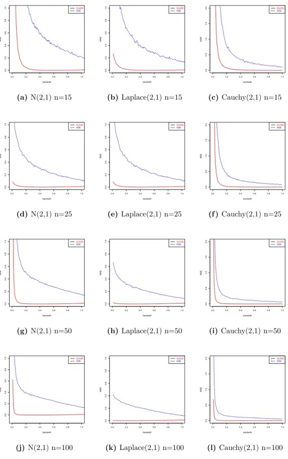
Generate the data from N(2,1), Laplace(2,1) and Cauchy(2,1) for the location parameter study with the sample sizes 50 and 100, with 1000 replications. Figure 1 shows that the MSE of the ELKDFE is smaller than that of the KDFE, and the
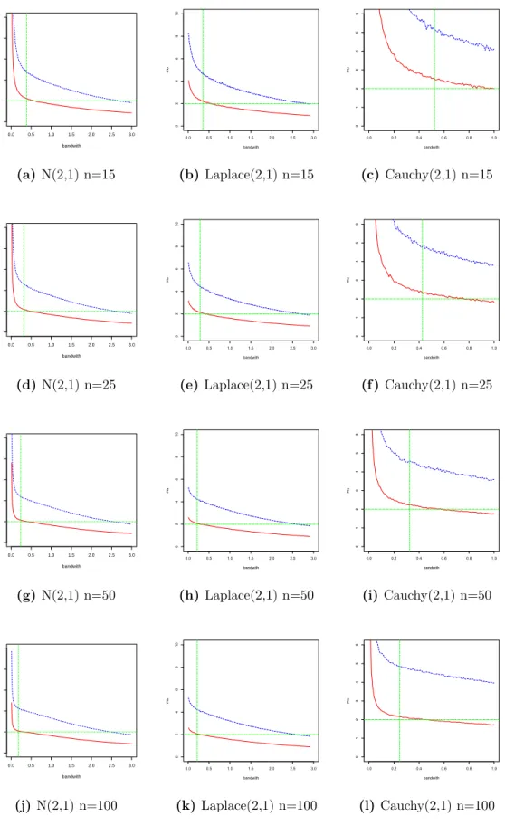
difference in MSE decreases as the sample size increases. ELKDFEperforms better for small and moderate sample sizes, and this advantage shrinks when the sample size becomes large. The MSE of ELKDFE is close to zero when h is increasing. When choosing the proper bandwidth h, MSE of ELKDFE is close to zero. Figure 2 shows that the ELKDFE is closer to the true value µ = 2 than that of KDFE. From these three cases, the ELKDFE not only reduces the MSE, but also provides bias correction with a proper bandwidth, which is shown in Theorem 2.3.1.
0.0 0.2 0.4 0.6 0.8 1.0 0.0 0.2 0.4 0.6 0.8 1.0 bandwith MSE ELKDE KDE (a)N(2,1) n=15 0.0 0.2 0.4 0.6 0.8 1.0 0.0 0.2 0.4 0.6 0.8 1.0 bandwith MSE ELKDE KDE (b) Laplace(2,1) n=15 0.0 0.2 0.4 0.6 0.8 1.0 0.0 0.5 1.0 1.5 2.0 bandwith MSE ELKDE KDE (c) Cauchy(2,1) n=15 0.0 0.2 0.4 0.6 0.8 1.0 0.0 0.2 0.4 0.6 0.8 1.0 bandwith MSE ELKDE KDE (d) N(2,1) n=25 0.0 0.2 0.4 0.6 0.8 1.0 0.0 0.2 0.4 0.6 0.8 1.0 bandwith MSE ELKDE KDE (e) Laplace(2,1) n=25 0.0 0.2 0.4 0.6 0.8 1.0 0.0 0.5 1.0 1.5 2.0 bandwith MSE ELKDE KDE (f ) Cauchy(2,1) n=25 0.0 0.2 0.4 0.6 0.8 1.0 0.0 0.2 0.4 0.6 0.8 1.0 bandwith MSE ELKDE KDE (g) N(2,1) n=50 0.0 0.2 0.4 0.6 0.8 1.0 0.0 0.2 0.4 0.6 0.8 1.0 bandwith MSE ELKDE KDE (h) Laplace(2,1) n=50 0.0 0.2 0.4 0.6 0.8 1.0 0.0 0.5 1.0 1.5 2.0 bandwith MSE ELKDE KDE (i) Cauchy(2,1) n=50 0.0 0.2 0.4 0.6 0.8 1.0 0.0 0.2 0.4 0.6 0.8 1.0 bandwith MSE ELKDE KDE (j)N(2,1) n=100 0.0 0.2 0.4 0.6 0.8 1.0 0.0 0.2 0.4 0.6 0.8 1.0 bandwith MSE ELKDE KDE (k) Laplace(2,1) n=100 0.0 0.2 0.4 0.6 0.8 1.0 0.0 0.5 1.0 1.5 2.0 bandwith MSE ELKDE KDE (l) Cauchy(2,1) n=100 Figure 1: MSE of ˆµfrom different distributions and sample size
0.0 0.5 1.0 1.5 2.0 2.5 3.0 0 2 4 6 8 10 bandwith m u (a)N(2,1) n=15 0.0 0.5 1.0 1.5 2.0 2.5 3.0 0 2 4 6 8 10 bandwith mu (b) Laplace(2,1) n=15 0.0 0.2 0.4 0.6 0.8 1.0 0 1 2 3 4 5 6 bandwith mu (c) Cauchy(2,1) n=15 0.0 0.5 1.0 1.5 2.0 2.5 3.0 0 2 4 6 8 10 bandwith m u (d) N(2,1) n=25 0.0 0.5 1.0 1.5 2.0 2.5 3.0 0 2 4 6 8 10 bandwith mu (e) Laplace(2,1) n=25 0.0 0.2 0.4 0.6 0.8 1.0 0 1 2 3 4 5 6 bandwith mu (f ) Cauchy(2,1) n=25 0.0 0.5 1.0 1.5 2.0 2.5 3.0 0 2 4 6 8 10 bandwith m u (g) N(2,1) n=50 0.0 0.5 1.0 1.5 2.0 2.5 3.0 0 2 4 6 8 10 bandwith mu (h) Laplace(2,1) n=50 0.0 0.2 0.4 0.6 0.8 1.0 0 1 2 3 4 5 6 bandwith mu (i) Cauchy(2,1) n=50 0.0 0.5 1.0 1.5 2.0 2.5 3.0 0 2 4 6 8 10 bandwith m u (j)N(2,1) n=100 0.0 0.5 1.0 1.5 2.0 2.5 3.0 0 2 4 6 8 10 bandwith mu (k) Laplace(2,1) n=100 0.0 0.2 0.4 0.6 0.8 1.0 0 1 2 3 4 5 6 bandwith mu (l) Cauchy(2,1) n=100 Figure 2: Estimated ˆµfrom different distributions and sample sizes. Red line is the ELKDFE; blue line is the KDFE; horizontal green line is µ= 2; vertical green
2.4.2 Scale Parameter
From equation (2.14), estimating scale parameter σ is equivalent to I(1;f). If extra informationg(x) is given, then Theorem 2.3.1 can be expressed as follows:
Bias( ˆIel) = Bias( ˆI)−
1 n
Z
gT(y)Σ−1g(y)f2(y;σ)dy+o(h2) (2.18) MSE( ˆIel) = MSE( ˆI)− 4 n Z f2(y;σ) Z
gT(y)Σ−1g(y)f2(y;σ)dy+o(n−1)
(2.19) where Bias( ˆI) = h 2 2 µ2(K) Z
f00(y;µ)f(y;µ)dy+o(h2), (2.20)
Equations (2.18) and (2.19) show that theELKDFEnot only reduces MSE but also reduces Bias. The difference decreases as the sample size n increases.
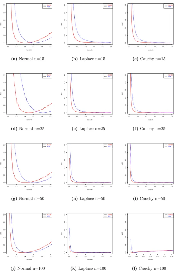
Simulation
Generate the data from N(0,1), Laplace(0,1) and Cauchy(0,1) for the scale parameter study with the sample sizes 15, 25, 50, and 100, with 1000 replications . Figure 3 shows that the ELKDFEhas a smaller MSE, and that difference decreases as the sample size increases. The ELKDFE works for small and moderate sample sizes, and this advantage shrinks when the sample sizes become large. The estimated difference decreases when the sample size increases, which is shown in Theorem 2.3.1.
0.0 0.2 0.4 0.6 0.8 1.0 0 20 40 60 80 100 bandwith MSE ELKDE KDE (a)Normal n=15 0.0 0.1 0.2 0.3 0.4 0.5 0.0 0.2 0.4 0.6 0.8 1.0 bandwith MSE ELKDE KDE (b)Laplace n=15 0.0 0.2 0.4 0.6 0.8 1.0 0.0 0.1 0.2 0.3 0.4 0.5 bandwith MSE ELKDE KDE (c)Cauchy n=15 0.0 0.2 0.4 0.6 0.8 1.0 0 20 40 60 80 100 bandwith MSE ELKDE KDE (d) Normal n=25 0.0 0.1 0.2 0.3 0.4 0.5 0.0 0.2 0.4 0.6 0.8 1.0 bandwith MSE ELKDE KDE (e) Laplace n=25 0.0 0.2 0.4 0.6 0.8 1.0 0.0 0.1 0.2 0.3 0.4 0.5 bandwith MSE ELKDE KDE (f ) Cauchy n=25 0.0 0.2 0.4 0.6 0.8 1.0 0 20 40 60 80 100 bandwith MSE ELKDE KDE (g)Normal n=50 0.0 0.1 0.2 0.3 0.4 0.5 0.0 0.2 0.4 0.6 0.8 1.0 bandwith MSE ELKDE KDE (h)Laplace n=50 0.0 0.2 0.4 0.6 0.8 1.0 0.0 0.1 0.2 0.3 0.4 0.5 bandwith MSE ELKDE KDE (i) Cauchy n=50 0.0 0.2 0.4 0.6 0.8 1.0 0 20 40 60 80 100 bandwith MSE ELKDE KDE (j)Normal n=100 0.0 0.1 0.2 0.3 0.4 0.5 0.0 0.2 0.4 0.6 0.8 1.0 bandwith MSE ELKDE KDE (k) Laplace n=100 0.00 0.05 0.10 0.15 0.20 0.25 0.30 0.0 0.2 0.4 0.6 0.8 1.0 bandwith MSE ELKDE KDE (l) Cauchy n=100 Figure 3: MSE of ˆσ from different distributions and sample size
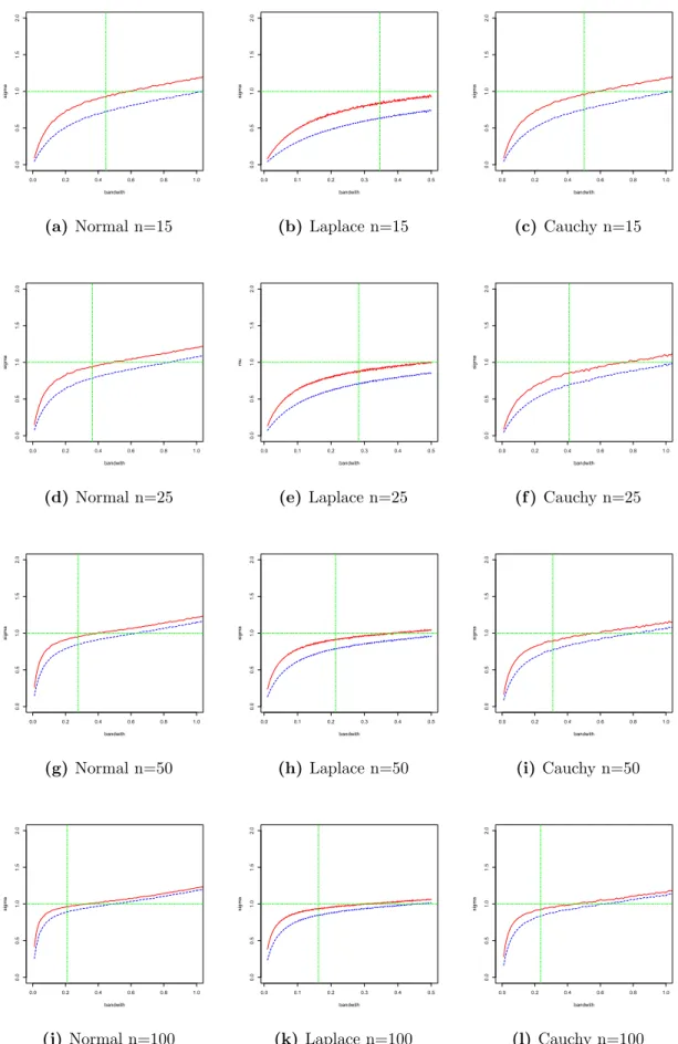
0.0 0.2 0.4 0.6 0.8 1.0 0.0 0.5 1.0 1.5 2.0 bandwith si gma (a)Normal n=15 0.0 0.1 0.2 0.3 0.4 0.5 0.0 0.5 1.0 1.5 2.0 bandwith si gma (b)Laplace n=15 0.0 0.2 0.4 0.6 0.8 1.0 0.0 0.5 1.0 1.5 2.0 bandwith si gma (c) Cauchy n=15 0.0 0.2 0.4 0.6 0.8 1.0 0.0 0.5 1.0 1.5 2.0 bandwith si gma (d) Normal n=25 0.0 0.1 0.2 0.3 0.4 0.5 0.0 0.5 1.0 1.5 2.0 bandwith mu (e) Laplace n=25 0.0 0.2 0.4 0.6 0.8 1.0 0.0 0.5 1.0 1.5 2.0 bandwith si gma (f ) Cauchy n=25 0.0 0.2 0.4 0.6 0.8 1.0 0.0 0.5 1.0 1.5 2.0 bandwith si gma (g)Normal n=50 0.0 0.1 0.2 0.3 0.4 0.5 0.0 0.5 1.0 1.5 2.0 bandwith si gma (h)Laplace n=50 0.0 0.2 0.4 0.6 0.8 1.0 0.0 0.5 1.0 1.5 2.0 bandwith si gma (i) Cauchy n=50 0.0 0.2 0.4 0.6 0.8 1.0 0.0 0.5 1.0 1.5 2.0 bandwith si gma (j)Normal n=100 0.0 0.1 0.2 0.3 0.4 0.5 0.0 0.5 1.0 1.5 2.0 bandwith si gma (k) Laplace n=100 0.0 0.2 0.4 0.6 0.8 1.0 0.0 0.5 1.0 1.5 2.0 bandwith si gma (l)Cauchy n=100
Figure 4: Estimated ˆσ from different distributions and sample size. Red line is the ELKDFE; blue line is theKDFE; horizontal green line isσ = 1; vertical green line
is optimal bandwidth based on equation (2.11). 26
2.5 Appendix: proof the Theorem 2.3.1
Proof Assume function γ(x) has pth derivative, γ(p)(x) 6= 0 and γ(p+i)(x) = 0 for i= 1,· · · , k. First show the equation (2.7) and (2.8).
E( ˆI) = 2 n(n−1)h X i<j E γ(Xi) +γ(Xj) 2 K Xi−Xj h = 2 n(n−1)h X i<j Z γ(x) +γ(y) 2 K x−y h f(x)f(y)dxdy = Z 1 h γ(x) +γ(y) 2 K(µ)f(x)f(y)dxdy = Z γ(y+µh) +γ(y) 2 K(µ)f(y+µh)f(y)dµdy = Z γ(y) +µhγ0(y) + (µh)2 2 γ 00(y) +γ(y) 2 ! K(µ)f(y+µh)f(y)dµdy = Z γ(y) + µh 2 γ 0(y) + (µh 2 ) 2γ00(y) K(µ) {f(y) +µhf0(y) + (µh) 2 2 f 00 (y)}f(y)dµdy = Z γ(y)f2(y)dy+µ2(K)h 2 2 Z γ(y)f00(y)f(y)dy + µ2(K)h 2 4 Z γ00(y)f2(y)dy+µ2(K)h 2 2 Z
γ(y)f0(y)f(y)dy+o(h2). (2.21) Now we will work on the Var( ˆI). It is not difficult to show that
Var( ˆI) = Var 1 n(n−1)h X i6=j γ(Xi) +γ(Xj) 2 K Xi −Xj h = 1 n2(n−1)2Var{ X i6=j γ(Xi) +γ(Xj) 2h K Xi−Xj h } = 2 n(n−1)Var{ γ(X1) +γ(X2) 2h K X1−X2 h } + 4(n−2) n(n−1)Cov{ γ(X1) +γ(X2) 2h K X1−X2 h , γ(X2) +γ(X3) 2h K X2−X3 h } =I1+I2. E{ γ(X1) +γ(X2) 2h K X1−X2 h }2 = Z Z γ(x) +γ(y) 2h 2 K x−y h 2 f(x)f(y)dxdy = Z Z γ(y+µh) +γ(y) 2h 2 hK(µ)2f(y+µh)f(y)dµdy = 1 h Z Z γ(y) + µh 2 γ 0 (y) + (µh 2 ) 2 γ00(y) 2 K(µ)2 {f(y) +µhf0(y) + (µh) 2 2 f 00 (y)}f(y)dµdy = 1 h Z γ2(y)f2(y)dy Z K2(µ)dµ +h Z K2(µ)µ2dµC1+o(h), where C1 = 14 R γ00(y)f2(y)dy+ 1 2γ
2(y)f00(y)f(y)dy+R
γ(y)γ0(y)f0(y)f(y)dy.
Then I1 = 2 n(n−1)E{ γ(X1) +γ(X2) 2h K X1−X2 h } − 2 n(n−1)[E{ γ(X1) +γ(X2) 2h K X1−X2 h }]2 = 2 n(n−1)h Z γ2(y)f2(y)dy Z K2(µ)dµ+ 2C1 n(n−1) Z K2(µ)µ2dµ − 2 n(n−1){ Z γ(y)f2(y)dy+µ2(K)h 2 2 Z γ(y)f00(y)f(y)dy+ µ2(K)h2 4 Z γ00(y)f2(y)dy+µ2(K)h 2 2 Z
γ(y)f0(y)f(y)dy}2+o(h2) = 2 n2h Z γ2(y)f2(y)dy Z K2(µ)dµ+o(n−2),
and E{ γ(X1) +γ(X2) 2h K X1−X2 h γ(X2) +γ(X3) 2h K X2−X3 h } = Z Z Z γ(x) +γ(y) 2h γ(y) +γ(z) 2h K x−y h K y−z h f(x)f(y)f(z)dxdydz = Z Z Z γ(y+µh) +γ(y) 2 γ(y) +γ(y−νh) 2
K(µ)K(ν)f(y+µh)f(y)f(y−νh)dµdydν = Z Z Z γ(y+µh) +γ(y) 2 γ(y) +γ(y−νh) 2
K(µ)K(ν)f(y+µh)f(y)f(y−νh)dµdydν = Z Z Z γ(y) + µh 2 γ 0 (y) + (µh 2 ) 2 γ00(y) γ(y)− νh 2 γ 0 (y) + (νh 2 ) 2 γ00(y) K(µ)K(ν){f(y) +µhf0(y) + (µh) 2 2 f 00 (y)}
f(y){f(y)−νhf0(y) + (νh) 2 2 f 00 (y)}dµdydν = Z γ2(y)f3(y)dy+ µ2(K)h 2 2 Z γ00(y)γ(y)f2(y)dy +µ2(K)h2 Z
γ2(y)f00(y)f2(y)dy+o(h2).
So that we have n(n−1) 4(n−2)I2 =E{ γ(X1) +γ(X2) 2h K X1−X2 h γ(X2) +γ(X3) 2h K X2−X3 h } −E γ(X1) +γ(X2) 2h K X1−X2 h E γ(X2) +γ(X3) 2h K X2 −X3 h = Z γ2(y)f3(y)dy+ µ2(K)h 2 2 Z γ00(y)γ(y)f2(y)dy +µ2(K)h2 Z
γ2(y)f00(y)f2(y)dy+o(h2)
− { Z γ(y)f2(y)dy+ µ2(K)h 2 2 Z
γ(y)f00(y)f(y)dy+ µ2(K)h2 4 Z γ00(y)f2(y)dy+ µ2(K)h 2 2 Z γ(y)f0(y)f(y)dy}2 = Z γ2(y)f3(y)dy−[ Z
γ(y)f2(y)dy]2+O(h2).
Then we get that
Var( ˆI) = 1 n2h Z γ2(y)f2(y)dy Z K2(µ)dµ+4C2 n +o(n −1 ), (2.22) where C2 = R γ2(y)f3(y)dy−[R γ(y)f2(y)dy]2. Now,
MSE( ˆI) =(Bias ˆI)2+ Var( ˆI) =µ22(K)h4(C1)2+ 1 n2h Z γ2(y)f2(y)dy Z K2(µ)dµ+ 4C2 n .
This gives us the optimal bandwidth h
hopt =n−2/5 R γ2(y)f2(y)dyR K2(µ)dµ 4C1µ22(K) 1/5 (2.23)
Next we show the equations (2.5) and (2.6). First, E( ˆIel) = E X i6=j pipj γ(Xi) +γ(Xj) 2h K Xi −Xj h . (2.24)
Plug in pi from equation (2.3), then
E( ˆIel) = E X 1≤i6=j≤n 1 n 1 1 +λTg(Xi) 1 n 1 1 +λTg(Xj) γ(Xi) +γ(Xj) 2h K Xi−Xj h = 1 n2 X 1≤i6=j≤n E 1 1 +λTg(Xi) 1 1 +λTg(Xj) γ(Xi) +γ(Xj) 2h K Xi−Xj h . 32
By using that λ=Op(n−1/2) and Taylor series expansion, then E 1 1 +λTg(Xi) 1 1 +λTg(Xj) γ(Xi) +γ(Xj) 2h K Xi−Xj h =E1−λTg(Xi) +λTg(Xi)gT(Xi)λ+op(n−1) 1−λTg(Xj) +λTg(Xj)gT(Xj)λ+op(n−1) γ(Xi) +γ(Xj) 2h K Xi−Xj h =E1−λTg(Xi) +λTg(Xi)gT(Xi)λ−λTg(Xj) +λTg(Xi)λTg(Xj) +λTg(Xj)gT(Xj)λ γ(Xi) +γ(Xj) 2h K Xi−Xj h =E γ(Xi) +γ(Xj) 2h K Xi−Xj h −EλT(g(Xi) +g(Xj)) γ(Xi) +γ(Xj) 2h K Xi−Xj h + EλTg(Xi)gT(Xi)λ+λTg(Xi)λTg(Xj) +λTg(Xj)gT(Xj)λ γ(Xi) +γ(Xj) 2h K Xi−Xj h . So, E( ˆIel) = 1 n2 X i6=j E{ γ(Xi) +γ(Xj) 2h K Xi−Xj h −EλT(g(Xi) +g(Xj)) γ(Xi) +γ(Xj) 2h K Xi−Xj h + E λTg(Xi)gT(Xi)λ+λTg(Xi)λTg(Xj) +λTg(Xj)gT(Xj)λ γ(Xi) +γ(Xj) 2h K Xi−Xj h } =E( ˆI)−E1+E21+E22+E23+o(n−1),
where E( ˆI) = 1 n2 X i6=j E γ(Xi) +γ(Xj) 2h K Xi−Xj h E1 = 1 n2 X i6=j EλT(g(Xi) +g(Xj)) γ(Xi) +γ(Xj) 2h K Xi−Xj h E21 = 1 n2 X i6=j EλTg(Xi)gT(Xi)λ γ(Xi) +γ(Xj) 2h K Xi−Xj h E22 =1 n2 X i6=j EλTg(Xi)λTg(Xj) γ(Xi) +γ(Xj) 2h K Xi−Xj h E23 = 1 n2 X i6=j EλTg(Xj)gT(Xj)λ γ(Xi) +γ(Xj) 2h K Xi−Xj h .
Now, we need to find E1,E21,E22 and E23, respectively. Using Taylor expansion for λ, we have following equation:
λ= Σ−11 n
X
g(Xi) +Op(n−1), (2.25)
where Σlm = Cov(gl(X), gm(X)), and µ2(K) =
R µ2K(µ)dµ. Plug in λ as in (2.25). Hence E1 = 1 n3 X i6=j,k E{Σ−1Xg(Xk)}T{g(Xi)+g(Xj)} γ(Xi) +γ(Xj) 2h K Xi−Xj h .
There are three cases to consider,k =i6=j,k =j =6 i and k 6=i6=j, then
E1 = n−1 n2 Eg T (Xi)Σ−1{g(Xi) +g(Xj)} γ(Xi) +γ(Xj) 2h K Xi−Xj h +n−1 n2 Eg T (Xj)Σ−1{g(Xi) +g(Xj)} γ(Xi) +γ(Xj) 2h K Xi−Xj h +(n−1)(n−2) n2 Eg T (Xk)Σ−1{g(Xi) +g(Xj)} γ(Xi) +γ(Xj) 2h K Xi−Xj h , 34
since X1,· · · , Xn are independent, and Egl(X) = 0, the third term is equal to zero, then E1 = 1 n Z Z g(x)TΣ−1{g(x) +g(y)} γ(x) +γ(y) 2h K x−y h f(x)f(y)dxdy +1 n Z Z gT(y)Σ−1{g(x) +g(y)} γ(x) +γ(y) 2h K x−y h f(x)f(y)dxdy+o(n−1) =1 n Z Z gT(y+µh)Σ−1{g(y+hµ) +g(y)} γ(y) + µh 2 γ 0 (y) + (µh 2 ) 2γ00 (y) K(µ)f(y+µh)f(y)dµdy +1 n Z Z
gT(y)Σ−1{g(y+µh) +g(y)}
γ(y) + µh 2 γ 0 (y) + (µh 2 ) 2γ00 (y) K(µ)f(y+µh)f(y)dµdy =1 n Z Z g(y) +µhg0(y) + µ 2h2 2 g 00 (y) T Σ−1 g(y) +µhg0(y) + µ 2h2 2 g 00
(y) +g(y) γ(y) + µh 2 γ 0 (y) + (µh 2 ) 2γ00 (y) K(µ) f(y) +µhf0(y) + h 2µ2 2 f 00 (y) f(y)dµdy + 1 n Z Z gT(y)Σ−1 g(y) +hµg0(y) + µ 2h2 2 g 00 (y) +g(y) γ(y) + µh 2 γ 0 (y) + (µh 2 ) 2 γ00(y) K(µ) f(y)−µhf0(y) + h 2µ2 2 f 00 (y) f(y)dµdy =4 n Z
Next, E21= 1 n2 X i6=j EλTg(Xi)gT(Xi)λ γ(Xi) +γ(Xj) 2h K Xi−Xj h = 1 n4 X i6=j,k,l E(Σ−1g(Xk))Tg(Xi)gT(Xi)Σ−1g(Xl) γ(Xi) +γ(Xj) 2h K Xi−Xj h .
There are three cases, k =l 6=i 6=j,k = l =i 6=j and k =l = j 6=i, also we know Eg(Xi) = 0, so the rest of cases are equal to zero. The second and third case are
order of n−2, so only the first case is considered.
E21= = 1 n4E n X l=k6=i6=j g(Xk)TΣ−1g(Xi)gT(Xi)Σ−1g(Xk) γ(Xi) +γ(Xj) 2h K Xi−Xj h +o(n−1) = (n−1)(n−2) n3 Eg(Xk) TΣ−1g(X i)gT(Xi)Σ−1g(Xk) γ(Xi) +γ(Xj) 2h K Xi−Xj h = 1 nEg T(X i)Σ−1g(Xk)g(Xk)TΣ−1g(Xi) γ(Xi) +γ(Xj) 2h K Xi−Xj h +o(n−1) = 1 nEg T(X i)Σ−1g(Xi) γ(Xi) +γ(Xj) 2h K Xi−Xj h +o(n−1) = 1 n Z Z gT(x)Σ−1g(x) γ(x) +γ(y) 2h K x−y h f(x)f(y)dxdy+o(n−1) = 1 n Z Z gT(x)Σ−1g(x) γ(x)− µh 2 γ 0 (x) + (µh) 2 ) 2γ00 (x) K(µ)f(x)f(x−µh)dxdµ+o(n−1) = 1 n Z gT(x)Σ−1g(x)γ(x)f2(x)dx+o(n−1). 36
Similarly, E23 =E22 = n1
R
gT(x)Σ−1g(x)γ(x)f2(x)dx+o(n−1). From above calcula-tions, then E( ˆIel)
E( ˆIel) =E( ˆI)−E1+E21+E22+E23+o(n−1) =E( ˆI)− 1
n
Z
gT(y)Σ−1g(y)γ(y)f2(y)dy+o(n−1),
where E( ˆI) is equation (2.21). Now, calculate E( ˆI2 el). E( ˆIel2) =EX i6=j pipj γ(Xi) +γ(Xj) 2h K Xi−Xj h X k6=l pkpl γ(Xk) +γ(Xl) 2h K Xk−Xl h = 1 n4E X i6=j X k6=l 1 [1 +λTg(X i)][1 +λTg(Xj)][1 +λTg(Xk)][1 +λTg(Xl)] γ(Xi) +γ(Xj) 2h K Xi−Xj h γ(Xk) +γ(Xl) 2h K Xk−Xl h .
Using Taylor expression, then E( ˆIel2) = 1 n4E X i,j X k,l [1−λTg(Xi) +λTg(Xi)gT(Xi)λ+o(n−1)] [1−λTg(Xj) +λTg(Xj)gT(Xj)λ+o(n−1)] [1−λTg(Xk) +λTg(Xk)gT(Xk)λ+o(n−1)] [1−λTg(Xl) +λTg(Xl)gT(Xl)λ+o(n−1)] γ(Xi) +γ(Xj) 2h K Xi−Xj h γ(Xk) +γ(Xl) 2h K Xk−Xl h = 1 n4E X i,j X k,l [1−λT(g(Xi) +g(Xj) +g(Xk) +g(Xl)) +λT(g(Xi)gT(Xj) +g(Xi)gT(Xk) +g(Xi)gT(Xl) +g(Xj)gT(Xk) +g(Xj)gT(Xl) +g(Xk)gT(Xl))λ] γ(Xi) +γ(Xj) 2h K Xi−Xj h γ(Xk) +γ(Xl) 2h K Xk−Xl h . 38
Simplifying can get E( ˆI12el) = E( ˆI12)−EλT(g(Xi) +g(Xj)) γ(Xi) +γ(Xj) 2h K Xi−Xj h γ(Xk) +γ(Xl) 2h K Xk−Xl h −EλT(g(Xk) +g(Xl)) γ(Xi) +γ(Xj) 2h K Xi−Xj h γ(Xk) +γ(Xl) 2h K Xk−Xl h +EλT(g(Xi)gT(Xj)λ γ(Xi) +γ(Xj) 2h K Xi−Xj h γ(Xk) +γ(Xl) 2h K Xk−Xl h +EλT(g(Xi)gT(Xk)λ γ(Xi) +γ(Xj) 2h K Xi−Xj h γ(Xk) +γ(Xl) 2h K Xk−Xl h +EλT(g(Xi)gT(Xl)λ γ(Xi) +γ(Xj) 2h K Xi−Xj h γ(Xk) +γ(Xl) 2h K Xk−Xl h +EλT(g(Xj)gT(Xk)λ γ(Xi) +γ(Xj) 2h K Xi−Xj h γ(Xk) +γ(Xl) 2h K Xk−Xl h +EλT(g(Xj)gT(Xl)λ γ(Xi) +γ(Xj) 2h K Xi−Xj h γ(Xk) +γ(Xl) 2h K Xk−Xl h +EλT(g(Xk)gT(Xl)λ γ(Xi) +γ(Xj) 2h K Xi−Xj h γ(Xk) +γ(Xl) 2h K Xk−Xl h
Hence,
Var( ˆIel) =E( ˆIel2)−(E ˆIel)2
=E( ˆI2)−2E1E( ˆI) + 2E( ˆI)E22+E1E1
−[E( ˆI)−E1+E21+E22+E23]2 =E( ˆI2)−2E1E( ˆI) + 2E( ˆI)E22+E1E1
−{[E( ˆI)]2+ (E1)2+ (E21+E22+E23)2−2E( ˆI)E1
−2E1(E21+E22+E23) + 2E( ˆI)(E21+E22+E23)}
=Var( ˆI)−2E( ˆI)(E21+E23)−(E21+E22+E23)2 + 2E1(E21+E22+E23) +o(n−1).
Finally, MSE( ˆIel) can be written as
MSE( ˆIel) = Var( ˆIel) + Bias( ˆIel)2
=Var( ˆI)−2E( ˆI)(E21+E23)−(E21+E22+E23)2
+ 2E1(E21+E22+E23) + (Bias( ˆI)−E1+E21+E22+E23)2+o(n−1) =MSE( ˆI) +E1E1−2Bias( ˆI)E1+ 2Bias( ˆI)(E21+E22+E23)
−2E( ˆI)(E21+E23) +o(n−1)
=MSE( ˆI) +E1E1−2Bias( ˆI)E1+ 2Bias( ˆI)(E21+E22+E23)
−2(Bias( ˆI) +I)(E21+E23) +o(n−1)
=MSE( ˆI) +E1E1−2Bias( ˆI)E1+ 2Bias( ˆI)E22−2(I)(E21+E23) +o(n−1) =MSE( ˆI)− 2
n
Z
γ(y)f2(y)dy
Z
gT(y)Σ−1g(y)γ(y)f2(y)dy+o(n−1).
3
New Kernel Density Estimations and their Empirical
Likelihood Version
3.1 Introduction of Kennel Density Estimation
The kernel method is a popular tool for the non-parametric estimation of the probability density function f. Suppose the independent and identical distribution sample X1,· · · , Xn from a continuous distribution, a kernel density estimator for f
at an arbitrary point x, is ˆ f(x) = 1 nh n X 1 K x−Xi h ,
whereKis a kernel function andhis a smoothing parameter that controls the smooth-ness of the fit. The choice of the shape of the kernel function is not a particularly important one. However, the choice of the value of the bandwidth is very important to trade off between the bias and the variance. When the bandwidth his increasing, the bias is increasing but the variance is decreasing. The estimate of point x is the average of 1hK(x−Xi
h ), and the kernel K is bounded. Also, in the symmetric density
function for small h, the estimate only pays attention to the local data (the observa-tions close to the point x) because the value ofK(x−Xi
h ) is almost equal to zero when
Xi is far away fromx. But for the largeh, the value ofK(x−hXi) is extremely close for
most observations, so in this case, it smooths away some details, such as humps and valleys. Based on these reasons, the kernel density estimation has some drawbacks,
such as difficulty in catching humps and valleys and finding the bandwidth. In this chapter, two new kernel density estimators are proposed in Section 3.1.1, and their empirical likelihood versions are also provided in Section 3.4.
3.1.1 New Kernel Density Estimations
Bandwidth plays an important role in the kernel density estimation. If bandwidth h is small, the estimate pays too much attention to the particular data set and does not allow for variation across the sample. If bandwidthh is large, the estimate is too smooth, in that it smooths away some details. To solve this problem, the bandwidthh of new estimations has two factors: one is the smoothing parameter hwhich controls smoothness, and the other is a scale coefficient which balances the local data and data from the whole sample. Under the same assumptions on the standard KDE, since the Xi is the random sample, for the sake of simplicity, choose the scale coefficient is
the index of Xi. So the bandwidth for X1 is h, X2 is 2h, and so on, Xn is nh. For
fixed x, the value of K(x−Xi
ih ) is not only dependent on the distance between x and
Xi, it is also dependent on the scale coefficient i. As a result, these estimators are
smooth enough and are also able to catch the humps and valleys. By minimizing the AM ISE, we reach the optimal hnew.opt = O(n−6/5), which is smaller than standard
kernel optimal bandwidth h=O(n−1/5). The new estimators therefore have smaller bandwidth ih; only thenth of the data X
n has the same order of the standard kernel
optimal bandwidth. Theoretical and simulation results show that the new kernel density estimators have better performance than that of standard KDE.
3.1.2 First New kernel Density Estimation: Local Coefficient Adjustment(LCA)
The first kernel estimator LCA is defined as follows:
ˆ fLCA(x) = 1 nh n X i=1 1 iK x−Xi ih . (3.1) 42
In this estimate, each kernel has adjusted coefficient 1/iand the bandwidth coefficient is i. Also R fˆLCA(x)dx = 1 when
R
K(µ)dµ= 1. So ˆfLCA(x) is the density function.
This estimate transforms ih∗ = h in the standard KDE. So this transformation makes the value of K(x−Xi
ih ) dependent not only on the distance of x and Xi. In this
way, by choosing a small h, this estimate is able to catch more details and is also sufficiently smooth, since the estimate pays attention to the whole sample data, not only some local data.
3.1.3 Second New Kernel Density Estimation: Global Coefficient Adjustment(GCA)
With the idea of LCA, choosing the same bandwidth, but this estimator has the global coefficient adjustment 2
n+1 instead of 1
i for eachK( x−Xi
ih ) inLCA. ThenGCA
is defined as follows: ˆ fGCA(x) = 2 n(n+ 1)h n X i=1 K x−Xi ih , (3.2)
and R fˆGCA(x)dx = 1 when
R
K(µ)dµ = 1 , so GCA is density function. Since the coefficient of this estimator is fixed, adding one more observation yields the following result, ˆ fGCA.n+1(x) = 2 (n+ 1)(n+ 2)h ( n X i=1 K x−Xi ih +K x−Xn+1 (n+ 1)h ) = n n+ 2 ˆ fGCA.n(x) + 2 (n+ 1)(n+ 2)hK x−Xn+1 (n+ 1)h .
Hence, ˆfGCA(x) is a recursive estimate that can be used in sampling schemes.
3.2 New Kernel Density Estimation Properties
In this section, four different measurement errors (see Section 1.4), are discussed for estimators GCAand LCA: bias, variance, MSE, and MISE.
3.2.1 Bias and Variance
Theorem 3.2.1 shows the bias and variance based on the GCAand LCA. Theorem 3.2.1 Bias[ ˆfGCA(x)] = 1 4n 2 h2µ2(K)f00(x) +o(n2h2), (3.3) Bias[ ˆfLCA(x)] = 1 6n 2h2µ 2(K)f00(x) +o(n2h2), (3.4) Var[ ˆfGCA(x)] = 2 n2hf(x)R(K) +o(n −1, h), (3.5) Var[ ˆfLCA(x)] = (Pn i=1 1 i) n2h f(x)R(K) +o(n −1 , h), (3.6) where µ2(K) = R µ2K(µ)dµ <∞, and R(K) =R K2(µ)dµ.
By minimizing AMISE, we can solve the new method optimal bandwidth hnew.opt =
O(n−6/5) for both estimators, while the standard KDE has the optimal bandwidth hopt =O(n−1/5).
3.2.2 MSE and MISE
Combine the Bias and the Var in Theorem 3.2.1, then MSE is given by the fol-lowing theorem. Theorem 3.2.2 MSE ˆfGCA(x) = 2 n2hR(K)f(x) + 1 16n 4h4µ2 2(K)(f 00 (x))2+o(n−1), (3.7) MSE ˆfLCA(x) = Pn i=1( 1 i) n2h R(K)f(x) + 1 36n 4h4µ2 2(K)(f 00 (x))2+o(n−1). (3.8) 44
This leads to the AMISE expression AMISEGCA = 2 n2hR(K) + 1 16n 4h4µ2 2(K)R(f 00 ), (3.9) and AMISELCA = Pn i=1( 1 i) n2h R(K) + 1 36n 4h4µ2 2(K)R(f 00 ). (3.10)
Then AMISE-optimal bandwidth is
hAM ISE.GCA=n−6/5 8R(K) µ2 2(K)R(f00) 1/5 , (3.11) and hAM ISE.LCA =n−6/5 9R(K)Pn i=1( 1 i) µ2 2(K)R(f00) 1/5 . (3.12)
Theorem 3.2.2 shows that optimal bandwidth h = o(n−6/5) for the GCA and h = o(n−6/5(Pn i=1 1 i) 1/5), whennis large,Pn i=1( 1
i)∼logn, so optimal bandwidth ofGCA
is larger than that of GCA. But the optimal bandwidths of GCA and LCA are both smaller than those of standard KDE.
3.2.3 Estimation of Density functionals
An important component of bandwidth selectors is the estimation of integrated squared density derivatives. The general integrated squared density derivative func-tional is
R(f(p)) =
Z
f(p)(x)2dx.
Under sufficient smoothness assumption on f, using integration by parts can get,
R(f(s)) = (−1)s
Z
Therefore, it is sufficient to study the functional estimation of this form
ψ =
Z
f(r)(x)f(x)dx,
for r even. Note that the sign of ψ2s is the same as that of (−1)s and ψr = 0 if r is
odd. Also note that
ψr = E{f(r)(x)}.
This motivates the density estimator
ˆ ψr(h) = Z f(r)(x)dFn(x) = n−1 n X i=1 ˆ f(r)(Xi;h). (3.13)
So for theGCA and LCA, we have
ˆ ψr(h)GCA = 2 n2(n+ 1)h n X i=1 n X j=1 1 jh r K(r) Xi−Xj jh = 2K (r)(0) n(n+ 1)hr+1 n X i=1 (1 j) r+ 2 n2(n+ 1)h n X i6=j ( 1 jh) rK(r) Xi−Xj jh , (3.14) ˆ ψr(h)LCA = 1 n2 n X i=1 n X j=1 1 jh r+1 K(r) Xi−Xj jh = K (r)(0) n2hr+1 n X i=1 (1 j) r+1+ 1 n2h n X i6=j ( 1 jh) r+1K(r) Xi−Xj jh , (3.15)
where h is the bandwidth and K is kernel density.
Theorem 3.2.3 E ˆψr(h)GCA = 2K(r)(0) n(n+ 1)hr+1 n X i=1 (1 j) r+ n−1 n ψr+ n2h2 4 µ2(K)ψr+2+o(n 2h2) E ˆψr(h)LCA = K(r)(0) n2hr+1 n X i=1 (1 j) r+1 +n−1 n ψr+ n2h2 6 µ2(K)ψr+2+o(n 2 h2) Var ˆψr(h)GCA = 3 n Z f(y)[f(r)(y)]2dy− 8 n[ Z f(y)f(r)(y)dy]2 Var ˆψr(h)LCA = 2 nh2r+1ψ0R(K (r)) + 4 n{ Z
f(y)[f(r)(y)]2dy]−ψr},
where ψr+s =
R
f(r)(x)f(s)(x)dx
From this theorem, we see that ˆψr(h) is an asymptotically unbiased estimator. Also
the variance of ˆψr(h) does not depend on h.
3.3 Bandwidth Selection
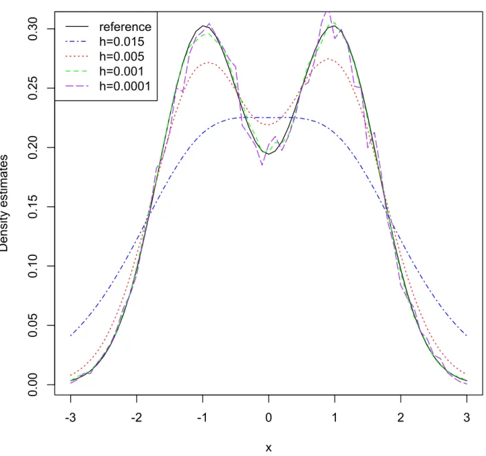
The choice of the bandwidth h is more important for the behavior of ˆf than the choice of kernel K. A small value of h makes the estimate look ”wiggly” and shows spurious features, whereas too large a value of h will lead to an estimate that is too smooth, in the sense that it is too biased and may not reveal structural features, such as bimodality. Figure 5 shows a mixture normal distribution 0.5N(−1,4/9) + 0.5N(1,4/9) by using GCAestimator for different values of h based on a sample of 100 observations for 1000 replications. And Figure 6 uses theLCAestimator. These two figures both show that for h = 0.001, the estimators are not smooth, but they still catch humps and valleys very well. Even if we choose a smaller bandwidth for each replication data set by choosing a random bandwidth ih instead of a fixed h, the estimates still allow for variation across samples. Unlike standard KDE, if we choose a smaller bandwidth, the estimate focuses on particular data and is overly noisy for most of the whole sampled data. In these two figures, a compromise is reached with h= 0.005 represented by the red dotted lines. These estimates are not
overly noisy and recover the essential structure of the true density. Whenh= 0.015, these estimates are overly smooth, since the bimodality structure has been smoothed away. -3 -2 -1 0 1 2 3 0.00 0.05 0.10 0.15 0.20 0.25 0.30 x D en si ty est ima te s reference h=0.015 h=0.005 h=0.001 h=0.0001
Figure 5: Density estimate by GCA from bimodal distribution 0.5N(−1,4/9) + 0.5N(1,4/9) for different bandwidths
-3 -2 -1 0 1 2 3 0.00 0.05 0.10 0.15 0.20 0.25 0.30 x D en si ty est ima te s reference h=0.015 h=0.005 h=0.001 h=0.0001
Figure 6: Density estimate by LCA from bimodal distribution 0.5N(−1,4/9) + 0.5N(1,4/9) for different bandwidth
In this section, the performance measures are mean integrated squared error MISE (1.12) and integrated squared error ISE (1.13). Based on these error cri-teria, we introduce a reliable data-driven estimator of the optimal bandwidth, the cross-validation via plug-in method which tries to minimize the MISE to findhopt.
3.3.1 Unbiased Cross Validation Method
The idea of unbiased cross-validation was introduced by Rudemo (1982) and Bow-man (1984). In this section, we employ this unbiased least squared cross-validation of bandwidth selection in the new kernel estimate GCA and LCA. We will begin our description of selection of bandwidth selectors. Ideally, for each sample, we would like to construct a density estimate to minimize the ISE (1.13). Least squares cross-validation attempts to address ISE rather than MISE. Its motivation comes from expanding the MISE of ˆf(.;h) to obtain
MISE ˆf(x;h) = E Z ( ˆf(x))2−2E Z ˆ f(x)f(x)dx+ Z f2(x)dx. (3.16)
Since the last term does not depend on h, minimizing the MISE ˆf(x, h) is equivalent to minimizing MISE ˆf(x, h)− Z f2(x)dx= E Z ( ˆf(x))2−2E Z ˆ f(x)f(x)dx. (3.17)
Then consider the cross-validation estimator
LSCV(h)≡ Z ˆ f(x)2dx−2 Z ˆ f−i(x)dFn(x) = Z ˆ f(x)2dx−2 n X i=1 ˆ f−i(Xi), (3.18) 50
where Fn(x) is empirical cumulative density function (ECDF) based on the sample with Xi deleted. ˆ f−i(x)GCA = 1 n(n−1)h{ i−1 X j=1 K x−Xj jh + n X j=i+1 K x−Xj (j−1)h } and ˆ f−i(x)LCA = 1 (n−1)h n X j=1 1 jK x−Xj jh
Now we check the expectations of LSCV(h)GCA and LSCV(h)LCA.
1 nE n X i=1 ˆ f−i(Xi)GCA = n X i=1 i−1 X j=1 1 n2(n−1)hK y−Xj jh f(y)dy+ n X i=1 n X j=i+1 1 n(n−1)hK y−Xj jh f(y)dy =E Z ˆ
f(y)GCAf(y)dy.
Same approach on LSCV(h)LCA,
1 nE n X i=1 ˆ f−i(Xi)LCA= E Z ˆ
f(y)LCAf(y)dy.
So,
E{LSCV(h)GCA}=MISE(h)GCA−R(f),
E{LSCV(h)LCA}=MISE(h)LCA−R(f).
Hence, for the fixed bandwidth, LSCV(h)GCA and LSCV(h)LCA are unbiased
Now we will introduce least squares unbiased cross-validation for the GCA. \ LSCVGCA(h) = Z ˆ f(x)2dx−2 Z ˆ f−i(x)dFn = n X i=1 n X j=1 Z 2 n(n+ 1)hK x−Xi ih 2 n(n+ 1)h − 4 n2(n−1)h n X i=1 { i−1 X j=1 K x−Xj jh + n X j=i+1 K x−Xj (j−1)h } = 2R(K) n(n+ 1)h + 4 n2(n+ 1)(n−1) X X i6=j Z 1 h2K x−Xi ih K x−Xj jh dx − 4 n2(n−1)h n X i=1 { i−1 X j=1 K x−Xj jh + n X j=i+1 K x−Xj (j−1)h } (3.19) = 2R(K) n2h + 4 n4 X X i6=j Z 1 h2K x−Xi ih K x−Xj jh dx − 4 n3h n X i=1 { i−1 X j=1 K x−Xj jh + n X j=i+1 K x−Xj (j−1)h }. (3.20)
The last equation replacesn±1 to n.
\ LSCVLCA(h) = Z ˆ f(x)2dx−2 Z ˆ f−i(x)dFn = n X i=1 n X j=1 Z 1 n2h2ijK x−Xi ih K x−Xj jh dx − 2 n(n−1)h X X i6=j 1 jK Xi−Xj jh = Pn i=1 1 iR(K) nh + 1 n2h2 X X i6=j Z 1 ijK x−Xi ih K x−Xj jh dx − 2 n(n−1)h X X i6=j 1 jK Xi−Xj jh (3.21) = Pn i=1 1 iR(K) nh + 1 n2h2 X X i6=j Z 1 ijK x−Xi ih K x−Xj jh dx − 2 n2h X X i6=j 1 jK Xi−Xj jh . (3.22)
3.3.2 Bias Cross Validation Method
The idea of biased least squares cross-validation methods for the classic KDE goes back to Scott and Terrell (1987). In this section, we employ this biased cross-validation method of bandwidth selection in the new kernel estimateGCAandLCA. The motivation comes from asymptotic expansion for AMISE as given in (3.9), and (3.10) contains only one unknown quantity ( R( ˆfGCA(p) ) and R( ˆfLCA(p) )) , where ˆfGCA
and ˆfLCA are new kernel estimators which are defined in section 3.1.1 and (p) is
the p derivatives. The BCVGCA and BCVLCA objective functions are obtained by
replacing the unknownR(f00) in the (3.9) and (3.10) by the estimators
] R(f00 GCA) = 4 n4h6 X i6=j Z (1 ji) 2K00 x−Xi ih K00 x−Xj jh dx, ] R(f00 LCA) = 1 n2h6 X i6=j Z (1 ji) 3K00 x−Xi ih K00 x−Xj jh dx.
These two selectors, R(f]00
GCA) and R(f]00LCA), used the data set of the i 6= j case.
These selectors use cross-validation techniques.
BCV(h)GCA = 2 n2hR(K) + n4 16h 4 µ22(K)R(f^00) GCA, (3.23) BCV(h)LCA = Pn i=1 1 i n2h R(K) + 1 9n 4h4µ2 2(K)R(f^00)LCA. (3.24)
3.4 Empirical Likelihood Based on GCA and LCA Estimation
In some statistical applications, additional information about f is available: the mean or variance of a distribution may be known, such as when estimating equations. This additional information usually can be expressed as (1.10).
3.4.1 Empirical Likelihood Based on GCA(ELGCA)
ELGCA uses empirical likelihood in conjunction with the new kernel method (GCA) to provide a systematic approach for capturing the extra information. Sup-pose the extra information can be formulated as equation (1.8), then,ELGCAcan be constructed by replacingn−1 in equation (3.2) with the empirical likelihood p
i under
extra information (1.8). Then pi can be determined by maximizing a multinational
Qn 1npi subject to X pi = 1, X ipi = n+ 1 2 and X pigl(Xi) = 0 (l= 1,2,· · · , q).
The second constraint makes the equation (3.26) to be density function. Let λ1, λ2,· · · , λq be Lagrange multipliers corresponding to the q constraints. Define
λ = (λ1, λ2,· · · , λq)T and g(Xi) = {g1(Xi), g2(Xi),· · · , gq(Xi)}. Then the weight pi
are pi =n−1 1 +λTg(Xi) −1 (i= 1,2,· · · , n), (3.25) 54
where λ is the solution of n X i=1 gl(Xi) 1 +λTg(Xi) = 0 (l = 1,2,· · · , q).
ELGCA is obtained by replacing n−1 with the pi (3.25) in (3.2), so
ˆ fel.GCA(x) = 2 (n+ 1)h n X i=1 piK x−Xi ih . (3.26)
It is easy to check that ˆfel.GCA(x) is a density function.
3.4.2 Empirical Likelihood Based on LCA Estimation (ELLCA)
This section, similar to Section 3.4.1, uses the empirical likelihood technique to apply the LGA estimation. Suppose the extra information about f is available and can be expressed as the 1.8. Thenpi can be determined by maximizing a multinational
Qn i=1npi X pi = 1, and X pigl(Xi) = 0 (l= 1,2,· · · , q).
ELLCA is obtained by replacing n−1 with the p
i at equation 1.9 in theLCA (3.1).
SoELLCA can be expressed
ˆ fel.LGA(x) = 1 h n X i=1 pi i K x−Xi ih . (3.27)
It easy to check ˆfel.LGA(x) is a density function.
3.4.3 Bias and Variance of ELGCA and ELLCA
In this section, the bias and variance of the new empirical likelihood-based kernel density estimators are investigated, and the performance of all estimators is compared. We assume the function gl and kernel K satisfied the following conditions:
1. for l= 1,· · · , q, gl are smooth functions with enough derivatives;
2. Egl(k)(X)<∞ for nonnegative integerk 64;
3. K is symmetric about zero and is the probability density. Theorem 3.4.1
E( ˆfel.GCA) =E( ˆfGCA) +o(n−1), (3.28)
E( ˆfel.LCA(x)) =E( ˆfLCA) +o(n−1), (3.29)
Var( ˆfel.GCA(x)) =Var( ˆfGCA(x))−
1 ng(x)
TΣ−1g(x)f(x)2+o(n−1), (3.30) Var( ˆfel.LCA(x)) =Var( ˆfLCA(x))−
1 ng(x)
TΣ−1g(x)f(x)2+o(n−1), (3.31)
where E ˆfGCA,E ˆfLCA,Var ˆfGCA and Var ˆfLCA are defined in Theorem 3.2.1.
Theorem 3.4.1 shows that the difference between E( ˆfel.GCA) and E( ˆfGCA) iso(n−1),
so is between E( ˆfel.GCA) and E( ˆfGCA). Also it is obvious that the coefficient of n−1
is always negative in the equation (3.30) and (3.31), there is an O(n−1) reduction in the variance of ˆfel.GCA(x) and ˆfGCA(x), so is variance of ˆfel.LCA(x) and ˆfLCA(x).
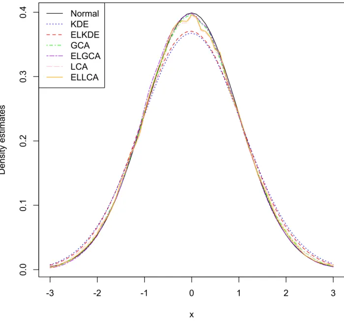
Using the empirical likelihood technique can reduce the variance with O(n−1), and this reduction decreases as the sample size increases. Simulations show that when n is greater than 25, ˆfel.GCA(x) and ˆfGCA(x) are almost the same for standard normal
distribution, and so are ˆfel.LCA(x) and ˆfLCA(x).
Immediately from the Theorem 3.4.1, the MISE for both estimators has the following results,
MISE ˆfel.GCA=MISE ˆfGCA−
1 n
Z
g(x)TΣ−1g(x)f(x)2dx+o(n−1) (3.32) MISE ˆfel.LCA =MISE ˆfLCA−
1 n
Z
g(x)TΣ−1g(x)f(x)2dx+o(n−1) (3.33)