2012
On nonparametric likelihood methods for weakly
and strongly dependent time series
Young Min Kim
Iowa State University
Follow this and additional works at:
https://lib.dr.iastate.edu/etd
Part of the
Economics Commons
,
Mathematics Commons
, and the
Statistics and Probability
Commons
This Dissertation is brought to you for free and open access by the Iowa State University Capstones, Theses and Dissertations at Iowa State University Digital Repository. It has been accepted for inclusion in Graduate Theses and Dissertations by an authorized administrator of Iowa State University Digital Repository. For more information, please [email protected].
Recommended Citation
Kim, Young Min, "On nonparametric likelihood methods for weakly and strongly dependent time series" (2012).Graduate Theses and Dissertations. 12365.
by
Young Min Kim
A dissertation submitted to the graduate faculty in partial fulfillment of the requirements for the degree of
DOCTOR OF PHILOSOPHY
Major: Statistics
Program of Study Committee: Daniel J. Nordman, Major Professor
Petrut¸a C. Caragea Heike Hofmann Mark S. Kaiser Stephen B. Vardeman
Iowa State University Ames, Iowa
2012
DEDICATION
I would like to dedicate this thesis to my parents Kim, Kwangwoong and Kang, Sooja and to my siblings Kim, Taeyoung and Kim, Jina whose support I would not have been able to complete this work. I would also like to thank my friends - Mr. and Mrs. Riddles, Eunice Kim, Jongho Im and other classmates at the Department of Statistics and Jihyoek Choi and Hyunsoo Kim for their loving guidance during the writing of this work. Also, I would like to thank our department staffs, Jeanette La Grange, Denise Riker, Sharon Shepard and Marlene Tjernagel.
TABLE OF CONTENTS
ACKNOWLEDGEMENTS . . . vi
CHAPTER 1. INTRODUCTION . . . 1
CHAPTER 2. A PROGRESSIVE BLOCK EMPIRICAL LIKELIHOOD METHOD FOR TIME SERIES . . . 5
2.1 Introduction . . . 6
2.2 Progression block empirical likelihood . . . 8
2.2.1 Description . . . 8
2.2.2 Main distributional results . . . 11
2.3 Numerical studies . . . 13
2.4 Data examples . . . 15
2.4.1 U.S. unemployment rates . . . 15
2.4.2 Records of hemispheric temperatures . . . 16
2.5 Conclusion remarks . . . 18
2.6 Proofs of main results . . . 19
2.6.1 Proof of Theorem1 . . . 21
2.6.2 Proof of Theorem2 . . . 22
CHAPTER 3. PROPERTIES OF A BLOCK BOOTSTRAP UNDER LONG-RANGE DEPENDENCE . . . 33
3.1 Introduction . . . 33
3.2 Block bootstrap distribution estimation under LRD . . . 35
3.2.1 Target processes . . . 35
3.3.1 Simulation design . . . 40
3.3.2 Summary of results . . . 42
3.4 Block bootstrap variance estimation under LRD . . . 44
3.4.1 Large-sample bias and variance properties . . . 45
3.4.2 Optimized block sizes and mean-squared error . . . 47
3.5 Concluding remarks . . . 50
3.6 Proofs of main results . . . 50
3.6.1 Proof of Theorem1 . . . 51
3.6.2 Proof of Theorem2. . . 53
CHAPTER 4. A FREQUENCY DOMAIN BOOTSTRAP FOR WHITTLE ESTIMATION UNDER LONG-RANGE DEPENDENCE . . . 65
4.1 Introduction . . . 66
4.2 Estimation Problem and Bootstrap Method . . . 69
4.2.1 Whittle estimation with linear time processes . . . 69
4.2.2 A frequency domain bootstrap method for Whittle estimation . . . 72
4.3 Main Distributional Results . . . 74
4.3.1 Assumptions . . . 74
4.3.2 Distributional results . . . 75
4.4 Simulation Studies . . . 77
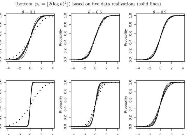
4.4.1 Properties of Whittle estimators . . . 78
4.4.2 Numerical studies of coverage accuracy in estimation . . . 83
4.5 Concluding Remarks . . . 96
4.6 Preliminary results and lemmas . . . 97
4.6.1 Preliminary results for proving Theorem1: Lemmas 1-7 . . . 98
4.6.2 Preliminary results for proving Theorem 2: Lemmas8-10 . . . 105
4.7 Proofs of main results . . . 115
4.7.1 Proof of Theorem1 . . . 115
CHAPTER 5. GENERAL CONCLUSIONS . . . 140
5.1 General Discussion . . . 140
ACKNOWLEDGEMENTS
I would like to take this opportunity to express my thanks to those who helped me with various aspects of conducting research and the writing of this thesis. First and foremost, Dr. Daniel J. Nordman for his guidance, patience and support throughout this research and the writing of this thesis. His insights and words of encouragement have often inspired me and renewed my hopes for completing my graduate education. I would also like to thank my committee members for their efforts and contributions to this work: Professors Petrut¸a C. Caragea, Heike Hofmann, Mark S. Kaiser and Stepehn B. Vardeman. I would additionally like to thank Dr. Kim and Dr. Lahiri for his guidance throughout the initial stages of my graduate career.
CHAPTER 1. INTRODUCTION
This dissertation investigates and develops three different nonparametric likelihood methods (e.g., resampling or empirical likelihood) for time series. For handling dependent data, current statistical methodology often relies on selecting parametric distributional models to accurately represent the data-generating process, which can be challenging. Additionally, inference drawn from a mistaken or misspecified probability model can potentially be misleading. Hence, the general advantage of nonparametric likelihood methods for time series is that these often allow valid statistical inference without stringent modeling assumptions about the underlying data distribution or exact dependence structure.
Specifically, the three nonparametric likelihood methods considered are Method 1: a blockwise empirical likelihood (EL),
Method 2: a block bootstrap,
Method 3: a frequency domain bootstrap.
Each method differs in form for building a nonparametric likelihood, but all methods involve “setting empirical probabilities” on observed data. EL creates a multinomial likelihood through a process of “probability profiling” data values. That is, probabilities are placed on data values, typically under a constraint involving expectations and estimating functions, and the product of these probabilities produces an EL function for inference (cf. Owen, 2001). In contrast, bootstrap methods resample data values, through an empirical probability distribution placed on these, in an effort to re-create pseudo versions of data (bootstrap data sets) which can be applied for inference (cf. Lahiri, 2003).
An important consideration in designing such methods for time series is appropriately ac-commodating the underlying (unknown and potentially complicated) time dependence
struc-original bootstrap for independent data fails under dependence. There are two general strate-gies for handling time dependence in resampling/EL methods (cf. Lahiri, 2003). One approach involves so-called “data blocking” whereby the original time series data are replaced by data blocks, consisting of consecutive groups of data points in time. Such data blocking helps to capture or preserve the dependence between neighboring temporal observations, and this ap-proach is used in methods 1 and 2 above. A different technique for treating the dependence structure in a resampling method is a data transformation. The goal of a data transformation is to weaken the dependence structure, without completely distorting it, whereby transformed observations can be handled as if these were (approximately) independent. This principle is applied in developing method 3.
An additional theme of this dissertation is the type or strength of the dependence in a stationary time process{Xt}. Ifr(k) = Cov(X0, Xk),k≥0, denote the process autocovariance
function, then we may generally classify the process as weakly or short-range dependent (SRD) if the covariances decay fast enough (i.e., r(k) → 0 as k → ∞) so that P∞
k=1|r(k)| < ∞
holds. In contrast, strongly or long-range dependent (LRD) processes are characterized by a slow covariance decay, r(k) ≈ Ck−α as k → ∞ for some C > 0 and 0 < α < 1, whereby
P∞
k=1r(k) = ∞ holds (cf. Beran, 1994). Processes exhibiting long-range dependence (LRD)
often have application, for example, in astronomy, hydrology and economics (cf. Beran, 1994; Montanari, 2003; Henry and Zaffaroni, 2003). The behavior of statistical methods can change dramatically between SRD and LRD cases, which complicates the development of appropriate resampling methods. For instance, Lahiri (1993) showed that the block bootstrap, which is generally valid under weak dependence (K¨unsch, 1989; Liu and Singh, 1993), is invalid for estimating the distribution of a sample mean from a class of long-memory processes.
The dissertation consists of three chapters (i.e., three manuscripts), one for each of the three methods listed above. We begin by considering weakly dependent processes and then transition to works involving LRD, where the approach to handling the time dependence in the methods also transitions as indicated in the following table.
Table 1.1 Main themes of each manuscript
Manuscript Method Methodological Approach Process Dependence Type
1 EL Data block-based SRD
2 Bootstrap Data block-based LRD, but including SRD
3 Bootstrap Data (Fourier) transformation LRD, but including SRD
weakly dependent time processes, called a progressive block empirical likelihood (PBEL). Unlike the standard BEL originally proposed by Kitamura (1997), the PBEL method doesnotrequire any block length selections. Because the performance of the standard BEL can depend critically on the block length choice, the PBEL method in contrast enjoys a type of robustness against block selection issues.
Manuscripts 2 and 3 consider different bootstrap problems for stationary, linear time series which could exhibit LRD. Manuscript 2 investigates the large-sample properties of a block bootstrap method for estimating the distribution of sample means. The results establish the validity of the block bootstrap under either LRD or SRD. Additionally, for estimating the variance of a sample mean under LRD, explicit expressions are provided for the large-sample bias and variance of block bootstrap estimators along with formulas for the theoretically optimal block sizes under LRD. Perhaps surprisingly, optimal blocks become shorter in length as the strength of the LRD increases.
Manuscript 3 develops a frequency domain bootstrap (FDB) method for a problem involv-ing Whittle estimation (Whittle, 1953), which is a popular technique for fittinvolv-ing parametric spectral density models to time series. For linear LRD time processes, the resulting Whittle es-timators are known to have normal limit laws. However, convergence to normality can be slow under LRD and the finite-sample distributions of Whittle estimators tend to be asymmetric. As a remedy, the FDB method can be used for calibrating confidence intervals in place of a normal approximation. Theoretical results establish the validity of the FDB for approximating the distribution of Whittle estimators for a broad class of time processes and spectral density models under LRD. The same results apply to SRD processes as well. Simulations show that the FDB method has better coverage accuracy than normal approximations under LRD.
References
Beran, J. (1994).Statistical methods for long memory processes. Chapman & Hall, London. Efron, B. (1979). Bootstrap methods: another look at the jackknife. Ann. Statist.,7, 1-26. Henry, M. and Zaffaroni, P. (2003). The long-range dependence paradigm for macroeconomics
and finance. In P.Doukhan, G. Oppenheim and M. S. Taqqu (eds.),Theory and Appli-cations of Long-range Dependence, pp. 417-438. Birkh¨auser, Boston.
Kitamura, Y. (1997). Empirical likelihood methods with weakly dependent processes. Ann. Statist.,25, 2084-2102.
K¨unsch, H. R. (1989). The jackknife and bootstrap for general stationary observations.Ann. Statist.,17, 1217-1261.
Lahiri, S. N. (1993). On the moving block bootstrap under long range dependence. Statist. Probab. Lett.,18,405-413.
Lahiri, S. N. (2003). Resampling methods for dependent data.Springer, New York.
Liu, R. Y. and Singh, K. (1992). Moving blocks jackknife and bootstrap capture weak de-pendence. In Exploring the Limits of Bootstrap, 225-248, R. LePage and L. Billard (editors). John Wiley &Sons, New York.
Montanari, A. (2003). Long-range dependence in hydrology. In P. Doukhan, G. Oppenheim and M. S. Taqqu (eds.),Theory and Applications of Long-range Dependence, pp. 461-472. Birkh¨auser, Boston.
Owen, A. B. (2001)Empirical likelihood. Chapman & Hall, London.
Singh, K. (1981). On the asymptotic accuracy of the Efron’s bootstrap.Ann. Statist.,9, 1187-1195.
CHAPTER 2. A PROGRESSIVE BLOCK EMPIRICAL LIKELIHOOD METHOD FOR TIME SERIES
A paper to be submitted to Journal of American Statistical Association
Young Min Kim, Soumendra N. Lahiri, Daniel J. Nordman
Abstract
This paper develops a new blockwise empirical likelihood (BEL) method for stationary, weakly dependent time processes, called the progressive block empirical likelihood (PBEL). In contrast to the standard version of BEL, which uses data blocks of constant length for a given sample size and whose performance can depend crucially on the block length selection, this new approach involves data blocking scheme where blocks increase in length by an arithmetic progression. Consequently, no block length selections are required for the PBEL method, which implies a certain type of robustness for this version of BEL. For inference of smooth functions of the process mean, theoretical results establish the chi-square limit of the log-likelihood ratio based on PBEL, which can be used to calibrate confidence regions. Simulation evidence indicates that the method can perform comparably to the standard BEL in coverage accuracy (when the latter uses a “good” block choice) and can exhibit more stability, all without the need to select a block length.
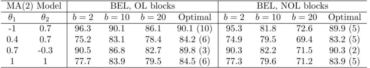
Empirical likelihood (EL) is a nonparametric methodology, introduced by Owen (1988, 1990), for producing likelihood-type inference without specification of a joint (parametric) distribution for the data. While EL for independent data has been studied in a variety of contexts (cf. Owen , 2001), our interest in this manuscript concerns EL for stationary, weakly dependent time series. In this setting, Kitamura (1997) first introduced the so-called blockwise empirical likelihood (BEL) method, which creates an EL ratio for inference by using data blocks (i.e., consecutive blocks of observations in time) to capture the underlying dependence structure. Such data-blocking has also played an important role in extending bootstrap and subsampling methods to time series, such as the moving block bootstrap of Hall (1985), K¨unsch (1989) and Liu and Singh (1992), and time subsampling methods of Carlstein (1986), Politis and Romano (1993), and Politis, Romano and Wolf (1999); see Lahiri (2003) for an overview of block resampling methods for time series. The BEL has been shown to apply for time series inference in a wide range of problems (cf. Lin and Zhang, 2001; Bravo, 2005, 2009; Zhang, 2006; Nordman, Sibbertsen and Lahiri, 2007; Chen and Wong, 2009; Nordman, 2009; Wu and Cao, 2011; Lei and Qin, 2011). Much like the moving block bootstrap, the standard implementation of BEL typically involves data blocks of constant length for an observed time series, and therefore requires a corresponding block length selection. However, the performance of BEL often depends critically on the choice of block length. As a small illustration, Table 2.1shows the effect of block length choice on the resulting BEL confidence intervals (CIs) for the mean of several MA(2) processes, based on a sample size n = 75 and either overlapping (OL) or non-overlapping (NOL) blocks. One observes that coverage accuracy can change intricately, depending on the block size b and underlying process, and that optimal block sizes may also vary by process and type of blocking scheme. Hence, the resulting CIs can lead to very different conclusions about the underlying mean parameter even when the block sizes do not differ by much (e.g., 5 or 10). The problem is compounded further by the fact that little is presently known about optimal block selection for the BEL method. As a result, the applicability of the BEL method in practice and the conclusions drawn from it are both subject to the variability
Table 2.1 Coverage percentages for 90% BEL CIs for the mean of processes
Xt = Zt + θ1Zt−1 + θ2Zt−2, (Zt iid standard normal), with n = 75 and
OL/NOL blocks of size b (from 4000 simulations). Coverage rates closest to nominal are indicated with associatedb in (·).
MA(2) Model BEL, OL blocks BEL, NOL blocks
θ1 θ2 b= 2 b= 10 b= 20 Optimal b= 2 b= 10 b= 20 Optimal
-1 0.7 96.3 90.1 86.1 90.1 (10) 95.3 81.8 72.6 89.9 (5)
0.4 0.7 75.2 83.1 78.4 84.2 (6) 74.9 79.5 69.4 83.2 (5)
0.7 -0.3 90.5 86.8 82.7 89.8 (3) 90.3 82.2 71.5 90.3 (2)
1 1 77.7 83.9 79.5 84.5 (6) 77.3 79.6 71.2 83.9 (5)
As a remedy, in this paper we propose aprogressiveblock empirical likelihood (PBEL) which uses an alternative data-blocking device and does not require a block length choice. Instead, for a given sample size, PBEL method uses data blocks which increase in length through an arithmetic progression. That is, in contrast to data blocks of constant length (for a given sample size) in the standard version of BEL, the resulting block sizes in the PBEL method are non-constant and are allowed to grow progressively larger until the given time sample is “used up.” More specifically, we define the empirical likelihood of a parameter by using successive (disjoint) blocks of observations of lengths 2,4, . . . ,2N such that these cover all of the given sample (upto a boundary block). As a consequence, given the sample size, the blocks in the construction of the PBEL are automatically well defined and it does not involve any block selection steps in the usual sense.
To investigate theoretical properties of the PBEL methodology, we consider the prototyp-ical problem of inference about the mean parameter and, more generally, inference about a parameter defined as a smooth function of the mean for a stationary, weakly dependent time series. We show that under suitable regularity conditions, a version of Wilks’ (1938) theorem holds in both the problems. Specifically, we show that like the traditional log-likelihood ratio statistic in a parametric inference problem with independent and identically distributed (iid) random variables, twice the negative log-EL ratio based on the PBEL method has a limiting chi-square distribution in each case, which can be used for calibrating confidence regions and
an explicit scale adjustment, depending on the choice of the fixed block length, to ensure a chi-square limit. In contrast, the blocking mechanism of the PBEL method automatically takes care of the scaling issue and does not require any explicit adjustments. Simulation evidence indicates that in finite samples, the PBEL can perform comparably to the standard version of BEL when the latter is used with a “good” choice of the block size. Consequently, the PBEL tends to work as well as the BEL at its optimal level, but can have a practical advantage in being robust to issues of block selection.
The rest of manuscript is organized as follows. In Section2.2, we describe the PBEL method and its associated data blocking scheme. The limiting distributional results are established to justify the method for confidence region estimation. In Section 2.3, we present a simulation study of the coverage accuracy of the PBEL method and provide some comparisons to the stan-dard BEL. Two real data examples are used to illustrate the PBEL methodology in Section2.4. Section2.5provides some concluding remarks and proofs of the main results are deferred to an Appendix (Section 2.6).
2.2 Progression block empirical likelihood
2.2.1 Description
Suppose we have an observed data stretchX1, . . . , Xn from a strictly stationary process {Xt: t∈Z}taking values inRd. To explain the PBEL method, we first consider problem of inference
on the process mean EXt=µ∈Rd. We return to inference on a wider class of “smooth model”
parameters in Section2.2.2.
For comparative purposes, it is initially helpful to recall the standard BEL formulation (Kitamura, 1997). This involves choosing an integer block length 1 ≤ b ≤ n and forming a collection of length b data blocks, which could possibly be maximally overlapping (OL) as given by {(Xi, . . . , Xi+b−1) : i= 1, . . . , K} withK =n−b+ 1, or non-overlapping (NOL) as
given by {(Xb(i−1)+1, . . . , Xib) :i= 1, . . . , K} with K =bn/bc. In either case, all blocks have
Bi,µ ≡Pbij=b(i−1)+1(Xj−µ) with NOL blocks) for defining a BEL function forµ given as LBEL,n(µ) = sup (K Y i=1 pi :pi ≥0, K X i=1 pi = 1, K X i=1 piBi,µ = 0d ) . (2.1)
and corresponding BEL ratio RBEL,n(µ) =Ln(µ)/K−K. The function LBEL,n(µ) quantifies the
plausibility of a value µ by maximizing a multinomial likelihood from probabilities {pi}Ki=1
assigned to the centered block sums Bi,µ under a zero-expectation linear constraint. Without
the mean constraint in (2.1), the multinomial product is maximized when each pi = 1/K
(i.e., the empirical distribution on blocks), leading to the ratio RBEL,n(µ). When 0d is in the
interior convex hull of {Bi,µ}Ki=1, then the expansion LBEL,n(µ) = QKi=1pi,µ > 0 holds with pi,µ =K−1(1 +λBEL,n,µBi,µ)
−1 ∈(0,1), i= 1, . . . , K, and a Lagrange multiplier λ
BEL,n,µ ∈Rd satisfying 0d= K X i=1 Bi,µ K(1 +λBEL,n,µBi,µ) ;
see Owen (1990) for more computational details with EL. Under certain mixing and moment conditions, and if the block size grows with the sample size n but at a smaller rate (i.e.,
b−1+b2/n→0 asn→ ∞), the log-EL ratio of the standard BEL has chi-square limit
−2 n
bK logRBEL,n(µ0) d
→χ2d, (2.2)
at the true mean parameter µ0. Aboven/(bK) represents a necessary block adjustment factor
for the distributional limit with BEL (cf. Kitamura, 1997). As mentioned in Section 2.1, not much is currently known about the best block lengthbselections for optimal coverage accuracy with BEL. In practice, one may typically borrow from the block bootstrap literature, where optimal orders for block sizes (across differing problems for distributional estimation) vary in powers of the sample size such as n1/3 or n1/4; see Hall, Horowitz and Jing (1995) and
Lahiri (2003, ch. 5) for more details on optimal block selections for time series block bootstrap methods.
We next present the PBEL method, which uses a collection of NOL data blocks given by
{(X(i−1)i+1, . . . , Xi(i+1)) :i= 1, . . . , N−1} ∪ {(X(N−1)N+1, . . . , Xn)}, andN denotes the
number N of blocks will be close to n, with the corresponding length of the largest block being approximately 2√n. While the last block could be dropped or defined in many ways without changing the asymptotic results, for a concrete rule, we let `1 = b √4n+ 1−1/2c
and`2=d
√
4n+ 1−1
/2eto defineN as`1 ifn−`1(`1+ 1)< `2(`2+ 1)−nand`2 otherwise;
this aims at a block number to closely divide the sample into a NOL blocks with a constant progression. To assess the likelihood of a given value ofµ, we then create centered block sums
Si,µ =Pmin
{i(i+1),n}
j=(i−1)i+1 (Xj−µ) and define a PBEL function Ln(µ) and ratio Rn(µ) as
Ln(µ) = sup (N Y i=1 pi :pi ≥0, N X i=1 pi = 1, N X i=1 piSi,µ = 0d ) , Rn(µ) = Ln(µ) N−N . (2.3)
The computation of Ln(µ) is the essentially same as for the standard BEL, where 0d in the
convex hull of {Si,µ}Ni=1 implies that Ln(µ) = QNi=1N−1(1 +λn,µSi,µ)−1 > 0 for a Lagrange
multiplierλn,µ∈Rd satisfying 0d= N X i=1 Si,µ N(1 +λn,µSi,µ) .
The next section establishes that, under mild dependence assumptions, the log-EL ratio from the PBEL method also has a chi-square limit, which can be used for tests or inverted to create confidence regions for EXt=µ.
We end this section with some qualifying remarks on the PBEL formulation. The PBEL again does not appeal to a particular block choice. The advantage of the PBEL is, generally, that this approach can perform comparably to the standard BEL when the later employs a good block selection and much better when the standard BEL employs a bad block choice; simulations in Section2.3provide some illustration of these features. In this sense, by avoiding the usual block selection issues, the PBEL has a type of stability in its performance. A second important point is that the PBEL uses purely NOL blocks. In contrast, the standard BEL can use OL or NOL blocks for the distributional limit in (2.2). If one attempts to use OL progressively increasing blocks in the PBEL formulation, the resulting asymptotics break down and become highly non-standard. While it is difficult to quantify the asymptotic effect of OL blocks in PBEL approach, simulations indicate that the associated limiting distribution of
typically associated with EL methods will consequently be lost.
2.2.2 Main distributional results
2.2.2.1 Inference on mean parameters
To provide the limit distribution of the log-PBEL ratio (2.3) for the process mean, we require additional notation. Let r(k) = Cov(Xt, Xt+k), k ∈Z, denote the autocovariance function of
the stationary process {Xt} and set Σ∞ = P∞k=−∞r(k). Define the process strong mixing
coefficient as α(k) = sup{|P(A∩B)−P(A)P(B)|:A∈ F0
−∞, B ∈ Fk∞}, where F−∞0 ,Fk∞ are
the σ-algebras generated by {Xt :t60} and {Xt :t> k}, respectively (cf. Doukhan, 1994).
The mixing and moment assumptions in Theorem ?? are mild and also standard for block bootstrap methods as well (K¨unsch, 1989); these imply conditions of weak time dependence so that, for instance, Σ∞ is finitely defined.
Theorem 1. Suppose thatE(kXtk6+δ)<∞ andP∞k=1k2α(k)δ/(δ+6)<∞for someδ >0. Let
EXt=µ0∈Rd denote the true mean and suppose Σ∞ is positive definite. Then, as n→ ∞,
−2 logRn(µ) d
→χ2d.
Remark 1: If Σ∞ is not positive, the above result holds with rank(Σ∞) degrees of freedom.
From Theorem 1, an approximate (100×α)% confidence region for µ is then
{µ∈Rd:−2 logRn(µ)6χ2d,1−α},
based on a lower 1−α chi-square quantile calibration.
We may make a few additional comments on the limit result above. Due to its blocking mechanism, the PBEL method has a distributional result for the log EL-ratio which closely matches that found for mean inference with iid data (cf. Owen ,1990) where no block adjust-ments occur (i.e., for iid data, the block size is b= 1 for whichn/(bK) = 1 in (2.2)). We also note that the proof of Theorem 1 indicates that the Lagrange multiplier λn,µ0 in the PBEL method, evaluated at the true meanµ0, exhibits a convergence rate ofOp(n−1/2). Interestingly,
Lawless, 1994). In contrast, the OL or NOL block version of standard BEL has a Lagrange multiplierλBEL,n,µ0 with a slower convergence rateOp(bn
−1/2) whereb→ ∞asn→ ∞. Hence,
despite similar chi-square limits, some asymptotic differences exist in the underlying mechanics of PBEL compared to standard BEL.
2.2.2.2 Inference under smooth function model
We next extend the PBEL method, considering inference on a broad class of parameters under the so-called “smooth function model” of Bhattacharya and Ghosh (1978) and Hall (1992). If EXt=µ0 ∈Rd again denotes the true mean of the process, we may also target inference on a
vector-valued parameter defined as
θ0=H(µ0)∈Rp, (2.4)
based on a smooth function H(µ) = (H1(µ), . . . , Hp(µ))0 of the mean parameter µ, where Hi :Rd→ R for i= 1, . . . , pand p≤ d. This framework permits a wide range of parameters
to be considered through appropriate functions, such as sums, differences, products or ratios, involving the m-dimensional moment structure (for a fixedm) of a time series. For instance, if data arise from a univariate stationary series U1, . . . , Un, we can define a multivariate series Xt based on transformations of (Ut, . . . , Ut+m−1) (for a fixed lag m) and estimate parameters
for the process {Ut} based on appropriate functionsH of the mean of Xt. The autocovariance θ of {Ut} at a lag m, for example, can be translated into (2.4) by Xt = (Ut, UtUt+m)0 ∈ R2
and H(x1, x2) = x2 −x21. K¨unsch (1989) and Lahiri (2003, Ch. 4) provide further examples
of smooth function parameters, and Hall and La Scala (1990), and Kitamura (1997) have considered EL for similar parameters based on independent and time series data, respectively.
To frame a result for the parameter θ, define the PBEL ratio
Rn(θ) = sup{Rn(µ) :µ∈R, H(µ) =θ}
continuously differentiable in a neighborhood of µ0 and that ∇µ0 has rank p ≤ d, where ∇µ ≡ [∂Hi(µ)/∂µj]i=1,...,p;j=1,...,d denotes the p×d matrix of first-order partial derivatives
of H. Then, at the true parameter θ0 =H(µ0), as n→ ∞
−2 logRn(θ0)→d χ2p.
While we have focused the development of the PBEL method on the problem of inference on the mean of a stationary, weakly dependent time series, with extension to smooth function model parameters, the same method and blocking technique also apply to the framework of general estimating functions with stationary time series, similarly treated by Kitamura (1997) for the standard BEL for mixing time processes and by Qin and Lawless (1994) for iid data. In Section2.4, we provide some data examples to illustrate the PBEL method for inference under the smooth function model along with an extension to a case of general estimating functions.
The next section examines the PBEL method through numerical studies.
2.3 Numerical studies
This section investigates performance of PBEL method for interval estimation through a simula-tion study involving weakly dependent time processes that exhibit differing positive or negative correlation structures with varying strengths. In particular, we considered ten real-valued time processes, with autoregressive (AR) or moving average (MA) components, defined as follows.
M1 : AR(1) process with parameter 0.9, M2 : AR(1) process with parameter −0.9, M3 : AR(1) process with parameter 0.7, M4 : AR(1) process with parameter −0.7, M5 : AR(2) process with parameters (0.5,−0.5), M6 : MA(1) process with parameter 0.7,
M7 : MA(2) process with parameter (0.7,−0.3),
M8 : ARMA(2,1) process with AR parameters (0.5,−0.5) and MA parameter 0.7, M9 : ARMA(1,2) process with AR parameter 0.7 and MA parameters (0.7,−0.3),
(− 3, 3) or χ2
1−1 distributions, which produced qualitatively similar results; hence, in the
following, we shall present results from standard normal innovations.
We considered PBEL intervals for the process mean EXt = 0 for variety of sample sizes n = {50,100,200,600,1200} and a nominal coverage level of 90% (in all except Table 2.2 to follow which gives coverage rates of both 90% and 95% CIs based on the PBEL); repeating the simulations with a 95% level produced similar results in other cases. For comparison, we also included standard BEL intervals {µ∈ R:−2b−1logRBEL,n(µ) ≤χ21,1−α} based on OL blocks
(cf. Sec. 2.2.1) and tapered blockwise empirical likelihood (TBEL) intervals with OL blocks. (The TBEL is similar to the standard BEL in construction but uses a trapezoidal taperw(·) to weight the observations in each lengthbblock (w([1−0.5]/b)Xi, . . . , Xi+b−1w([b−0.5]/b), where
observations at the ends of blocks receive smaller weights; see Nordman (2009) for details). We also considered BEL intervals with NOL blocks, which typically performed slightly worse than the OL block versions and so are not presented in detail here; however, Table 2.1 provides a subset of the results comparing BEL with OL/NOL blocks, showing that the performance of the NOL version is about the same or slightly worse than that of the OL BEL version. Because the standard BEL and TBEL require block selections, for which optimal choices are unknown, we employed six different block sizes b=Cn1/3, C ={0.5,1,1.5,2,3,5}. The block ordern1/3 is chosen based on its consideration by Kitamura (1997, p. 2093) for standard BEL. These block selection choices also borrow from the block bootstrap literature, for which it is not uncommon to take a known optimal block order (e.g., n1/3 orn1/4, cf. Ch. 5 of Lahiri, 2003)
for the bootstrap and adjust it by a constant factor (often C= 1 or 2) in implementation. For each sample size, model and interval method, we approximated coverage probabilities for the mean parameter based on 4000 simulation runs.
For compactness in presenting the simulation results, Table 2.2 displays the full cov-erage results for the PBEL method (including covcov-erage for 95% intervals) and Figure 2.1
shows differences between the nominal 90% level and the observed coverage probabilities for PBEL/BEL/TBEL methods for sample sizes n = {50,200,1200}, all block sizes b (for BEL/TBEL methods), and all ten process models; note that positive differences indicate
un-comparable to that of BEL and TBEL methods in this study, when the later methods employ “good” block sizes. As might be expected, the PBEL is not typically the absolute top performer against all methods considered because BEL approaches employ a variety of tuning parameters (block lengths). On the other hand, Figure2.1also shows that BEL and TBEL methods can be
very sensitiveto the block choice. As a result, these methods can perform muchworsethan the PBEL with an improper block choiceb. This is particularly evident under the model (M1) for strong positive dependence, where the progressively increasing blocks appear generally better. As the sample size increases, performance differences among the methods tend to narrow.
2.4 Data examples
Here we aim to illustrate the PBEL method with two data examples. Section 2.4.1 considers inference in the mean and smooth model parameter settings of Section 2.2.2. In Section 2.4.2, an extension of the PBEL method to general estimating functions is illustrated.
2.4.1 U.S. unemployment rates
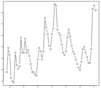
Figure2.2shows the average annual unemployment rates (given as a percentage of the civilian work force of age 16 years or over) in the U.S. in the years 1948-2011; the data are available from the U.S. Bureau of Labor Statistics. Assuming these data are a realization of a stationary process{Xt} (we provide some justification of this in what follows), we aim here to illustrate
interval estimates for the mean EXt=µannual unemployment rate as well as for the parameter θ = r(2)/r(1), where r(k) = Cov(X0, Xk), which we will show fits into the smooth model
framework described in Section2.2.2.2.
To obtain approximate 95% CIs for the mean parameter, we applied PBEL method as well as the BEL approach with OL or NOL blocks (denoted as BEL and NBEL, respectively) and the TBEL method. Intervals from BEL/NBEL/TBEL methods were computed over block sizes
b = 2,4,8, corresponding here to Cn1/3 with C = 0.5,1,2. Table 2.4 displays the resulting intervals. The PBEL interval emerges as a type of compromise between the CIs of other EL methods using block sizes b = 4 or 8. Figure 2.3 illustrates the shapes of the corresponding
case and that the BEL ratio has increasingly sharper tails for large block lengths. This visual illustration of the likelihood ratios is suggestive of how the BEL method can be sensitive to the block length choice.
The parameterθ=r(2)/r(1) fits into the smooth function model by definingYt= (P2i=0Xt+i/3,
P1
i=0Xt+iXt+1+i/2, XtXt+3), fort= 1, . . . ,62, and noting thatθ=H(E(Yt)) forH(x1, x2, x3) =
(x3−x21)/(x2−x21). Applying the EL methods to {Yt}, we obtained approximate 95% CIs for θ listed in Table2.5.
Regarding the unemployment rates in Figure2.2, model diagnostics indicate that an ARMA (1,1) model provides a reasonable fit for these data. Sample autocovariances are significantly zero and decay slowly at small lags, while the partial autocovariance is significantly non-zero at lag 1, suggesting a potential autoregressive component. Model selection criteria (e.g., AICC) support an ARMA(1,1) and residual diagnostics (e.g., sample autocovariances, Ljung-Box statistic) from the fitted model agree with white noise. Under an ARMA(1,1) model, the parameterθhere represents the corresponding AR model coefficient. Hence, for comparison to the EL intervals in Table2.5, we computed approximate 95% CIs forθbased on parametric fits in the ARMA(1,1) model by Hannan-Rissanen or (Gaussian) maximum likelihood estimation (cf. Brockwell and Davis, 2002), which were (0.367,0.827) and (0.434,0.898), respectively. The PBEL interval agrees with the parametric intervals, though with a slightly elongated lower endpoint. In this case, the PBEL interval appears again to be a blending of the other EL CIs and, as such, this interval turned out to be slightly more asymmetric than the other intervals, as seen in the likelihood plots of Figure 2.4.
2.4.2 Records of hemispheric temperatures
As mentioned at the end of Section2.2, the PBEL blocking scheme and likelihood formulation also applies to inference with general estimating functions (cf. Qin and Lawless, 1994; Kitamura, 1997) and stationary time series. In this section, we consider a small illustration of estimating functions in a regression setting.
details. The data, consisting of adjusted monthly temperature averages from 1850-2010, repre-sent a product of combining gridded surface air temperatures from global land station records, as well as marine data records, after correcting for non-climatic (e.g., instrumental) errors. For scientific reasons, the temperatures are then represented as anomalies (not actual tempera-tures), meaning that the data represent deviations from a mean temperature computed over a reference period (1961-1990) (cf. Brohan et. al.2006); in computing average monthly temper-atures, Jones et. al.1999 discuss how this adjustment reduces technical problems (e.g., due to differing station elevations or reporting discrepancies among countries). See Tingley (2011) for a statistical development in calculating climate anomalies.
Figure 2.5 shows annual average temperature anomalies for months December-January-February (DJF) and June-July-August (JJA) over the years 1850-2009. in both northern and southern hemispheres; DJF values are means of average temperature anomaly of December of the current year and January and February of the next year. To illustrate inference with general estimating functions, we consider fitting a simple linear modelYt=βXt+tfor predicting DJF
temperature anomalies{Yt}from JJA ones{Xt}(i.e., predicting winter/summer averages from
summer/winter averages, depending on the hemisphere). For this, we consider an estimating function g(Yt, Xt, β) = Xt(Yt −βXt), supposing E[g(Yt, Xt, β0)] = 0 at the true parameter
value. While the series in Figure 2.5 appear non-stationary, it is plausible that the series
Zt =g(Yt, Xt, β0) is stationary, as plots ofg(Yt, Xt,βˆ),t= 1850, . . . ,2009, using the ordinary
least squares (OLS) estimator ˆβ, suggest a stationary series with mean zero. From the overall variability explained in this OLS fit, JJA temperature anomalies appear to be better predictors of DJF anomalies in the southern hemisphere (with adjusted R-squared 0.930) than in the northern (with adjusted R-squared 0.623), which should then intuitively be reflected in the precision of interval estimates for β by hemisphere. We applied the PBEL method, using
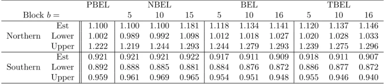
g(Yt, Xt, β) to replace Xt−µin EL function (2.3), and computed an approximate 90% CI for β, listed in Table 2.6. Table 2.6also includes CIs from other blockwise EL methods.
In this estimating function framework, the PBEL intervals also seem to be a mixture of CIs from other blockwise EL methods based on different block sizes, with shorter intervals for
bootstrap CIs for β are (1.017,1.262) in northern or (0.883,0.952) in southern hemispheres based resampling blocks from{(Yt, Xt)}of size 5 and computing bootstrap percentile intervals
forβ based on bootstrap OLS estimators ˆβ∗n. Among the EL intervals, the PBEL intervals tend to agree fairly well with the block bootstrap intervals, which are included here as a check because the block bootstrap is known to be valid for regression inference with potentially non-stationary data (cf. Fitzenberger, 1997) and uses/resamples data blocks which are fundamentally different than the data blocks used in the blockwise EL methods. That is, the latter use data blocks based on g(Yt, Xt, β) = Xt(Yt−βXt) to construct an EL function for inference about the
regressor slope β, while the block bootstrap reconstructs versions (Yt∗, Xt∗) of the original response/regressor series by resampling blocks of paired values (Yt, Xt) and then computing
subsequent bootstrap OLS estimators ˆβn∗ from the resampled data. The fact that the PBEL intervals are supported by a very form of block resampling provides some evidence that the method is valid and reasonable for these temperature anomaly data in the context of general estimation functions.
2.5 Conclusion remarks
We have introduced alternative version of blockwise empirical likelihood (BEL) that uses a non-standard blocking device, where data blocks do not have constant lengths for a given sample size, but rather increase in length through an arithmetic progression. Hence, no block selections are required and the blocks involved are implicity well-defined in this progressive block empirical likelihood (PBEL). Under conditions entailing weak dependence for stationary time series, the log-ratio statistic from the PBEL method has been shown to have a chi-square limit distribution, with some features resembling those found in EL with iid data (i.e., behavior of the log-ratio and Lagrange multiplier). While we have focused on inference on process means, or smooth functions of these, the blocking device presented here would remain valid for inference in other blockwise empirical likelihood scenarios involving estimating equations. Simulations have shown that the PBEL performs comparably to BEL when the later is based on a good block choice and often much better when an inadequate block selection is used. Because block
that the PBEL can have a practical advantage in being robust against against a choice of block size for capturing time dependence.
2.6 Proofs of main results
To establish Theorem1, we require some additional notation along with several initial, technical results stated in Lemma1below. Let E(Xt) =µ0 ∈Rdagain denote the true process mean and
recall Σ∞ ≡ P∞k=−∞r(k) is the sum of process autocovariances r(k) = Cov(X0, Xk), k ∈ Z,
where Zdenotes the set of integers. Recall nand N, respectively, denote the sample size and
the number of available progressive blocks, which satisfy√n/N →1 asn→ ∞by construction. For the progressive (centered) block sums Si,µ0 =
Pmin{i(i+1),n}
j=i(i−1)+1 (Xj−µ0),i= 1, . . . , N, define Zn ≡ max1≤i≤NkSi,µ0k as well as a block-based estimator ˆΣn ≡ n
−1PN
i=1Si,µ0S
T
i,µ0 of Σ∞. Let CH◦n denote the interior of the convex hull of points {Si,µ0}
N
i=1 ⊂ Rd and 0d denote the
zero vector inRd. In the following, unless indicated otherwise, limits→ denote convergence as
n→ ∞.
Lemma 1. Under the assumptions in Theorem 1, (a) n1/2( ¯Xn−µ0) d
→ Z ∼Normal(0,Σ∞);
(b) E(kSi,µ0k
4)≤Ci2, for a constantC >0 not depending onn or i= 1, . . . , N;
(c) Zn=oP(n1/2); (d)kΣˆn−Σ∞k=oP(1); and (e)P(0d∈CH◦n)→1.
Proof of Lemma 1. Part (a) follows from the central limit theorem for mixing processes
(cf. Ch. 16.3, Athreya and Lahiri, 2006), while part (b) is a moment bound on sums under Theorem 1 assumptions (cf. sec. 1.4.1, Doukhan, 1994). To show part (c), we use Jensen’s inequality and part (b) to bound
E(Zn)≤E N X i=1 kSi,µ0k 4 !1/4 ≤ " N X i=1 E(kSi,µ0k 4) #1/4 =O(N3/4) =o(n1/2),
using N/√n→1; part (c) then follows.
summa-a1≡ ∞ X k=1 kkr(k)k<∞, a2 ≡ X t1,t2,t3∈Z kcu(X0, Xt1, Xt2, Xt3)k<∞,
using Davydov’s inequality (cf. Doukhan, 1994, sec. 1.2.2; Athreya and Lahiri, 2006, Ch. 16.2). Then, for each blocki= 1, . . . , N−1, we can expand
1 2iE[Si,µ0S T i,µ0] = 2i X k=−2i 1−|k| 2i r(k) = Σ∞+Ri,
where the remainder satisfies kRik ≤ P|k|>2ikr(k)k + (2i)−1
P
k∈Z|k|kr(k)k ≤ i−1a1 and
E[SN,µ0S
T
N,µ0] = Σ∞+O(N) by Lemma1(b). From this, we may write
E[ ˆΣn] = 1 n N X i=1 2iE[Si,µ0S T i,µ0] 2i = Σ∞ N X i=1 2i n +O N n = Σ∞ (N + 1)N n +o(1)→Σ∞.
Also, for any fixed v∈Rd withkvk= 1,
Var(vTΣˆnv)≤ 1 n2 N X i=1 kSi,µ0k 4+ 2 n2 X 1≤i<j≤N |Cov[(vTSi,µ0) 2,(vTS j,µ0) 2]|=O(n−1/2),
which follows from bounding both sums above byO(N3/n2), using part (b) for the first sum and using that|Cov[(vTSi,µ0)
2,(vTS j,µ0) 2]|, 1≤i < j ≤N, is bounded by 2[Cov(vTSi,µ0, v TS j,µ0)] 2+|cu(vTS i,µ0, v TS i,µ0, v TS j,µ0, v TS j,µ0)| ≤2(a1) 2+ia 2
to handle the second sum. Hence, ˆΣn is MSE-consistent for Σ∞, proving part (d).
For part(e), fix v ∈ Sd = {x ∈
Rd : kxk = 1} in the unit sphere and define a type
of subsampling estimator ˆPn,v = N−1PNi=1I[(2i)−1/2vTSi,µ0 < 0] of the normal probability
P(vTZ <0), Z ∼N(0,Σ∞), where I[·] denotes the indicator function. By the distributional
convergence in part(a), we have
pi≡P((2i)−1/2vTSi,µ0 <0)→P(v
TZ <0)
as i → ∞. Hence, E[ ˆPn,v] = N1 PNi=1pi → P(vTZ < 0) as n → ∞ as a Cesaro mean.
Additionally, Davydov’s inequality with the mixing coefficient imply that Var[ ˆPn,v]≤N−1(1 +
4P∞
k=1α(k)δ/(δ+6)) =o(1), so that ˆPn,v p
open balls of radius 1/m around v ∈ Cm cover Sd, and one may choose C m ⊂ Cm+1. Since ˆ Pn,v p → P(vTZ < 0) forv ∈ S
m=1Cm, the latter being a countable set, for any subsequence
{nj}of{n}, there exists a further subsequence{nk} ⊂ {nj}where, ˆPnk,v→P(v
TZ <0) holds
for allv∈S
m=1Cm, almost surely (a.s.). This in turn implies supv∈Sd|Pˆnk,v−P(vTZ <0)| →0 a.s., which is equivalent to supv∈Sd|Pˆn,v−P(vTZ <0)|=oP(1). The positivity of Σ∞ implies
that, for some C > 0, infv∈SdP(vTZ < 0) > C holds (cf. Lemma 2, Owen, 1990), so that
P(infv∈SdPˆn,v > C/2)→1.
Finally, if 0d 6∈ CH◦n, then ˜vTSi,µ0 ≥ 0 holds for some kv˜k = 1∈ R
d and all i = 1, . . . , N
by the supporting/separating hyperplane theorem, which implies that ˆPn,˜v = 0. Hence, P(0d6∈CH◦n)≤P(infv∈SdPˆn,v ≤C/2)→0, proving part (e).
2.6.1 Proof of Theorem 1
Assuming 0d∈CH◦n(which happens with arbitrarily large probability asn→ ∞by Lemma1(e)), Rn(µ0) is finitely positive and equals Rn(µ0) = QNi=1(1 +γi)−1 (Owen, 1990, p. 100), where γi =Si,µT 0λn and λn∈R d satisfies 0d= 1 n N X i=1 Si,µ0 1 +γi = ( ¯Xn−µ0)− 1 n N X i=1 Si,µ0S T i,µ0λn 1 +γi . (2.5)
Writing λn = kλnkvn for some vn ∈ Rd, kvnk = 1 and then multiplying (2.5) by −vn, we
may obtain kX¯n − µ0k ≥ (1 + kλnkZn)−1kλnkvTΣˆnv. Applying Lemma 1(a),(c),(d) and
letting kΣ∞k2 > 0 denote the spectral norm of Σ∞, this implies that n1/2kX¯n −µ0k ≤ n1/2kλnk[kΣ∞k2 +oP(1)] holds with arbitrarily large probability as n → ∞, or that λn = OP(n−1/2). By Lemma 1(c), we also then have that max1≤i≤N|γi| ≤Znkλnk =oP(1). With
probability approaching 1 as n→ ∞, we may expand (2.5) to produce
λn= ˆΣ−n1( ¯Xn−µ0+βn), βn≡n−1 N
X
i=1
γi2Si,µ0/(1 +γi), (2.6)
(using Lemma 1(d) above) and bound
by Holder’s inequality and Lemma1(b).
When max1≤i≤N|γi| ≤ Znkλnk <1, Taylor’s expansion gives log(1 +γi) =γi−γ2i/2 +ηi
with |ηi| ≤ kλnk3kSi,µ0k
3/(1− kλkZ
n)3, i= 1, . . . , N. Note that PNi=1|ηi| ≤ kλnk3nBn/(1−
kλnkZn)3 =OP(n−3/2)OP(n5/4)OP(1) =OP(n−1/4). Using this with (2.6),kβnk=OP(n−3/4),
PN
i=1Si,µ0 =n( ¯Xn−µ0) and −2 logRn(µ0) = 2
Pn
i=1log(1 +γi) =
PN
i=1(2γi−γi2 + 2ηi) for γi = Si,µT 0λn, we have the following expansion (holding with arbitrarily high probability for largen) −2 logRn(µ0) = n( ¯Xn−µ0)TΣˆ−n1( ¯Xn−µ0)−nβnTΣˆ −1 n βn+ 2 N X i=1 ηi = n( ¯Xn−µ0) ˆΣ−n1( ¯Xn−µ0) +OP(n−1/4).
Lemma1(a) and (d) with Slutsky’s theorem complete the proof.
2.6.2 Proof of Theorem 2
We sketch the proof, modifying arguments given in Hall and La Scala (1990, Theorem 1). If we define a set Mn ≡ {µ ∈ Rd : Rn(µ) ≥ Rn(µ0)} of mean values with an PBEL ratio at
least as great as the true meanµ0, then it can be shown that supµ∈Mnkµ−µ0k=Op(n
−1/2)
(following from the arguments below, i.e., forµ=µ0+n−1/2Σ∞1/2w withw∈Rd,−2 logRn(µ)
has a non-central chi-square limit with non-centrality parameter kwk). Hence, it suffices to establish a limit distribution based onRn,C(θ0) = sup{Rn(µ) :H(µ) =θ0,kµ−µ0k ≤Cn−1/2}
for a fixed constant C >0, asRn,C(θ0) andRn(θ0) will asymptotically match with arbitrarily
high probability for largeC.
Defining a subsampling-type estimator ˆPµ,n,v =N−1
PN
i=1I[(2i)
−1/2vTS
i,µ0 <0] forv∈ S
d
as in the proof of Lemma1(e), it can be shown that supv∈Sd,kµ−µ
0k≤Cn−1/2|Pˆµ,n,v−P(v 0Z <0)| is bounded by sup v∈Sd 1 N N X i=1
I[−C(2i/n)1/2≤(2i)−1/2vTSi,µ0 <0] + sup
v∈Sd
|Pˆµ0,n,v−P(v
0Z <0)|=o
n → ∞. With arbitrarily high probability for large n, we may then assume an expansion logRn(µ) = −
Pn
i=1log(1 +γi,µ) holds for each µ ∈ Rd, kµ−µ0k ≤ Cn−1/2, where γi,µ = λTn,µSi,µ ∈(−1,1) and λn,µ ∈Rd satisfy
0d= ( ¯Xn−µ)− 1 n N X i=1 Si,µSi,µT λn,µ 1 +γi,µ ,
analogously to (2.5). Defining ¯Zn = supkµ−µ0k≤Cn−1/2max1≤i≤nkSi,µk, it follows that ¯Zn =
op(n1/2) by Lemma1(c) and, defining ˆΣn,µ=n−1Pni=1Si,µSi,µT , Lemma 1(d) then establishes
sup
kµ−µ0k≤Cn−1/2
kΣˆn,µ−Σ∞k=op(1) +Op(n−3/2Z¯nN2) =op(1).
As in the proof of Theorem 1, one may then determine supkµ−µ
0k≤Cn−1/2kλn,µk =Op(n
−1/2)
and λn,µ= ˆΣ−n,µ1( ¯Xn−µ+βn,µ), where supkµ−µ0k≤Cn−1/2kβn,µk=Op(n
−3/4). It also similarly
follows that−2 logRn(µ) =n( ¯X−µ)TΣ−∞1( ¯X−µ)+En,µwhere supkµ−µ0k≤Cn−1/2|En,µ|=op(1). Letting ∇µ ≡[∂Hi(µ)/∂µj]i=1,...,p;j=1,...,d and noting a Taylor expansion in a neighborhood of µ0givesH(µ0+ν)−θ0 =Dν forDν ≡
R1
0 ∇µ0+tνdt→ ∇µ0 askνk →0, we may use Lemma1(a) to write −2 logRn,C(θ0) = inf{−2 logRn(µ) :H(µ) =θ0,kµ−µ0k ≤Cn−1/2} = inf{n( ¯X−µ0+ν)TΣ−∞1( ¯X−µ0+ν) :Dνν = 0p,kνk ≤Cn−1/2}+op(1) d → inf{(Σ−∞1/2Z+ν)T(Σ∞−1/2Z+ν) :ν ∈Rd,∇µ0Σ 1/2 ∞ ν= 0p} = (Σ−∞1/2Z)TPΣ1/2 ∞ ∇Tµ0 (Σ−∞1/2Z) d = χ2p, whereP Σ1/2∞ ∇Tµ0
denotes the projection matrix for the column space inRdspanned by Σ1∞/2∇Tµ0. Since Σ−∞1/2Z is distributed as a vector of d independent standard normals and PΣ1/2
∞ ∇Tµ0 is idempotent with rankp, the chi-square distributional limit follows.
Athreya, K.B. and Lahiri, S.N. (2006). Measure theory and probability theory. Springer, New York.
Bravo, F. (2005). Blockwise empirical entropy tests for time series regressions. J. Time Series Anal.,26, 185-210.
Bravo, F. (2009). Blockwise generalized empirical likelihood inference for non-linear dynamic moment conditions models.Econometrics Journal,12, 208-231.
Brohan, P., Kennedy, J.J., Harris, I., Tett, S.F.B. and Jones, P.D. (2006). Uncertainty estimates in regional and global observed temperature changes: a new dataset from 1850. J. Geophysical Research,111, D12106,
Brockwell, P. J. and Davis, R. A. (2002). Introduction to time series and forecasting. Second Edition, Springer, New York.
Carlstein, E. (1986). The use of subseries methods for estimating the variance of a general statistic from a stationary time series. Ann. Statist.,14, 1171-1179.
Chen S. X. and Wong C. M. (2009). Smoothed block empirical likelihood for quantiles of weakly dependent processes.Statistic Sinica,19, 71-81.
Doukhan, P. (1994). Mixing: Properties and Examples. Lecture Notes in Statistics, 85. New York: Springer-Verlag.
Fitzenberger, B. (1997). The moving blocks bootstrap and robust inference for linear least squares and quantile regressions.J. Econometrics,82, 235-287.
Hall, P. (1985). Resampling a coverage pattern. Stochastic Process. Appl.,20, 231-246. Hall, P. and La Scala, B. (1990). Methodology and algorithms of empirical likelihood.Internat.
Statist. Rev.58, 109-127.
Hall, P., Horowitz, J. and Jing, B. (1992). On blocking rules for the bootstrap with dependent data. Biometriak 82, 561-574.
Jones, P.D., New, M., Parker, D.E., Martin, S. and Rigor, I.G. (1999). Surface air temperature and its variations over the last 150 years.Reviews of Geophysics,37, 173-199.
pendium of Data on Global Change. Carbon Dioxide Information Analysis Center, Oak Ridge National Laboratory, U.S. Department of Energy, Oak Ridge, Tenn., U.S.A. doi: 10.3334/CDIAC/cli.002
Kitamura, Y. (1997). Empirical likelihood methods with weakly dependent processes. Ann. Statist.,25, 2084-2102.
K¨unsch, H. R. (1989). The jackknife and bootstrap for general stationary observations.Ann. Statist.,17, 1217-1261.
Lahiri, S. N. (2003). Resampling methods for dependent data.Springer, New York.
Lei, Q. and Qin, Y. (2011). Empirical likelihood for quantiles under negatively associated samples.J. Statist. Plann. Inference,141, 1325-1332.
Lin, L. and Zhang, R. (2001). Blockwise empirical Euclidean likelihood for weakly dependent processes.Statist. Prob. Lett,53, 143-152.
Liu, R. Y. and Singh, K. (1992). Moving blocks jackknife and bootstrap capture weak de-pendence. In Exploring the Limits of Bootstrap, 225-248, R. LePage and L. Billard (editors). John Wiley & Sons, New York.
Nordman, D. J., Sibbertsen, P. and Lahiri, S. N. (2007). Empirical likelihood for the mean under long-range dependence. J. Time Series Anal.,28, 576-599.
Nordman, D. J. (2009). Tapered empirical likelihood for time series data in time- and frequency-domains.Biometrika,96, 119–132.
Owen, A. B. (1988). Empirical likelihood ratio confidence intervals for a single functional.
Biometrika,75, 237-249.
Owen, A. B. (1990). Empirical likelihood confidence regions.Ann. Statist.,18, 90-120. Owen, A. B. (2001). Empirical likelihood.Chapman & Hall, London.
Politis, D. N. and Romano, J. P. (1993). On the sample variance of linear statistics derived from mixing sequences.Stochastic Processes Appl.,45, 155-167.
Politis, D. N., Romano, J. P., and Wolf, M. (1999).Subsampling. Springer-Verlag, New York. Qin, J. and Lawless, J. (1994) Empirical likelihood and general estimating equations. Ann.
applications to the instrumental temperature record.Journal of Climate(in press). Wilks, S. S. (1938). The large-sample distribution of the likelihood ratio for testing composite
hypotheses. Ann. Math. Statist.,9, 60-62.
Wu, R. and Cao, J. (2011). Blockwise empirical likelihood for time series of counts. J. Multi-variate Anal. 102, 661-673.
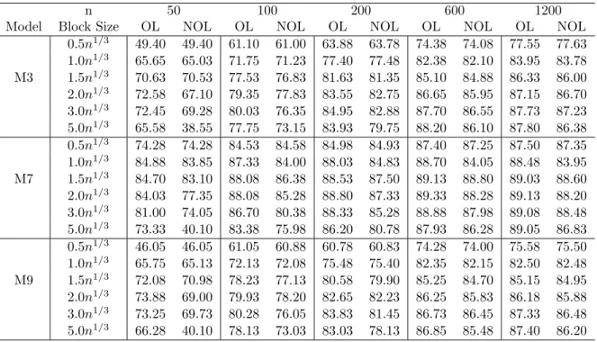
Table 2.2 Empirical coverage probabilities for 90% confidence intervals for the process mean based on BEL, with either overlapping (OL) or non-overlapping (NOL) blocks. Results are presented over three data-generating models, and various block sizesb, and sample sizes n.
n 50 100 200 600 1200
Model Block Size OL NOL OL NOL OL NOL OL NOL OL NOL
0.5n1/3 49.40 49.40 61.10 61.00 63.88 63.78 74.38 74.08 77.55 77.63 1.0n1/3 65.65 65.03 71.75 71.23 77.40 77.48 82.38 82.10 83.95 83.78 M3 1.5n1/3 70.63 70.53 77.53 76.83 81.63 81.35 85.10 84.88 86.33 86.00 2.0n1/3 72.58 67.10 79.35 77.83 83.55 82.75 86.65 85.95 87.15 86.70 3.0n1/3 72.45 69.28 80.03 76.35 84.95 82.88 87.70 86.55 87.73 87.23 5.0n1/3 65.58 38.55 77.75 73.15 83.93 79.75 88.20 86.10 87.80 86.38 0.5n1/3 74.28 74.28 84.53 84.58 84.98 84.93 87.40 87.25 87.50 87.35 1.0n1/3 84.88 83.85 87.33 84.00 88.03 84.83 88.70 84.05 88.48 83.95 M7 1.5n1/3 84.70 83.10 88.08 86.38 88.53 87.50 89.13 88.80 89.03 88.60 2.0n1/3 84.03 77.35 88.08 85.28 88.80 87.33 89.33 88.28 89.13 88.20 3.0n1/3 81.00 74.05 86.70 80.38 88.33 85.28 88.88 87.98 89.08 88.48 5.0n1/3 73.33 40.10 83.38 75.98 86.20 80.78 87.93 86.28 89.05 86.83 0.5n1/3 46.05 46.05 61.05 60.88 60.78 60.83 74.28 74.00 75.58 75.50 1.0n1/3 65.75 65.13 72.13 72.08 75.48 75.40 82.35 82.15 82.50 82.48 M9 1.5n1/3 72.08 70.98 78.23 77.13 80.58 79.90 85.25 84.70 85.15 84.95 2.0n1/3 73.88 69.00 79.93 78.20 82.65 82.23 86.25 85.83 86.18 85.88 3.0n1/3 73.25 69.73 80.28 76.05 83.83 81.45 86.73 86.45 87.33 86.48 5.0n1/3 66.28 40.10 78.13 73.03 83.03 78.13 86.85 85.48 87.40 86.20
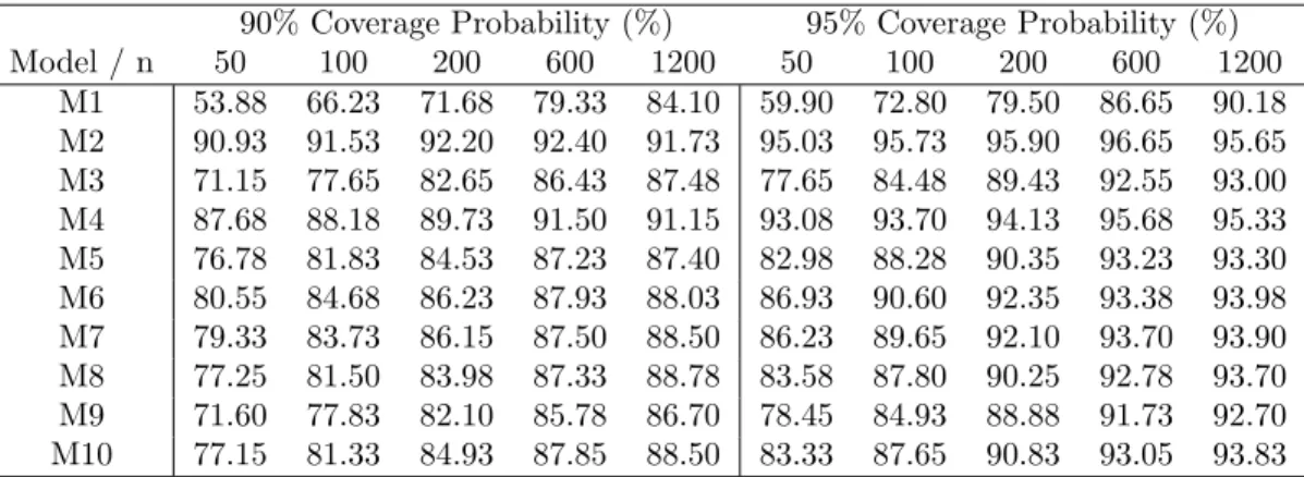
Table 2.3 Coverage probabilities for nominal 90% and 95% progressive block empirical likeli-hood (PBEL) confidence intervals for the process mean of ten time series processes over variance sample sizes n(based on 4000 simulations).
90% Coverage Probability (%) 95% Coverage Probability (%)
Model/n 50 100 200 600 1200 50 100 200 600 1200 M1 53.88 66.23 71.68 79.33 84.10 59.90 72.80 79.50 86.65 90.18 M2 90.93 91.53 92.20 92.40 91.73 95.03 95.73 95.90 96.65 95.65 M3 71.15 77.65 82.65 86.43 87.48 77.65 84.48 89.43 92.55 93.00 M4 87.68 88.18 89.73 91.50 91.15 93.08 93.70 94.13 95.68 95.33 M5 76.78 81.83 84.53 87.23 87.40 82.98 88.28 90.35 93.23 93.30 M6 80.55 84.68 86.23 87.93 88.03 86.93 90.60 92.35 93.38 93.98 M7 79.33 83.73 86.15 87.50 88.50 86.23 89.65 92.10 93.70 93.90 M8 77.25 81.50 83.98 87.33 88.78 83.58 87.80 90.25 92.78 93.70 M9 71.60 77.83 82.10 85.78 86.70 78.45 84.93 88.88 91.73 92.70 M10 77.15 81.33 84.93 87.85 88.50 83.33 87.65 90.83 93.05 93.83
Table 2.4 Approximate 95% CIs (Lower,Upper) for the mean annual unemployment rate along with point estimates (Est) as maximizers of respective EL functions.
PBEL NBEL BEL TBEL
Blockb= 2 4 8 2 4 8 2 4 8
Est 5.767 5.767 5.767 5.767 5.756 5.704 5.726 5.756 5.707 5.693
Lower 5.078 5.265 5.182 5.042 5.259 5.102 5.034 5.259 5.135 5.015
Upper 6.465 6.347 6.499 6.576 6.331 6.408 6.538 6.331 6.379 6.501
Table 2.5 Approximate 95% intervals (Lower,Upper) for the parameter θ=r(2)/r(1) (corre-sponding to the AR coefficient in an ARMA(1,1) model) along with point estimates (Est) as maximizers of respective EL functions.
PBEL NBEL BEL TBEL
Blockb= 2 4 8 2 4 8 2 4 8
Est 0.571 0.571 0.661 0.606 0.584 0.658 0.652 0.584 0.669 0.677
Lower 0.159 0.179 0.331 0.332 0.157 0.301 0.291 0.157 0.285 0.362
Table 2.6 Estimated regression coefficient and approximate 90% CIs forβ(in linear prediction of DJF temperature anomalies from JJA records over 1850-2009) with different EL methods and block sizes b= 5,10,15 (corresponding toCn1/3 forC= 1,2,3).
PBEL NBEL BEL TBEL
Blockb= 5 10 15 5 10 16 5 10 16 Est 1.100 1.100 1.100 1.181 1.118 1.134 1.141 1.120 1.137 1.146 Northern Lower 1.002 0.989 0.992 1.098 1.012 1.018 1.027 1.020 1.028 1.033 Upper 1.222 1.219 1.244 1.293 1.244 1.279 1.293 1.239 1.275 1.296 Est 0.921 0.921 0.921 0.922 0.917 0.911 0.909 0.918 0.911 0.907 Southern Lower 0.892 0.888 0.885 0.881 0.884 0.876 0.872 0.886 0.877 0.872 Upper 0.959 0.961 0.969 0.965 0.954 0.951 0.948 0.955 0.946 0.940
Figure 2.1 Plot of differences between the nominal level and actual coverage rates for 90% CIs for the process mean; positive differences indicate undercoverage. Results are presented for three sample sizes n and ten data-generating models (denoted M1-M10). Coverage differences for the PBEL method are indicated by ◦; cov-erage differences for BEL and TBEL methods based on block sizes b = Cn1/3
(C = 0.5,1.0,1.5,2.0,3.0,5.0) are indicated by “EL1-EL6” and “TEL1-TEL6.”
n= 50 0.0 0.2 0.4 0.6 EL1 EL1 EL1 EL1 EL1 EL1 EL1 EL1 EL1 EL1 TEL1 TEL1 TEL1 TEL1 TEL1 TEL1 TEL1 TEL1 TEL1 TEL1 EL2 EL2 EL2 EL2 EL2 EL2 EL2 EL2 EL2 EL2 TEL2 TEL2 TEL2 TEL2 TEL2 TEL2 TEL2 TEL2 TEL2 TEL2 EL3 EL3 EL3 EL3 EL3 EL3 EL3 EL3 EL3 EL3 TEL3 TEL3 TEL3 TEL3 TEL3 TEL3 TEL3 TEL3 TEL3 TEL3 EL4 EL4 EL4 EL4 EL4 EL4 EL4 EL4 EL4 EL4 TEL4 TEL4 TEL4 TEL4 TEL4 TEL4 TEL4 TEL4 TEL4 TEL4 EL5 EL5 EL5 EL5 EL5 EL5 EL5 EL5 EL5 EL5 TEL5 TEL5 TEL5 TEL5 TEL5
TEL5 TEL5 TEL5
TEL5 TEL5 EL6 EL6 EL6 EL6 EL6 EL6 EL6 EL6 EL6 EL6 TEL6 TEL6 TEL6 TEL6 TEL6
TEL6 TEL6 TEL6
TEL6 TEL6 ● ● ● ● ● ● ● ● ● ● M1 M2 M3 M4 M5 M6 M7 M8 M9 M10 n= 200 −0.1 0.0 0.1 0.2 0.3 0.4 0.5 EL1 EL1 EL1 EL1 EL1 EL1 EL1 EL1 EL1 EL1 TEL1 TEL1 TEL1 TEL1 TEL1 TEL1 TEL1 TEL1 TEL1 TEL1 EL2 EL2 EL2 EL2 EL2 EL2 EL2 EL2 EL2 EL2 TEL2 TEL2 TEL2 TEL2 TEL2 TEL2 TEL2 TEL2 TEL2 TEL2 EL3 EL3 EL3 EL3 EL3 EL3 EL3 EL3 EL3 EL3 TEL3 TEL3 TEL3 TEL3 TEL3 TEL3 TEL3 TEL3 TEL3 TEL3 EL4 EL4 EL4 EL4 EL4 EL4 EL4 EL4 EL4 EL4 TEL4 TEL4 TEL4 TEL4 TEL4 TEL4 TEL4 TEL4 TEL4 TEL4 EL5 EL5 EL5 EL5 EL5 EL5 EL5
EL5 EL5 EL5 TEL5
TEL5
TEL5
TEL5 TEL5 TEL5 TEL5 TEL5
TEL5 TEL5 EL6 EL6 EL6 EL6 EL6
EL6 EL6 EL6
EL6 EL6 TEL6
TEL6 TEL6
TEL6 TEL6 TEL6 TEL6 TEL6 TEL6 TEL6 ● ● ● ● ● ● ● ● ● ● M1 M2 M3 M4 M5 M6 M7 M8 M9 M10 n= 1200 −0.1 0.0 0.1 0.2 0.3 0.4 EL1 EL1 EL1 EL1 EL1 EL1 EL1 EL1 EL1 EL1 TEL1 TEL1 TEL1 TEL1 TEL1 TEL1 TEL1 TEL1 TEL1 TEL1 EL2 EL2 EL2 EL2 EL2
EL2 EL2 EL2
EL2 EL2 TEL2 TEL2 TEL2 TEL2 TEL2
TEL2 TEL2 TEL2
TEL2 TEL2 EL3 EL3 EL3 EL3 EL3 EL3 EL3 EL3 EL3 EL3 TEL3 TEL3 TEL3 TEL3
TEL3 TEL3 TEL3 TEL3
TEL3 TEL3 EL4 EL4 EL4 EL4 EL4 EL4 EL4 EL4 EL4 EL4 TEL4 TEL4 TEL4 TEL4
TEL4 TEL4 TEL4 TEL4
TEL4
TEL4 EL5
EL5 EL5
EL5
EL5 EL5 EL5 EL5 EL5
EL5 TEL5
TEL5 TEL5
TEL5
TEL5 TEL5 TEL5 TEL5 TEL5 TEL5 EL6
EL6
EL6
EL6
EL6 EL6 EL6 EL6 EL6
EL6 TEL6
TEL6 TEL6
TEL6 TEL6 TEL6 TEL6 TEL6 TEL6 TEL6 ● ● ● ● ● ● ● ● ● ● M1 M2 M3 M4 M5 M6 M7 M8 M9 M10
Figure 2.2 Plot of U.S. annual average unemployment rates from 1948-2011. ● ● ● ● ●● ● ● ● ● ● ●● ● ● ● ● ● ●● ●● ● ● ● ● ● ● ● ● ● ● ● ● ● ● ● ● ● ● ● ● ● ● ● ● ● ● ● ● ● ● ● ● ● ● ● ● ●● ● ● ● ● 1950 1960 1970 1980 1990 2000 2010 3 4 5 6 7 8 9 Year U.S. Unemplo yment Rate (%)
Figure 2.3 Plots of EL ratios for the mean µ annual unemployment rate. Solid horizontal lines in each plot indicate the calibration cut-off for defining 95% CIs.
PBEL BEL,b= 2 5.0 5.5 6.0 6.5 0.0 0.2 0.4 0.6 0.8 1.0 mu EL function f or theta 5.0 5.5 6.0 6.5 0.0 0.2 0.4 0.6 0.8 1.0 mu EL function f or theta BEL,b= 4 BEL,b= 8 5.0 5.5 6.0 6.5 0.0 0.2 0.4 0.6 0.8 1.0 mu EL function f or theta 5.0 5.5 6.0 6.5 0.0 0.2 0.4 0.6 0.8 1.0 mu EL function f or theta
Figure 2.4 Plots of EL ratios for θ = r(2)/r(1) from unemployment data. Solid horizontal lines in each plot indicate the calibration cut-off for defining 95% CIs.
PBEL BEL,b= 2 0.0 0.2 0.4 0.6 0.8 1.0 1.2 0.0 0.2 0.4 0.6 0.8 1.0 theta EL function f or theta 0.0 0.2 0.4 0.6 0.8 1.0 1.2 0.0 0.2 0.4 0.6 0.8 1.0 theta EL function f or theta BEL,b= 4 BEL,b= 8 0.0 0.2 0.4 0.6 0.8 1.0 1.2 0.0 0.2 0.4 0.6 0.8 1.0 theta EL function f or theta 0.0 0.2 0.4 0.6 0.8 1.0 1.2 0.0 0.2 0.4 0.6 0.8 1.0 theta EL function f or theta
Figure 2.5 Plots of average annual seasonal temperature anomalies for northern and southern hemispheres over the years 1850-2009, for seasons/months DJF (−) and JJA (· · ·).
Northern Hemisphere Southern Hemisphere
1850 1900 1950 2000 −1.0 −0.5 0.0 0.5 year A v er age ann ual temper atre anomalies 1850 1900 1950 2000 −0.6 −0.4 −0.2 0.0 0.2 0.4 year A v er age ann ual temper atre anomalies
CHAPTER 3. PROPERTIES OF A BLOCK BOOTSTRAP UNDER LONG-RANGE DEPENDENCE
A paper to be published to Sankhya in November, 2011
Young Min Kim and Daniel J. Nordman
Abstract
The block bootstrap has been largely developed for weakly dependent time processes and, in this context, much research has focused on the large-sample properties of block bootstrap inference about sample means. This work validates the block bootstrap for distribution estimation with stationary, linear processes exhibiting strong dependence. For estimating the sample mean’s variance under long-memory, explicit expressions are also provided for the bias and variance of moving and non-overlapping block bootstrap estimators. These differ critically from the weak dependence setting and optimal blocks decrease in size as the strong dependence increases. The findings in distribution and variance estimation are then illustrated using simulation.
Key Words: Block size; Confidence interval; Sample average; Variance estimation
3.1 Introduction
Block bootstrap methods for time series involve resampling data blocks to capture time de-pendence, which provided a breakthrough in bootstrap formulation following Singh’s (1981)
under dependence. While other time series bootstraps have become available, such as the sieve bootstrap (B¨uhlmann, 1997) and frequency-domain bootstrap (Kreiss and Paparoditis, 2003), the appeal of the block bootstrap has been its general validity over a wide range of time pro-cesses. Additionally, the type of block resampling flexibly allows for different block bootstraps, such as the moving block bootstrap (MBB) of K¨unsch (1989) and Liu and Singh (1992) and the non-overlapping block bootstrap (NBB) of Carlstein (1986) among several others. How-ever, most developments for the block bootstrap have treated only weakly dependent data. One exception is due to Lahiri (1993) who showed that the MBB could fail in approximating sample means for a category of strongly or long-range dependent (LRD) processes generated by transformations of Gaussian series. This finding appears to have largely deflated confidence in the block bootstrap for long-range dependence (LRD).
Our goal here is to establish block bootstrap inference about the sample mean for a differ-ent, but practically broad, class of stationary linear processes exhibiting LRD which includes popular models for LRD such as fractional Gaussian processes (Mandelbrot and Van Ness, 1968) and fractional autoregressive integrated moving averages (Adenstedt, 1974; Granger and Joyeux, 1980; and Hosking, 1981). For these processes, we show MBB and NBB methods to be consistent for distribution estimation under mild and flexible conditions entailing LRD. In particular, these conditions permit general filter coefficients for defining the linear process and also allow for weak dependence, establishing the block bootstrap without the more usual mixing assumptions in this case. The former implies that the block bootstrap may be more widely valid under LRD than the sieve bootstrap, which has recently been justified for causal linear LRD series (Kapetanios and Psaradakis, 2006; Poskitt, 2007).
We also develop the large sample properties of block bootstrap variance estimators for the sample mean under LRD. While a great deal of research has focused on this problem in the weak dependence case (K¨unsch, 1989; Hall, Horowitz and Jing, 1995; Lahiri, 1999; Politis and White, 2004), little has been known about block bootstrap performance under strong dependence. We provide detailed expressions for the bias and variance of MBB and NBB estimators under LRD, and these findings are somewhat surprising. It turns out that, in contrast to weak dependence