Spatial Dynamics in Fisheries Stock Assessment

The University of Maine

DigitalCommons@UMaine

University of Maine Office of Research and

Sponsored Programs: Grant Reports

Special Collections

8-25-2014

Spatial Dynamics in Fisheries Stock Assessment

Yong Chen

Principal Investigator; University of Maine, Orono

, [email protected]

Follow this and additional works at:

https://digitalcommons.library.umaine.edu/orsp_reports

Part of the

Agricultural and Resource Economics Commons, and the

Aquaculture and Fisheries

Commons

This Open-Access Report is brought to you for free and open access by DigitalCommons@UMaine. It has been accepted for inclusion in University of

Recommended Citation

Chen, Yong, "Spatial Dynamics in Fisheries Stock Assessment" (2014).University of Maine Office of Research and Sponsored Programs: Grant Reports. 6.

A Final R e p o rt*

for

N M F S -S e a Grant Graduate Fellowship in Population Dynamics

NA10OAR4170237

Sp atial D ynam ics in F ish e rie s Sto ck A sse ssm e n t

(For the time period June 1, 2010 to May 31, 2014)

Fellow: Samuel Truesdell, Ph.D student in Fisheries Population Dynamics,

225 Libby Hall, School of Marine Sciences, University of Maine, Orono, ME 04469

Tel: (207) 581-4405, e-mail: [email protected]

Faculty Advisor: Dr. Yong Chen, Professor for Fisheries Population Dynamics, 218 Libby Hall,

School of Marine Sciences, University of Maine, Orono, ME 04469

Tel: (207) 581-4303, Fax: (207) 581-4990, e-mail: [email protected]

NMFS Mentor: Dr. Dvora Hart, Population Dynamics Branch, Northeast Fisheries Science

Center, 166 Water Street, Woods Hole, MA 02543,

e-mail: [email protected], Tel: 508-495-2369, Fax: 508-495-2393

*This report is derived from the fellow's PhD dissertation submitted to the University of Maine to meet the partial requirement of the fellow's PhD program.

Table o f Contents

Selected relevant activities during the fellowship p erio d :... iii

1 Background and objectives... 1

1.1 Introduction...1

1.2 Spatial distribution of fishing fle e ts...1

1.3 Objective...2

2 Spatial heterogeneity in a Y/R co n te xt... 3

2.1 Introduction...3

2.2 Methods...4

2.3 Results...7

2.4 Discussion...9

3 Extending effort heterogeneity to more complex m odels... 12

3.1 Introduction... 12

3.2 Methods... 13

3.3 Results... 26

Selected re le va n t a ctiv itie s during th e fe llo w sh ip period:

• Completed PhD requirements at University of Maine

• Traveled to NEFSC multiple times per year to meet with NMFS mentor • 32 days at sea on NMFS scallop surveys 2011-2013

• Lead scientist on Maine state scallop surveys 2011-2013

• Lead scientist on Maine DMR/University of Maine joint survey of the Northern Gulf of Maine scallop management area (2012)

• Worked on the University of Maine's sentinel longline/jigging groundfish survey

• Assisted in the design and implementation of a scallop dredge efficiency study for the state of Maine (2012)

• Supervised an University of Maine undergraduate in organizing the Maine DMR's scallop archives into a database

• Presented research at annual fellows meeting (2011-2013), annual University of Maine School of Marine Sciences Symposium (2011-2013), at the Canadian Conference for Fisheries Research (2011), invited presentations at Shanghai Ocean University and Ocean University of China (2011), and at the International Pectinid Workshop (2011)

• Supervised four University of Maine undergraduate students collecting data on scallop growth increments

• Lectured in SMS 562 Fisheries Population Dynamics (2010-2013), SMS 321 Introduction to Fisheries Science (2011), and SMS 402 Oceans and Climate Change (2011)

• Submitted papers on the Northern Gulf of Maine scallop survey and on the effects of heterogeneity in growth and fishing effort on Yield per Recruit models

• Published papers on the impacts of stock mixing on the assessment of Atlantic cod in the Gulf of Maine and on the effects of fish aggregation devices on tuna behavior in the western Pacific Ocean.

• Designed and conducted the survey of scallop resources in the northern Gulf of Maine federal waters and undertook the data analysis for developing catch quota for the scallop in the northern Gulf of Maine federal waters.

• Completed analysis for the New England Fishery Management Council that used statistical models to describe the distribution of juvenile cod and yellowtail flounder (2013)

1 Background and objectives

1.1 Introduction

Most fisheries stock assessments assume that the spatial distribution of fish and/or fishing effort is random (Hilborn and Walters 1992), even though this is rarely the case (Paloheimo and Dickie 1964, Caddy 1975, Hilborn and Walters 1992, Tilzey 1994, Hutchings 1996, Chen et al. 1998, Hart 2001). The target stock is often aggregated and the distribution of fishing effort reflects this spatial pattern, along with other factors such as management restrictions, distance to port, vessel size, and the experience and habits of individual fishers. This often results in high spatial variation in fishing effort and mortality.

Ignoring this spatial variation can lead to serious biases in estimates of fishing mortality and yield (Hart 2001). Additionally, the non-random spatial distribution of fish and fishing effort makes the interpretation of commercial catch rate (i.e, catch-per-unit-effort or CPUE) difficult (Paloheimo and Dickie 1964, Cooke and Beddington, 1984, NRC 1999). These indices are often used as an abundance index in stock assessment and used as an index in monitoring fish stocks. The targeted deployment of fishing effort often makes the observed CPUE unchanged and even increasing even if the stock size decreases until a point when the stock is at very low level (Hilborn and Walters 1992, Rose and Kulka 1999). Misinterpretation of CPUE indices has been a factor in the collapse of a number of fish stocks, most prominently northern cod (Hilborn and Walters 1992, Hutchings 1996, W alters and Maguire 1996, Rose and Kulka 1999). For these reasons, understanding spatial dynamics of a fishery is an important issue in fisheries management; management that does not consider the spatial dynamics of a fishery may be less successful in optimizing harvest and building an understanding of the interactions between the fishery and other environmental variables (Caddy 1975, Walters and Maguire 1996, Atkinson et al. 1997, NRC 1999, Hart 2001).

Most stock assessments lack a spatial component due, in part, to limited spatially-explicit information regarding the distribution of fishing effort. However, vessel monitoring systems (VMS) that give detailed and accurate information about the positions of fishing vessels are increasingly being used as a fishery enforcement tool. These same data can be employed by stock assessment scientists to characterize the spatial structure of a fishery. Such information can be used as a basis for spatially- explicit models for stock assessment and management.

1.2 Spatial distribution of fishing fleets

Heterogeneity in fishery systems is a mixture of natural and human factors. The natural component is the environmentally or stochastically determined distribution of individuals and their attributes in space. Densities and characteristics of the target animal are influenced by their local conditions that are reflective of the quality of their environment (MacCall, 1989). Heterogeneity in fishing activity (the human component) is a result of harvesters' attempts to maximize their utility, typically by optimizing their economic gain. As such, fishing effort reflects the heterogeneity in desirable features of the resource such as areas of higher density or quality growth, as well also socioeconomic factors that affect decision-making by fishermen such as weather, regulations, the price of fuel and distance to port, and the amount of bycatch in an area (Hilborn and Ledbetter 1979; Orensanz and Jamieson 1998; Holland and Sutinen 2000; Wilen et al. 2002).

Information regarding the spatial distribution of the resource can vary dramatically. Midwater trawlers in the US Atlantic herring fishery have relatively little information regarding this highly mobile

resource. They leave port and may steam for days before locating herring schools using sophisticated sonar. At the other end of the spectrum are sedentary fisheries such as for sea scallops. After

settlement, scallops are essentially immobile relative to the scale of the commercial fishery (Orensanz et al. 2006). Since they do no move, fishermen often have near-perfect knowledge about the spatial distribution of the stock and are able to exploit local populations until they are no longer commercially viable.

The behavior of the fishing fleet is a function of the bioeconomic principles mentioned previously but also interacts with regulations. A striking example is seen with the reopening of the Elephant Trunk closed area in 2007 (Fig. 1.1). Effort was first concentrated in small inshore patches. Later the fishery moved into deeper water and effort became more diffuse. The initial effort was located further inshore because meats in shallower waters typically have better condition (Hart and Chute 2009; Hennen and Hart 2012) and fetch a better price. As a result, these shallow-water scallops were fished at higher rates than the other, deeper areas.

The spatial behavior of fishermen has important consequences when landings and effort data are used in fisheries assessment. Fishery models generally assume that both fishing effort and life history attributes such as growth and natural mortality rates are spatially random. These assumptions are often violated, however, particularly in stocks where the movement of adults is limited (Caddy 1975, Orensanz and Jamieson 1998, Hart 2001, Cadrin and Secor 2009). Spatial heterogeneity in growth, natural mortality and fishing effort can affect stock assessment results as well as fishery yield (Caddy 1975, Hart 2001, Ralston and O'Farrell 2008, Rassweiler et al. 2012, Hart et al. 2013).

1.3 O bjective

A standard assumption throughout the history of fisheries assessment has been the "dynamic pool," meaning all individuals have an equal probability of capture by the fleet. Fisheries scientists have known this to be a simplification, although spatially-integrated stock assessments are still uncommon. The objective of this study is to use statistical, simulation, and analytical analyses to quantify the impacts of unequal probability of capture across a population on the results of stock assessment. This study focuses on the U.S. sea scallop

(Placopecten magellanicus)

fishery, which was one of the first major fisheries to require VMS on most vessels in 1998. Effort in this fishery is usually concentrated in certain areas, making it an ideal case study for this research. The sea scallop fishery is one of the most valuable in the U.S. with ex-vessel values exceeding $360 million for every year since 2005. Thus, improving sea scallop stock assessments is itself important to the economies of the coastal northeast and mid-Atlantic U.S. where sea scallops are landed.

Using a Yield per Recruit and a catch-at-size model, the potential consequences of assuming a dynamic pool when capture probability is not equal across the stock are examined. The results show that when a stock assessment model erroneously assumes equal capture probability, model estimates may be biased.

38.3

3 U

Longitude

Figure 1.1: Hours of fishing effort within the Elephant Trunk access area for 2007-2009 based on VMS polling. Fishing was localized inshore in 2007 but spread to deeper waters in later years as the inshore area became fished out.

2 Spatial heterogeneity in a Y/R context

2.1 Introduction

Yield per Recruit (Y/R) analysis (Beverton and Holt, 1957; see Quinn and Deriso 1999 or Haddon 2001 for a description) is an approach to stock assessment that calculates the expected fishery yield obtained from the average recruit, and can be used to estimate fishing mortalities that optimize yield assuming that egg production is sufficient to saturate an asymptotic stock-recruit relationship (Punt and Smith 2001). Y/R models are derived from Baranov's catch equation, and typically no allowance is made for variability in fishing effort. The Y/R model is built to describe the processes acting on the average recruit, but each individual may experience a very different set of conditions that will affect their growth or survival (Hart 2001). The Y/R model as it is typically applied assumes that fishery yield will be related to the average conditions, but this study shows that applying average conditions across an entire population can lead to erroneous conclusions about the relationship between fishing mortality and Y/R.

Using the US Atlantic sea scallop fishery as an example, spatially explicit estimates of Y/R and Fmax, the fishing mortality that optimizes Y/R, are obtained while accounting for variatiability in life history characteristics. This is combined with spatially explicit estimates of fishing mortalities from stock assessment models and vessel monitoring systems in order to understand how spatial variability affects fishery yield.

2.2 M ethods

2.2.1 Basic Y/R m odel

Age-structured Y/R models were developed for the US Atlantic sea scallop fishery on Georges Bank and in the mid-Atlantic region. Requirements for Y/R are natural mortality (M), weight-at-age (W), and selectivity (S) and the model can be written (as in Chen, 1997)

where

tR

is age at recruitment to the fishery, tf is the final age to be considered, and Ө is selectivity. Recruitment here occurs at age 2 and the final age considered is 25. Natural mortality is fixed at an instantaneous rate of 0.15 for the mid-Atlantic and 0.12 for Georges Bank (NEFSC 2010). Weight-at-age is derived from the age-length relationship from Hart and Chute (2009), written as

Parameter Mid-Atlantic Georges Bank Source

L∞ 177.4 174.1

K 0.574 0.424

Hart and Chute (2009)

α 0 -0.882 -0.420

α 1 -0.00134

0

(2.1)

where

L t

is the expected size at age t,

L∞,

and

K

are the von Bertalanffy growth parameters,

D

is the depth, and α0 and cxi are the depth coefficients for

L∞

and

K,

respectively. Length-at-age is then converted to weight-at-age

(W)

according to Hennen and Hart (2012)

(2.2)

(2.3) Where β0 is the estimated model intercept, and β 1 and β2 are the estimated length, and depth

coefficients, respectively. The parameters used in Eqns. 2.2 and 2.3 are given in Table 2.1.

2.2.2 Spatial e stim ates of fishing m ortality

Spatially explicit Y/R estimates require corresponding spatial estimates of fishing mortality. These were derived from vessel monitoring systems (VMS) that the scallop fleet has been outfitted with since 1998 (Palmer and Wigley 2009), and were combined with recent estimates of stock-wide F from the latest National Marine Fisheries Service stock assessment, a catch at length assessment model

(Sullivan et al. 1990; NEFSC 2010; Hart et al. 2013). Since VMS data includes vessel activity other than fishing, such as steaming, the actual time fishing was estimated from these data by using records where the vessel speed was between 2 and 5 knots, an approximate scallop dredge towing speed range. The effort data were then aggregated into squares measuring 10 minutes of latitude by 10 minutes of longitude.

βo -8.82 -8.05

β1 2.93 2.84 Hennen and Hart (2012)

β2 -0.45 -0.507

Assuming that fishing effort is proportional to F, spatial estimates for fishing mortality were obtained by a linear scaling

(2.4) where

F

n ,y is the fishing mortality at location n in year

y, E n ,y

is the fishing effort at location n in year

y,

Fy

is the average fishing mortality from the CASA model for year

y,

and

Ey

is the average effort over the entire grid of the middle 90% of values (i.e., trimmed on each side by 5%).

2.2.3 Effects of effort hetero g en eity on Y/R

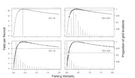
In order to disaggregate the effects of spatial heterogeneity in effort and on life history parameters, a simple simulation was developed depicting the effects of heterogeneity in fishing effort on Y/R where life history parameters are constant across the population. Spatial variability in F is assumed to follow a lognormal distribution and four simulation scenarios with CVs of 0, 0.5, 2 and 4.5 were considered. Lognormal distributions were used because they were able to describe the skewed nature of the data. For each scenario, 1000 random numbers with mean Fmax and specified CVs were drawn from this distribution, each representing the fishing mortality for 1/1000th of the recruits in the fishery. The realized Y/R was then predicted for each location within each scenario and the mean Y/R was calculated by averaging over all locations.

2.2.4 Com posite Y/R m odel

To develop a single model that reflects the variation in Y/R resulting from both heterogeneity in life history parameters and fishing effort, site-specific Y/R models based on local life history conditions were combined with historical effort patterns into a composite model. The steps that follow are also given in Fig. 2.1. This model accounts for the differences in fishing mortality from one location to another by allowing F to vary spatially.

As with a traditional Y/R analysis (Eqn. 2.1), Y/R for each location was computed for a range of fishing mortalities. Location-specific Fs were derived from the VMS data as given above. In the

composite scenario each overall F represents a mean across the fished area, and the location-specific Fs are adjusted linearly according to Eqn. 2.4 depending on the desired mean F. As the mean fishing mortality increases, the relative spatial distribution of fishing mortality remains the same but is scaled by a constant to reflect that overall mean. The relative distribution of location-specific Fs was generated using the median distribution of VMS fishing effort from 2007 to 2009. To derive the location-specific values that correspond to each mean F, the original F estimates are adjusted by a constant, C, that corresponds to each level of mean fishing m ortality f

(2.5) where

n

represents a location and fnmed the original median F at that site. The adjustment

Cf,

can then be isolated

(2.6)

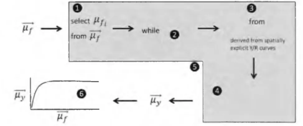
Figure 2.1: Development of the composite Y/R model. Steps are: (1) an average F, μfi , is selected from the vector of average fishing mortalities μ

f;

(2) fishing mortalities by location (f ) are derived from the observed fishing mortalities by location (fmed), scaled by Cf so that their mean is μfi

,

(3) the

Y

corresponding Y/R (-) are found for each location, using the spatially explicit Y/R curves; (4) the landings

(L)

weighted mean (μyi.) by location (n) of all expected Y/Rs is calculated; (5) The process within the gray area is repeated for all (6)

p.f

and μ

y

are combined to form the composite Y/R curve.

and since μ is a series of mean fishing mortalities and each

F nmed

is known, the adjustment that results in each mean F can be found. For each sequential mean fishing mortality,

F med

is multiplied by

Cf

to produce a vector of fishing mortalities for each particular mean. The final step in constructing the expected Y/R for each mean F is to find the average Y/R from the location-specific curves that

accompany

F med.

Here we use the Y/R averaged over all locations, but weighted the median landings by location from 2005 to 2009. The weighting increases the importance of those areas that have the most scallops. See Fig. 2.2 for an illustration of arriving at an expected Y/R based on a mean F.

For comparison, a similar procedure is followed to generate an optimal Y/R curve. The

difference is that the location-specific Fmaxs are substituted for

F nmed

so each location is fished at a rate relative to its optimum rather than relative to the observed effort. In this case there is an average fishing mortality that will result in each location being fished at Fmax. For the yield estimates from the uniform fishing mortality scenarios, a single F was applied to each location.

Fishing Mortality

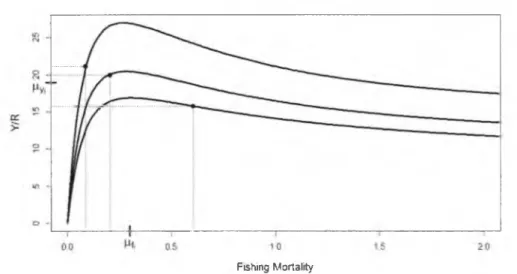
Figure 2.2: Example of the process for deriving the composite Y/R μy i on the plot) for a single value of average F μ

f i

on the plot). Spatially explicit values for F (dotted vertical lines) are matched with their corresponding Y/R curves and each expected Y/R is found (dotted horizontal lines). The Y/R are then averaged to get μ yi

.

This process is repeated for a sequence of increasing average fishing mortalities (μ f i resulting in vectors μf an d μy which make up the composite curve.

In addition, two selectivity patterns were used. They represent changes in fishing regulations (most importantly the size of the rings on the scallop dredges increased from 7.6 to 10.2 cm between the years 1994 and 2004). Selectivity follows a logistic distribution and is defined as

(2.7) where 0, is the selectivity at length

I,

and

a

and

b

are logistic equation parameters. The values of

a

for the current and historical selectivity periods, respectively, are 15.50 and 19.85 and for

b

are 0.14 and 0.24.

All analyses were implemented using R statistical software (R core team 2012).

2.3 Results

The simulation with varying CVs demonstrates that if not all locations are fished at optimal fishing mortality (Fmax) the maximum overall Y/R cannot be met because any departure from Fmax results in lost Y/R. Maximum Y/R was obtained only when the CV of the random lognormal numbers

approached zero, ensuring fishing mortality at all locations was Fmax. As the CV increased there was more departure from the mean and so more variability in Y/R by location (Fig. 2.3). Each trial distribution was centered on Fmax however, so even when the CV was high the average F was always close to Fmax.

Fishing Mortality

Figure 2.3: Yield per recruit curves with simulated distributions of F, assuming the average F is Fmax. Each distribution has a mean of 0.3 (Fmax) but the CVs vary as noted. The dashed line indicates the mean Y/R, which decreases as the CV increases.

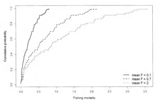
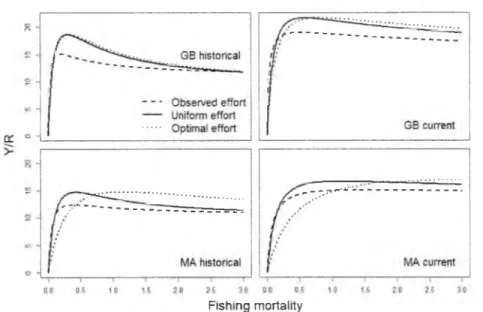
The composite Y/R model attempts to account for the variability in both effort and habitat. Each average F in this model corresponds to a distribution of location-specific Fs (Fig. 2.4) that are then linked to their location-specific Y/R curves (as in Fig 2.4). The shape of the composite Y/R curves (Fig. 2.5) depends on the selectivity and growth patterns, but some patterns are consistent among all

scenarios. The composite model results in less Y/R over most fishing mortalities than the uniform model that is typically employed by fisheries scientists. Secondly, the optimal Y/R model peaks at a higher fishing mortality than either of the other models especially in the mid-Atlantic. While some realizations of heterogeneous fishing effort (e.g., the optimal curve) can result in high Y/R, this case is not observed for either Georges Bank or the mid-Atlantic in the actual effort data.

A comparison of the selectivity patterns shows that the change in this function impacts the shape of the uniform and optimal curves but does not alter the composite curves as much. The historical selectivity causes a more notable decline in the uniform Y/R especially, because with smaller rings, high effort causes more loss in potential Y/R since more scallops are caught before they reach a large size.

Fishing mortality

Figure 2.4: Example of cumulative probabilities of spatial fishing mortalities at three observed average Fs.

2.4 D iscussion

The primary paradigm of fishery science and management has been to identify the stock-wide optimal fishing mortality and set effort levels to match this rate. The spatial distribution of effort has generally been neglected or ignored (Caddy 1975; Orensanz and Jamieson 1998; Caddy 1999). In the case of sea scallops with the observed spatial effort patterns, Y/R varies only slightly over a wide range of stock-wide fishing mortalities; it is often more affected by spatial effort patterns (Fig. 2.5). Thus, adjusting the spatial distribution of fishing mortality is more important here to optimizing Y/R (given the observed effort distribution) than changing the mean fishing mortality.

Harvest yield per individual for sedentary species is a function of both the local environment which affects the resource condition and the cumulative intensity of local fishing effort. Understanding these processes is critical for developing accurate predictions of Y/R. In the case of scallops in this region, shallower depths usually improve individual condition,

Fishing mortality

Figure 2.5: Y/R models assuming effort is distributed following the observed pattern, uniformly, and optimally on Georges Bank and in the mid-Atlantic under the historical and current selectivity patterns. The models based on the observed distribution of effort consistently give a lower Y/R than the uniform case.

probably because of higher availability of food (MacDonald and Thompson 1985; Hart and Chute 2009; Hennen and Hart 2012). Scallop fishermen, especially in the Mid-Atlantic, focus effort at particular depths (Fig. 2.6) to take advantage of this better condition; thus there is an individual incentive to fish these areas the hardest, even though the fishing mortality that optimizes Y/R at these locations is lower than in less productive areas.

The Atlantic sea scallop fishery provides a good model to demonstrate the relationship between fishing effort, Ymax and expected Y/R. As scallops move so little, the spatially-specific F can be assumed to act only on particular groups of individuals and so the dynamic pool assumption is violated (Caddy 1975). It is clear from comparing the spatially-specific Fmaxs to the estimated Fs (Fig. 2.6) that the behavior of fishermen is governed by rules other than those that maximize overall Y/R, resulting in suboptimal yield. While these issues are likely to be more pronounced in sedentary species, they will exist in any population where the probability of capture for individuals is not consistent. Equal probability of capture is in most cases unlikely (Paloheimo and Dickie 1964) and therefore some allowance for this heterogeneity is necessary to accurately predict Y/R.

Depth

Figure 2.6: Estimated location-specific fishing mortalities in the mid-Atlantic versus depth. The dashed line is a loess smoother through the data. The solid line represents the change in Fmax with depth, as estimated by Y/R models. The highest observed effort occurs at a depth of approximately 60 meters, though the theoretical highest effort should be at the deepest depths. A similar trend is evident on Georges Bank. Some estimated rates of fishing mortality are unrealistically high and this graph is cut off at F = 5, but the loess smoother uses all the data.

Each estimated Y/R in the composite model is a function of spatially specific environmental and harvesting conditions. The average Fs correspond to a set of local fishing mortalities, as well as location- specific Y/R curves (Fig. 2.2). The result is a model that averages lower Y/R than that predicted by conventional theory, in which each location is fished at the same rate. The Y/R is not lowered randomly because fishing effort is directed at certain areas. Interestingly, over much of the depth gradient in the Mid-Atlantic, fishing occurs where Y/R theory suggests there should be little, and vice-versa. At depths greater than about 60 m, observed fishing effort decreases while Fmax increases (Fig. 2.6). Thus the observed rates of fishing are high where Y/R suggests they should be low, and low where Y/R suggests them to be high. Such behavior results in the reduced overall expected Y/R seen in Fig. 2.5.

The effects on Y/R of spatial heterogeneity in both fishing effort and local environmental conditions have been investigated in the past. Hart (2001) showed how variability in fishing mortality, but with constant life history parameters, will result in Y/R that differs from that estimated by theory (as in Fig. 2.3). Smith (2001) looked at environmental effects on scallop growth and found depth to affect Y/R curves and subsequently the estimates for related reference points. An analysis of abalone in New Zealand had a similar finding, resulting in distinct Y/R curves for headlands and for bays (McShane and Naylor 1995). Fogarty and Murawski (1986) evaluated spatial effects on Y/R for surfclams, assuming density-dependent growth and an ideal free distribution of fishing mortality; i.e., F was directly

proportional to location-specific density. Even though their assumptions differed considerably from the work presented here, they also found the spatial effort distribution to considerably affect Y/R.

In order to make predictions of F and thus expected Y/R, a linear relationship between F and effort was assumed. While this is often a good approximation, it does not describe all situations (Addison and Bannister 1998). However, even if the relationship between fishing effort and F is

nonlinear, there would still be considerable variability in fishing effort, and it would be unlikely that all locations would be fished at an optimal rate.

The composite Y/R model implicitly assumes that the fishery will maintain the same spatial patterns of fishing effort, growth and natural mortality, as well as the relative distribution of landings (used in the weighted averaging). Effort patterns will change directly as a function of recruitment to the fishery and other natural processes as well as changes in management, such as the opening of access areas (as in Fig. 4.2). Changes in the distribution of effort alter the Fs on the location-specific Y/R curves, so the uncertainty in the Y/R estimates is directly linked to the effort distribution. However, suboptimal distributions of effort would be expected in the absence of rigorous spatial management regardless of these shifts.

While Y/R is often not used to set reference points because it neglects spawner-recruit effects, it is nonetheless an important description of fishery yield. Moreover, the dynamic pool assumption of spatial uniformity in effort is not unique to Y/R, and is assumed in most stock assessment models (Caddy, 1975; Orensanz and Jamieson, 1998), so similar discrepancies can arise with other assessment methods.

It has been demonstrated here that there can be substantial mismatches between actual, uniform, and optimal effort distributions that in turn can cause losses in Y/R relative to the Y/R

calculated assuming a dynamic pool. Such spatial effects need to be taken into account by scientists and managers in order to make accurate assessments and to optimize fishery yield.

3 Extending effort hetero g en eity to m ore com plex m odels

3.1 Introduction

The previous section gave evidence for how an unequal probability of capture for all individuals confounded expectations of Y/R. While that exercise is useful in demonstrating the concept, especially since Y/R is a simple model, it does not have a direct application to the scallop fishery; currently, the scallop resource is assessed using a catch-at-size assessment (CASA) model (Sullivan et al. 1990; NEFSC 2010). The model differs from Y/R in many ways, but most obviously it uses much more data and is able to estimate historical fishing mortality, recruitment, abundance, etc. It is size-structured, meaning the population dynamics act on groups of scallops organized into length bins. It is fit using maximum likelihood to indices from dredge surveys from 1975 to the present (Serchuk et al. 1979), video surveys from 2003 to the present (Stokesbury 2002) and 2012 to the present (Gallager et al. 2010) and also uses fishery-dependent landings and shell height frequency data.

While the CASA model is flexible and adaptable, it (like most stock assessment models) makes no explicit allowance for spatial heterogeneities in either the resource or fishing effort. Spatial heterogeneity in the resource began to intensify after 1994 when biomass started to increase dramatically in the closed areas (Hart and Rago 2006). The CASA model can make some attempt to account for the buildup of large scallops in closed areas by using a dome-shaped selectivity pattern (Hart et al. 2013) which reduces the expected catch of larger scallops, but this still does not begin to

Hart et al. (2013) examined the fit of the CASA model to simulated data and compared a whole- stock assessment to separate models run on open and closed areas. They found that splitting the stock spatially allowed the CASA model to perform better, probably because the domed selectivity is not flexible enough to represent the entire stock in aggregate, so the split model was more efficient.

Even though such a split model does much to ease the tension between the various survey indices, landings and size frequency distributions, there is still a great amount of spatial heterogeneity that remains unaccounted for. The goal of this section is to examine the influence of spatial

heterogeneity, especially in fishing mortality, on the accuracy of the stock assessment model and to offer a realistic description of the potential error inherent in ignoring the spatial distribution of fishing effort.

3.2 M ethods

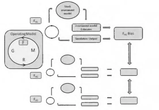
The methodology for this section can be separated into two distinct parts: (1) the fishery simulation operating model and (2) the stock assessment model. A functioning, realistic population and fishery simulation for sea scallops has been compiled where the spatial distribution of fishing effort can follow different assumptions regarding its degree of heterogeneity and the relationship between fishing effort and biomass. The simulation can then be used to evaluate bias in the scallop stock assessment model (CASA) as a function of these assumptions. Different characterizations of fishing effort are used in the stock simulations, and the model results are compared to the known simulated population statistics so that the consequences of heterogeneity in fishing effort can be quantified (Fig. 3.1).

Figure 3.1: General framework for the study in section 3.3. The operating model is repeated at differing levels of heterogeneity in fishing mortality and those outputs are used as inputs into the stock

bias at a particular level of heterogeneity in F, and the bias can be compared among the levels of heterogeneity. This framework is repeated under the random, ideal free distribution and weighted ideal free distribution scenarios.

3.2.1 The CASA m odel

Unless otherwise referenced, the following information can be found in appendix B11 of the 2010 sea scallop stock assessment,

Technical documentation for the CASA length structured stock

assessment model

(Jacobson 2010). The reader is referred to this document for a more detailed description of the population dynamic model and fitting procedure.

CASA is an entirely length-structured, forward simulating stock assessment model that estimates parameters using maximum likelihood. The length bins include a plus group that contains the

individuals greater than or equal to an externally estimated

L

∞, for the population. Time steps are yearly, in accordance with catch statistics and survey periods, and as such all instantaneous rates assume a one year period. Parameters such as fishing mortality or recruitment are estimated as deviates from a geometric mean. For example, recruitment in year

y (Ry )

is calculated as

3.1 where

p

is the model estimated geometric mean recruitment and

yy

is the estimated deviate for year

y.

This assumes the deviation from mean recruitment to be lognormally distributed.

Growth occurs at the beginning of the year and is implemented using growth transition

matrices. The matrices may be derived internally using supplied growth increment data or they may be input directly. Recruitment occurs after growth. Scallops mostly spawn synchronously, likely cued by temperature or tides. In different areas they may spawn (and thus recruitment may occur) at different times, likely depending on environmental cues (MacDonald and Thompson 1988), and there is also evidence of multiple spawning events per year in some places (DuPaul et al. 1989) as well as protracted spawning (Langton et al. 1987). Given these timing differences, as well as individual differences in growth rates (Hart and Chute 2009), it is likely inaccurate to assume that recruits enter a single bin at the start of each year. The CASA model accounts for this by using a Beta distribution (fixed over years) to estimate the proportion of recruits that enter each size class.

Natural mortality can vary by year as well as by length, but in this study it is fixed across both. Incidental mortality, which is mortality caused by the fishing gear but separate from discard mortality is proportional to fishing mortality and may also vary by size, but is not employed here. Mortality rates are derived using the catch equation, where catch is the sum of landings and estimated discards. Fishery selectivity may take a variety of forms including a double logistic (dome shape) that is useful when some of the stock is inaccessible to the fishery, as is the case with the Georges Bank closures.

The objective function value is the weighted sum of all the negative log likelihoods for the data in the model. The likelihoods can come from various assumed distributions depending on the type of data (e.g., Gaussian for catch weight; multinomial for survey length compositions, etc.).

Many options, such as discard mortality, incidental mortality, or estimation of survey and fishery selectivity parameters are unused in this simulation because they are not necessary for answering the spatial questions proposed here, and would only increase the complexity of the results.

3.2.2 Data

The simulation relies heavily on data from the annual NMFS scallop survey; brief survey

methods are outlined here using information from NOAA (2013). This survey has run continuously since 1977. For 30 years it was carried out on the NOAA vessel Albatross IV, but switched in 2008 to the R/V Hugh R. Sharp out of Lewes, DE. Calibrations were performed to ensure consistency in the data. The survey uses a 2.4 m New Bedford style scallop dredge with 51 mm rings with a 38 mm liner inside. Each tow lasts 15 minutes at a speed of about 7 km/h, covering a distance of approximately 1.8 km. Sensors on the dredge provide diagnostics that assess the efficiency of the tow by taking measurements of pitch, roll and depth.

The survey has typically run in June and July. Historically approximately 450 dredge stations were sampled, but since 2011 the HABCAM towed camera system (Gallager et al. 2010) has been integrated into the survey design and at present about 200 dredge stations are sampled. The survey follows a stratified random design where the strata are the shellfish strata used for all NEFSC shellfish surveys (Mohn and Roddick 1987). The strata are based on area and depth.

After scallops are brought on deck by the dredge sampling commences. When possible all scallops are measured and weighed, but when catch rates are very high the catch is subsampled. Meat and gonad weight samples are taken from some of the catch, and scallop shells are kept for age analysis. Other measurements regarding the bottom type and animal community, temperature, salinity and phytoplankton concentrations are also taken.

3.2.3 Fishery Sim ulation

The fishery simulation that serves as the operating model in this study is spatially flexible in growth, recruitment and fishing mortality. Each of these processes can be isolated in order to evaluate the model's response to the heterogeneity they create, or they can be allowed to vary spatially

together, approximating the most realistic scenario.

As in the CASA model, the operating model is structured by size rather than age. The length bin midpoints range from 47.5 to 142.5 mm in increments of 5. The last bin in the CASA model is typically used as a plus group (Jacobson 2010); however, scallops in the simulation do not grow larger than the maximum size for the growth transition matrix so in this case the last CASA bin is not a plus group.

Natural mortality does not vary in this simulation. A method for estimating M that uses the decomposition rate of the shell hinge is available (Dickie 1955; Merril and Posgay 1964; NEFSC 2010), but there is little published information that applies this method. Further, the rates of hinge

decomposition on Georges Bank have been found to depend on environmental conditions (Merril and Posgay 1964), so this variability would have to be accounted for. M has also been estimated directly, but on a very small scale (e.g., MacDonald and Thompson 1986). Given the limited understanding of natural mortality even on a broad scale, the simulation did not allow for variability in this parameter. In addition, it is not critical for answering the questions that this simulation addresses. M is assumed at 0.12 for Georges Bank, as in NMFS stock assessments (NEFSC 2010). The other three population dynamic rates, growth, recruitment and fishing mortality (no immigration or emigration is necessary for scallops) are explained below in subsequent sections.

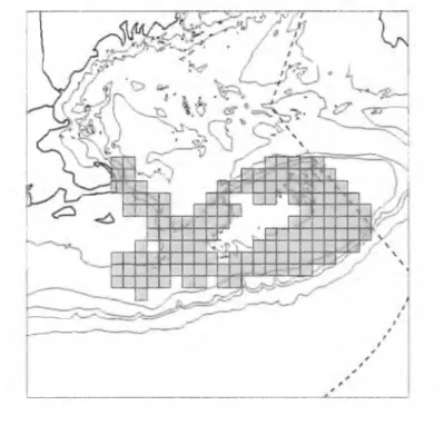
The simulation uses the spatial orientation and bathymetry of Georges Bank. A grid comprised of 10x10 minute squares (following convention, e.g., Premetz and Snow 1953) is overlain across the area (Fig. 3.2). The entirety of Georges Bank is not covered, most notably the shallows in the middle section. Scallops are uncommon in that area, so the annual survey does not make tows there.

Figure 3.2: The Georges Bank spatial grid used in section 3.3.

Observation error in some input data into the CASA model is not considered in this study so that uncertainty in the results can be focused on the consequences of spatial heterogeneity in fishing effort. The survey index is a perfect representation of abundance because all locations are sampled and the survey sampling efficiency is 1 for all size classes. In the same vein the fishery length frequencies, which are typically derived from sampling less than 10% of scallop trips, are again perfectly represented. Fishery selectivity is fixed and logistic in shape, and is input directly into the CASA model (i.e., it is not estimated). The R code used for this simulation can be found in Appendix A.

3.2.3.1 Order of o peratio ns in the sim ulation

Given the structure of the submodels, the population dynamics cannot be modeled

continuously. This is the most unrealistic for the growth submodel. While growth is well-studied, it is modeled using annual growth increments (Merrill et al. 1966; Hart and Chute 2009). It is possible to determine the seasonal cycle in growth using oxygen isotope samples between increments because the isotopes are a proxy for temperature (Krantz et al. 1984; Tan and Roddick 1988; Chute et al. 2012). However, isotopic analyses are expensive and time consuming so sample sizes for these studies are small; as such it may not be accurate to apply the seasonal patterns to the entire population. Another possibility could be to model high resolution growth patterns using a tagging study (e.g., Harris and Stokesbury 2006), but again much sampling effort would be required. Given the lack of information on

Spawning on Georges Bank typically occurs in fall (Posgay and Norman 1958), although there is evidence for a spring spawn as well (Dibbacco et al. 1995). The mid-Atlantic incurs a semiannual spawning cycle (DuPaul et al. 1989). While it is certain that spawning occurs two times per year in both these regions, the relative sizes of the spawning events in any given year are unknown and likely vary from year to year. Due to this lack of information, only a single spawning event is used in the model.

While growth and recruitment are modeled as discrete processes, mortalities are instantaneous rates integrated continuously over the entire year following growth and recruitment. They are

implemented using exponential decay equations, as is typical for fisheries models (e.g., Ricker 1975). These processes begin after growth and recruitment and so act on the updated numbers-at-age after the beginning of the year. Instantaneous rates make the simulation compatible with Baranov's catch equation, which is used to reconcile continuous harvest rates with the continuous rates of natural mortality.

3.2.3.2 G row th transition m atrix

To account for growth in the simulation, depth- and latitude-dependent growth transition matrices (Sullivan et al. 1990; Sullivan 1992; Chen et al. 2003) were developed corresponding to the mean depth and latitude of each 10x10 minute square. Growth transition matrices describe the probability that an individual in a particular size class will grow into another size class over a single time step. They are useful because they can characterize stochastic error that is not wedded to a particular error distribution and they are easily incorporated into this type of simulation. The growth transition matrix has the form

P1,1 P1,c P1,C

G = Pi,c Pi,c Pi,C

0 0

Pc,c

(3.2)

where the rows represent starting size classes and the columns the size classes that are grown into.

G

is the growth transition matrix and p is the probability that a scallop in the size class belonging to row

i

will grow into the size class represented by column

c

and

C

is the total number of size classes. Scallops are assumed not to exhibit negative growth, so the entire lower left triangle of

G

is composed of zeros. If the number of scallops in each size class is given by the vector

N,

then the number of scallops at time step

Nt+1

is

The inverse of matrix G is used so that it multiplies appropriately with vector

Nt.

(3.3)

The transition matrices are not estimated directly from growth increment data. Instead they are built via simulation, using parameters from a von Bertalanffy growth model. Hart and Chute (2009) estimated parameters

K

and L

∞

, from the growth increment form of the Von Bertalanffy growth model (Fabens 1965; Quinn and Deriso 1999). The growth increment model is

where

L t

is the length of an individual at time

t

and AL is the change in length. This growth increment model can be combined with Von Bertalanffy's nonlinear equation to achieve a linear model which, as derived by Fabens (1965) is

(3.5) where At is the time step (always 1 here) and is the normally distributed error associated with individual

i.

Since multiple increments are read on each individual scallop, Hart and Chute (2009) also accounted for repeated measures by using a mixed effects model.

Hart and Chute's (2009) model estimated

K

and L

∞

on Georges Bank and in the mid Atlantic. Their model also included covariates latitude, depth and whether an area was open or closed to fishing because growth rates differ depending on local environmental conditions (MacDonald and Thompson 1985; Pilditch and Grant 1999). For the development of the simulation growth transition matrices, the model for Georges Bank open areas that includes depth was chosen because closed areas were not implemented in the simulation. Those parameters were estimated to be

K

= 0.574 — 0 .0 0 1 3 4 d (3.6)

and

L

∞

, = 177.4 — 0 .8 8 2 d (3 .7 )

where

d

is depth. These two parameters can be used in Eqn. 3.5 above, with At = 1 to approximate the growth increment. Using the growth increment formula makes the estimation of the third parameter from the classic von Bertalanffy model, t 0, impossible (Fabens 1965; Francis 1988) and it is assumed to be zero.

In the estimation process, mixed effects models also derive the correlation between the estimated parameters. Hart and Chute (2009) estimated the correlation between

K

and L ∞ after converting to the nonlinear form using a Taylor series to account for the change in variables. They found these variables to be positively correlated at approximately

p =

0.65. This correlation is used together with estimates for the mean and standard deviation of the parameters to derive the growth transition matrix.

Monte Carlo simulation (Metropolis and Ulam 1949) is used to develop the spatially-referenced growth transition matrices.

K

and

L

∞ are assumed to come from a multivariate normal distribution

Where μ is a vector of means

(3.8)

and ∑ is the covariance matrix

(3.9)

(3 .1 0 ) and σ2 is the variance of

K

or

L

∞ and

co v()

is the covariance function. The variances came directly from Hart and Chute (2009). The covariance was calculated according to the formula

where σ represents the standard deviation of

K

or

L∞

and the correlation is p (0.65).

(3.11)

Using the means, standard deviations and correlation, random multivariate normal numbers were generated using R's MSBVAR package (Brandt 2012). Three thousand correlated random numbers were generated per 5 mm size class, representing simulated values of

K

and for individual scallops. Each scallop's starting size

L t

was assigned randomly within the 5 mm bin. For each of the 3000 scallops per size class, growth then occurs according to Eqn. 3.5, using the

K

and

L

parameters from the

∞

multivariate normal distribution in Eqn. 3.8. The results are tabulated in a matrix of counts that represent the occurrence of growing from each starting size bin to the potential ending size bins. That matrix is then converted to proportions.

The process is complicated in the larger size classes. represents an average maximum size for a population; this means that each individual has a specific maximum size that may be larger or smaller than the population

L∞

.

This uncertainty is modeled using the Monte Carlo method described above. However, in the larger size classes the random draws for the starting size may be larger than

L∞

.

In these cases equation (3.5) will predict negative growth and those draws must be rejected. One solution is to make the bin containing

L∞

the terminal bin, but the approach taken here is simply to use rejection where the assigned length of an individual is greater than its assigned

L∞

.

Figure 3.3: Recruitment on Georges Bank in 2009. Spatial autocorrelation is apparent, with large recruitment events in the Great South Channel and on the Northern Edge.

3 .2.3.3 Recruitm ent

A modeled spatial distribution of sea scallop recruitment should be patchy in nature (Caddy and Seijo 1998), as is observed in the data (Fig. 3.3). As such, it is important to replicate the type of spatial correlations observed in nature within the recruitment submodel. Since the simulated scallops are stationary, the spatial coherence at the recruitment stage is important in determining the spatial coherence at later stages.

One solution to incorporating spatial coherence into the recruitment distribution is to use correlated multivariate distributions. In this case a variance-covariance matrix for the entire region

(including all years and divided up into 10x10 minute squares) can be generated using all the available data. Then random correlated numbers can be drawn from a specified multivariate distribution that incorporates the observed covariance; in this manner the historical spatial coherence is respected. There are two problems with this method, however. The first is that it is not general. While there are almost 30 years of recruitment data, not all 10-minute squares are sampled in every year so the actual sample size for the covariance between two spatial units is always fewer than 30. Consequently, the potential for random error in the covariance resulting from small sample size is considerable. In addition, the specific covariance between any two spatial units is not of particular interest for these analyses. The second problem is that the large number of spatial units (81) make the simultaneous generation of random correlated numbers impossible on a personal computer.

A more general approach comes from using spatial statistics. The steps involved are: (1) estimation of yearly variogram parameters; (2) describing the parameters using distributions; (3) constructing variograms using randomly generated parameters from those distributions in (2); and (4) simulating recruitment. Each of these are discussed in turn.

The recruitment data used in this procedure are taken directly from the survey history. Survey recruits are defined as those individuals that are between 40 mm (the mesh size of the NMFS survey liner) and one year's growth of 40 mm.

Many spatial statistic approaches require the removal of the first-order trend so that the data are stationary, meaning that the statistical properties of the data (e.g., mean and variance) do not vary by location (Bailey and Gatrell 1995). Therefore, before the following analyses a linear model was fit to the data of the form

where r is the recruitment history,

x

is the x spatial location,

y

is the y spatial location,

d

is depth and the β parameters represent the coefficients for each term . A full saturated model including all interactions was used so that the first order trend in recruitment was close to the average first order trend.

3 .2 .3 .3.1 Estim ating yearly variogram s

Variograms indicate the semivariance of values belonging to a spatial data set at binned distances. The classic definition of a variogram is (Baily and Gatrell 1995)

where

y

is the semivariance,

h

is the separation distance between points (x axis in the variogram),

n (h

) is the number of point pairs within bin

h

and Si and

Sj

are values at given locations within bin

h.

The semivariances can then be plotted against distance in order to show how variability increases with distance. The typical expected structure for a variogram is increasing semivariance with increasing distance between point pairs, often with the semivariance reaching an asymptote.

Each of the classic variogram models can be described using three parameters: the sill, the nugget and the range (Fig. 3.4). The sill is the maximum modeled semivariance where the model asymptotes. The range is the distance between point pairs where the semivariance is equal to the sill

(3.12)

and the nugget is a minimum amount of semivariance between locations at a distance of

h

= 0. Theoretically a nugget should not exist but it typically does because of the relationship between sample variance and the spatial scale of the samples, or because of measurement error.

Figure 3.4: Example of a typical variogram. N is the nugget, R is the range and S is the sill.

Variograms are often used within a spatial interpolation method known as kriging, which is the basis for the final recruitment simulation method used here. There are different variations on kriging, but all are linear models where a value at a location can be predicted using a weighted sum of observed values. When a model is fit to an empirical variogram, the model serves as a way to populate a

covariance matrix with expected covariances for each pair of locations. The covariance matrix is combined with a distance matrix that measures the distance between each interpolation location and each sample location. The product of the inverted covariance matrix and the distance matrix gives the kriging weights that are used to estimate values at unobserved locations (Bailey and Gatrell 1995).

Any model may be fit to an observed sample variogram (e.g., linear would be the simplest), but classic variogram models are spherical, exponential and Gaussian (Bailey and Gatrell 1995). These three models are similar in that each increase until they reach an asymptote. The spherical model, the model used here to estimate the semivariance,

y,

for the scallop recruitment data, is written as (Bailey and

where, r is the range and σ2 is the sill. An example of a typical variogram is given in Fig. 3.4.

The spherical model is fit here using weighted least squares (Cressie 1985) with the R package "gstat" (Pebesma 2004). The variograms are fit using the residuals from Eqn. 3.12 which should be closer to stationary than the raw data. Thus the residuals used to fit the variogram are

Gatrell 1995)

(3.15)

3.2.3 .3 .2 Describing variogram p aram ete rs w ith distrib utions

Spherical models are fit to variograms for each of the years 1983-2009, giving 26 total parameter estimates for the nugget, range and sill. When taken together these three parameter distributions represent an approximation of the variability in spatial coherence from year to year. The simulation requires sill range and nugget values for each year in the simulation, so Gaussian

distributions are fit via maximum likelihood to each parameter set using R's MASS library (Venables and Ripley 2002). The covariance between each set is also estimated. Thus the sill, range and nugget can be represented by a multivariate normal distribution

V

(3.16) where

p

is a vector of means and E is the covariance matrix.

3.2.3 .3 .3 Constructing a sim u lation -year variogram

In any year of the simulation, the spatial distribution of recruits is derived from a variogram that is constructed from randomly generated sill, range and nugget parameters, given as

(3.17) where

gy

is the recruitment variogram parameters in year

y,

and

vn, vr

and

vs

are random, correlated numbers from the multivariate distribution described in Eqn. 3.8. As such, the shapes of the potential simulated variograms from

V

cover the range of historical spatial recruitment but are not limited to the actual observed values.

3 .2 .3.3 .4 Sim ulating and scaling recru itm en t

The final step is to use the simulation-year variogram to randomly generate a recruitment field. This is accomplished using R's gstat package (Pabesma 2004). While kriging models are deterministic, it is possible to use a similar process to generate stochastic simulations given the data and a specified variogram. In the Gaussian simulation method, used here, a random path is followed through the set of prediction locations. At each iteration (for each location) the distribution of potential values is

computed conditional on the data and locations that have already been simulated. A value is drawn from this distribution and added to the data set and this process is repeated until predictions have been made at all locations (Bivand et al. 2013). Since the value at each location is dependent on the

conditional distribution that will satisfy the parameters of the kriging model (variogram, mean etc.) the final map is an accurate representation of the inputs. Using the methods described here, the spatial coherence of recruitment is satisfied on a log scale rather than a real scale.

The randomly generated recruitment map is then scaled to provide the desired total

recruitment. Recruitment in year y,

R*y,

is the product of the recruitment estimated within the random field calculation

Ry

and a constant that will scale that recruitment such that

given that

where

Ry

is the vector of simulated recruitment,

hy

is a randomly drawn number from the recruitment history, and ωy is a constant that scales the values at each location so that they sum to the desired recruitment level

hy .

The

hy

are expanded directly from survey recruitment to the stock size, assuming a dredge efficiency of 0.4. This efficiency estimate is close to values assumed for the survey dredge in NMFS stock assessments, which has been estimated to lie between 0.36 and 0.43 (Jacobson et al. 2007). It is likely to be an underestimate for recruits because scallops of this size, while still larger than the dredge mesh size, are more active swimmers and probably more likely to evade the dredge on average. However, the purpose here was simply to scale recruitment to a reasonable level; the actual value need not be directly comparable to the stock size to achieve the goals of this simulation.

3 .2.3 .4 Fishing M ortality

The most critical component of the simulation is the implementation of fishing effort because the purpose of this study is to determine how the spatial distribution of fishing effort biases the CASA model. There are two aspects that determine the nature of fishing effort in the simulation: (1) the degree of heterogeneity in fishing mortality, and (2) how values of fishing mortality are assigned to each spatial location (Fig. 3.5). This allows for two approaches to examine how the violation of the equal probability of capture assumption may bias the model.

Figure 3.5: The scenarios describing how fishing mortality occurs. The different levels of heterogeneity are expressed through the exponent

v,

and each level of heterogeneity is crossed with each type of fishing mortality assignment.

In order to give sufficient contrast within the system so that the CASA model is able to more easily estimate parameters, the mean yearly fishing mortality starts low then increases and decreases again (Fig. 3.6). The observed fishing mortality within the simulation is not simply the fully selected F that determines this overall increase and decrease in fishing pressure (Fig. 3.6) unless under the uniform fishing mortality scenario (see section 3.2.3.4.1). In order to determine this statistic Baranov's catch

equation is solved for fully recruited fishing mortality

F

in year

y

by minimizing the least squares objective function

0

(3.20)

where

L c y

are the landings from size class

c

in year

y, Өc

is the selectivity for size class

c, Nc,y

is the population number in size class

c

in year

y

and

M

is natural mortality. Since there is no discarding in the simulation catch is equivalent to landings.

3.2 .3 .4.1 Describing hetero g en eity in Fishing m ortality

The distribution of fishing mortality comes from vessel monitoring system data. The median fishing effort by location from 2000 to 2009 is used as a baseline, and effort is assumed to be directly proportional to fishing mortality. The skew of the observed fishing effort

E

is adjusted by raising the observed

E

to a power,

v.

The skew-adjusted fishing effort

E

* under a particular variance scenario is

where

v

is a number > 0 that alters the heterogeneity in fishing effort. Numbers between zero and one reduce the skew relative to the baseline distribution, while numbers greater than one increase the skew. A uniform distribution of fishing effort is achieved when

v

= 0. Within the simulation, the effort is converted to an average fishing mortality, so the

E*

is adjusted to achieve the desired average F. A constant given a particular desired mean fishing mortality in year

y (Ey ), λ y,

is derived so that the product of the constant and

E*

will achieve the desired mean F,

F.

The equation for the mean scaled by a constant is

and the constant necessary to reach the desired mean can be isolated

where

N

is the number of observed fishing mortalities and

Fi*

represents the fishing mortality at location

i.

Effort is converted directly to fishing mortality because they are assumed to be proportional. The final F applied to each location is then

(3.21)

(3.22)

The

F

y,i are then matched up with fishing locations.

(3.24) (3.23)

Model Year

Figure 3.6: Theoretical fully selected fishing mortality over the model period. This pattern holds when the capture probability for all individuals is equal, but differs from the observed fishing mortality when this assumption is not met.

3.2.3 .4 .2 Assigning Fishing m ortality to locations

Thus far values of fishing mortality appropriate to the particular heterogeneity scenario have been defined. The next step is to assign those values to locations. Three assumptions are available to describe the distribution of fishing effort: (1) random; (2) assuming an ideal free distribution (IDF; fishing mortality by location is in proportion to the location's biomass); and (3) assuming a weighted ideal free distribution (WIDF; the fleet is prone to fish on biomass, but weighted by distance to shore). The IDF scenario was similar to the approach taken by Caddy (1975) in his simulation of scallops on Georges Bank and that of Fogarty and Murawski (1986) in their model of the surf clam fishery. Each of the three scenarios is crossed with all the values of skew considered (Fig. 3.5).

In the random scenario values of fishing mortality are assigned to spatial locations in no order. In the IDF scenario, biomass by location is ranked, and fishing mortality sequentially assigned so that the highest F occurs where the biomass is highest. For the WIDF scenario, biomass is multiplied by a weighting according to (the complement of) the location's distance to shore; fishing mortality is then assigned according to the weighted order.

3.2.3.5 Population dynam ic eq uations

Combining these submodels, the population dynamics for one simulation year can be described by the following steps:

(1) Growth

(3.25)

(3) Mortality

(3.26)

where

Nt+G

is the population abundance after growth,

Nt+G+R

is the population abundance after recruitment (both growth and recruitment occur instantaneously), and

Nt+1

is the population abundance at the end of the year. Total landings

L

in number are calculated using Baranov's catch equation as

(3.27)

(3.28)

3 .2.3.6 Sim ulation output and CASA runs

The simulation outputs that are required for the CASA model are total landings, fishery-

dependent length compositions and total survey abundance and length composition. These will vary by simulation run and scenario. Other parameters, such as growth transition matrices, shell height to meat weight relationships and CVs associated with estimates do not vary with each run. See Appendix B for the input parameters to CASA. R compiles all the necessary input files and then runs the executable for the CASA model. CASA model outputs are read back into R so that comparisons can be made between the simulation's "true" values and the CASA model estimates. In order to focus the analyses on the result of interest, the effects of spatial heterogeneity on stock assessment, growth was assumed constant across the stock. Recruitment was allowed to vary spatially however because this was more directly related to the fishable population abundance which drives the simulation.

Error in the CASA model is described using a proportion bias

(PB),

which is

(3.29) where y is a (yearly) estimate from the CASA model (landings, fishing mortality, etc.) and y is the actual observation. Since y is subtracted from y , if the CASA model is overestimating a quanitity

PB

is positive and if CASA is underestimating

PB

is negative. The simulation is repeated 200 times for each crossed scenario, so PB is based on a large pool of estimates.

3.3 Results

3.3.1 G row th

Growth transition matrices were developed to allow individuals to grow instantaneously at the beginning of each year in the simulation. As described in the methodology section, due to the nature of the algorithm some growth increments had to be rejected because the randomly assigned to the scallop was smaller than their assigned size within the bin. Predictably, the probability of rejection grew

as the scallops increased in size (Fig. 3.7). The maximum proportion rejected, however, was approximately 0.6 meaning that (given the 3000 simulated individuals per size class) the minimum sample size upon which any transition-at-size was based was still 1200.

Shell Height

Figure 3.7: Probability of rejection in the simulation used to develop the growth transition matrix. Rejection occurs when the

L∞

assigned to a scallop is smaller than its actual size.

Scallops within the simulation grow according to the typical model where growth slows as individuals age. This is evidenced by consecutive size class distributions before and after growth (Fig. 3.8). Peaks in the size frequency are transposed farther when they begin at a smaller shell height than they do when they begin at a larger shell height.

60 80 100 120 140

Shell Height (mm)

Figure 3.8: Four examples of length composition in year t (solid line) and in the subsequent year t+1 (dashed line). No mortality is included.

3.3.2 Recruitm ent

One of the goals of the recruitment simulation was to preserve the observed spatial coherence as well as its variability. A range of potential spatial relationships (i.e., variograms) were developed using the data. The model randomly selected a variogram to use for each simulation year and in some years the spatial coherenc