Image Reconstruction and Enhanced Resolution
Imaging from Irregular Samples
David S. Early, Member, IEEE, and David G. Long, Senior Member, IEEE
Abstract—While high resolution, regularly gridded
observa-tions are generally preferred in remote sensing, actual observaobserva-tions are often not evenly sampled and have lower-than-desired res-olution. Hence, there is an interest in resolution enhancement and image reconstruction. This paper discusses a general theory and techniques for image reconstruction and creating enhanced resolution images from irregularly sampled data. Using irregular sampling theory, we consider how the frequency content in aperture function-attenuated sidelobes can be recovered from oversampled data using reconstruction techniques, thus taking advantage of the high frequency content of measurements made with nonideal aperture filters. We show that with minor modifica-tion, the algebraic reconstruction technique (ART) is functionally equivalent to Grochenig’s irregular sampling reconstruction al-gorithm. Using simple Monte Carlo simulations, we compare and contrast the performance of additive ART, multiplicative ART, and the scatterometer image reconstruction (SIR) (a derivative of multiplicative ART) algorithms with and without noise. The reconstruction theory and techniques have applications with a variety of sensors and can enable enhanced resolution image production from many nonimaging sensors. The technique is illustrated with ERS-2 and SeaWinds scatterometer data.
Index Terms—Irregular samples, reconstruction, resolution
en-hancement, sampling.
I. INTRODUCTION
I
N TYPICAL microwave remote sensing applications, observations of the surface properties are made with a sampled aperture approach in which the measurements are spatially filtered surface data sampled over a two-dimensional (2-D) grid. The aperture function is defined by the antenna pattern and/or signal processing techniques used to resolve the antenna illumination pattern into smaller spatial elements. Spatial sampling is typically obtained via pulsed operation and antenna scanning. The resulting measurements are often on an irregular grid and may have spatially varying aperture function responses. At times, the sensor may not even be considered an “imaging sensor” since the aperture filtered samples do not completely cover the surface. Nevertheless, we desire to generate the highest possible resolution images to aid in understanding geophysical phenomena.Gridded images can be generated with the “drop-in-the-bucket” techniques by assigning each measurement to a grid element in which its center falls. However, the resolution of such images is limited by the aperture response and for
Manuscript received January 10, 2000; revised June 5, 2000. D. S. Early is with @link Networks, Lousville, CO 80027 USA.
D. G. Long is with the Electrical and Computer Engineering Department, Brigham Young University, Provo, UT 84602 USA (e-mail: [email protected]).
Publisher Item Identifier S 0196-2892(01)01168-8.
many applications higher resolution is desired, leading to interest in image reconstruction and resolution enhancement algorithms. Under suitable circumstances, such algorithms can provide improved resolution images by taking advantage of oversampling and the response characteristics of the aperture function to reconstruct the underlying surface function sampled by the sensor. When single-pass sampling is inadequate, it may be possible to suitably modify the sampling by com-bining multiple observation passes to improve the sampling density, resulting in oversampled observations. In application, reconstruction/resolution enhancement algorithms can generate images from the observations at a resolution better than the mainlobe aperture resolution of the sensor.
In this paper, a tutorial approach is used to present and dis-cuss fundamental theories for image reconstruction and reso-lution enhancement from noisy irregular samples based on al-gebraic reconstruction techniques. While motivated by use in microwave remote sensing, the general theory applies to a va-riety of other sensors. In Section II, the theory of image recon-struction from irregular samples is considered. In Section III, we show the equivalence of the algebraic reconstruction technique (ART) [6], [7] and the irregular sampling/reconstruction theory discussed in the first section. Using simulation, we demonstrate that reconstruction can recover sidelobe information and con-sider the practical use of the theory in the presence of noise in Section IV. We compare the performance of additive and mul-tiplicative ART algorithms with the scatterometer image recon-struction (SIR) algorithm, a row-normalized derivative of mul-tiplicative ART tailored to reduce the influence of noise on en-hanced resolution image reconstruction [1], [2]. We discuss the effects of the aperture function on the resolution enhancement, concluding that for a fixed aperture area, an elongated aper-ture with varying orientation can provide the best resolution enhancement capability, depending on the sampling density. In Section V, the utility of the technique is demonstrated using ac-tual data. This introduction is concluded with a brief presenta-tion of the system model used in this paper and a comparison of traditional uniform sampling/reconstruction and irregular sam-pling/reconstruction.
A. System Model
Let represent the true surface image at a point ( ). The measurement system can be modeled by
noise (1)
where is an operator that models the measurement system (sample spacing and aperture filtering), and represents the ob-servations or measurements made by the instrument sensor. The 0196–2892/01$10.00 © 2001 IEEE
set of measurements are a discrete sampling of convolved with the aperture function (which may be different for each mea-surement) with a particular measurement written as
noise (2)
where is the aperture response of the th measurement. For image reconstruction or resolution enhancement, we are interested in the inverse problem
(3) where is the estimate of derived from the measurements . The inverse of the operator , , is exact only if is invertible and the measurements are noise free, in which case,
.
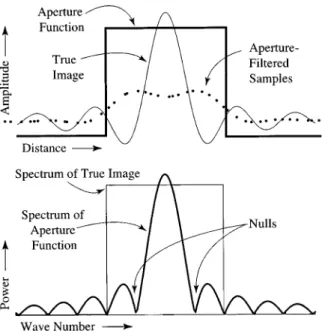
For a fixed aperture function, aperture-sampled data is equiv-alent to ideal sampling of the image function convolved with the aperture function (which is also termed a point-spread func-tion), which typically has low pass characteristics. The effects of the aperture function are twofold. First, various frequencies, particularly in the sidelobes, are attenuated. Second, the aper-ture function may have nulls in its spectrum. While nulls can lead to irretrievable loss of information, if the sampling density is sufficiently high, data from even very low sidelobe levels can be recovered with an appropriate algorithm. This is true even when irregular sampling and variable aperture functions are in-volved.
Compared to traditional (uniform sampling) reconstruction, this irregular sampling reconstruction can be considered a form of resolution enhancement since high frequency information suppressed (but not nulled out) by the aperture function is re-covered. We note that if there is noise in the system, a tradeoff between the resolution enhancement and the noise level exists since high frequency noise tends to be amplified in the recon-struction process.
B. Sampling and Reconstruction
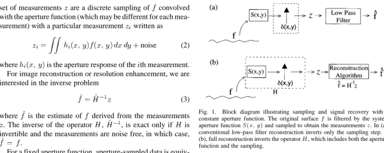
The traditional approach to sampling and reconstruction is founded on uniform sampling and the well known Nyquist sam-pling theorem [3]. Based on the Nyquist theorem, a bandlimited function can be completely reconstructed from regularly spaced samples if the sample rate exceeds the Nyquist sample rate of twice the maximum frequency in the signal. In typical applica-tion, signal reconstruction is accomplished with only a low pass filter. In effect, the aperture function is treated as an ideal low pass filter with no sidelobes and is ignored in the reconstruc-tion [see Fig. 1(a)]. For this case, the recovered frequencies are deemed limited to the width of the main lobe of the frequency response of the aperture function. The aperture function also acts as a prefilter to minimize high frequency components of the signal that might otherwise cause aliasing in the reconstructed signal.
Real-world aperture functions, however, are nonideal and have sidelobes. The sidelobes still contain enough information to recover at least some of the higher frequency content of the original signal if the (possibly irregular) sampling is dense enough. This requires inverting both the effects of the aperture
Fig. 1. Block diagram illustrating sampling and signal recovery with a constant aperture function. The original surfacef is filtered by the system aperture functionS(x; y) and sampled to obtain the measurements z. In (a), conventional low-pass filter reconstruction inverts only the sampling step. In (b), full reconstruction inverts the operatorH, which includes both the aperture function and the sampling.
function and the sampling [see Fig. 1(b)]. The reconstruction compensates for the aperture filtering by amplifying attenu-ated frequencies, though the aperture function may limit the reconstruction due to nulls in its spectrum.
If the sampling is regular (uniform) with a fixed aperture function, the reconstruction can be accomplished with Wiener filtering, an inverse filtering technique that also accounts for noise in the measurements [3]. However, inverse filter methods are difficult to apply when the sample spacing is irregular or when aperture functions vary with different observations. To ad-dress these problems, the next section considers irregular sam-pling and reconstruction theory in greater detail. We address the variable aperture by the use of algebraic reconstruction, showing that it is applicable for reconstruction from irregular samples. We later demonstrate that suitable variation in the aperture func-tion can eliminate nulls in the reconstrucfunc-tion.
II. IRREGULARSAMPLINGTHEORY
While the theory of sampling and reconstruction is well known when the sampling is uniform, irregular sampling and reconstruction theory is less familiar. Irregular sampling problems have been examined since the early 1960s (see [4]). However, in most studies, restrictive requirements are placed on the irregular sampling grid. Alternately, an arbitrary irregular grid can be parameterized by , which describes the maximal spacing in the grid. This approach places no restrictions on the structure of the sampling grid and is preferred in this study because it is a more general model of satellite sampling grids, especially when multiple orbit passes are combined.
To consider the validity of reconstruction from such irregular samples, recent work by Karl Gröchenig [5] is discussed. In order to discuss the important lemmas and theorems, certain formal definitions and groundwork are first presented. These include definitions of the spaces and functionals used and some auxiliary information not presented in the cited text but which help clarify the development.
Let denote the Hilbert space of square-integrable
functions on with the norm .
Let be a compact set where denotes the cube
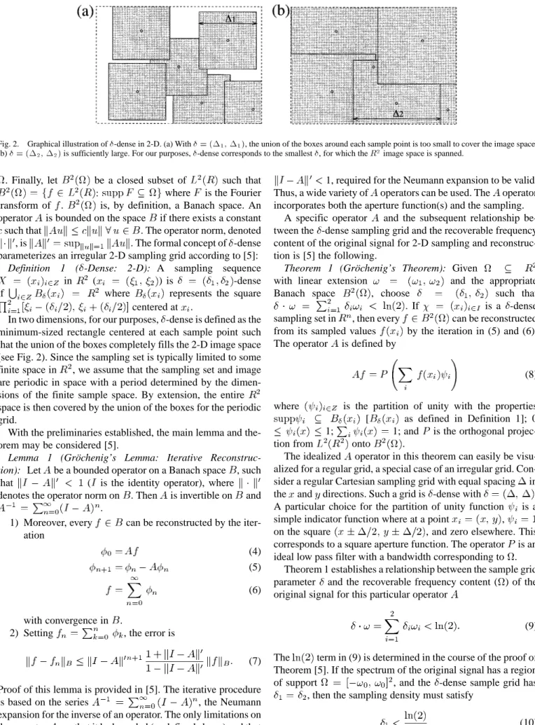
Fig. 2. Graphical illustration of-dense in 2-D. (a) With = (1 ; 1 ), the union of the boxes around each sample point is too small to cover the image space. (b) = (1 ; 1 ) is sufficiently large. For our purposes, -dense corresponds to the smallest , for which the R image space is spanned.
. Finally, let be a closed subset of such that
where is the Fourier transform of . is, by definition, a Banach space. An operator is bounded on the space if there exists a constant
such that . The operator norm, denoted
, is . The formal concept of -dense
parameterizes an irregular 2-D sampling grid according to [5]:
Definition 1 ( -Dense: 2-D): A sampling sequence
in ( ) is -dense
if where represents the square
centered at .
In two dimensions, for our purposes, -dense is defined as the minimum-sized rectangle centered at each sample point such that the union of the boxes completely fills the 2-D image space (see Fig. 2). Since the sampling set is typically limited to some finite space in , we assume that the sampling set and image are periodic in space with a period determined by the dimen-sions of the finite sample space. By extension, the entire space is then covered by the union of the boxes for the periodic grid.
With the preliminaries established, the main lemma and the-orem may be considered [5].
Lemma 1 (Gröchenig’s Lemma: Iterative Reconstruc-tion): Let be a bounded operator on a Banach space , such
that ( is the identity operator), where
denotes the operator norm on . Then is invertible on and .
1) Moreover, every can be reconstructed by the iter-ation
(4) (5) (6)
with convergence in .
2) Setting , the error is
(7) Proof of this lemma is provided in [5]. The iterative procedure
is based on the series , the Neumann
expansion for the inverse of an operator. The only limitations on the operator are that it be bounded (as defined above) and that
1, required for the Neumann expansion to be valid. Thus, a wide variety of operators can be used. The operator incorporates both the aperture function(s) and the sampling.
A specific operator and the subsequent relationship be-tween the -dense sampling grid and the recoverable frequency content of the original signal for 2-D sampling and reconstruc-tion is [5] the following.
Theorem 1 (Gröchenig’s Theorem): Given
with linear extension and the appropriate
Banach space , choose such that
. If is a -dense
sampling set in , then every can be reconstructed from its sampled values by the iteration in (5) and (6). The operator is defined by
(8)
where is the partition of unity with the properties [ as defined in Definition 1]; 0
1; 1; and is the orthogonal
projec-tion from onto .
The idealized operator in this theorem can easily be visu-alized for a regular grid, a special case of an irregular grid. Con-sider a regular Cartesian sampling grid with equal spacing in
the and directions. Such a grid is -dense with .
A particular choice for the partition of unity function is a simple indicator function where at a point ,
on the square , and zero elsewhere. This
corresponds to a square aperture function. The operator is an ideal low pass filter with a bandwidth corresponding to .
Theorem 1 establishes a relationship between the sample grid parameter and the recoverable frequency content ( ) of the original signal for this particular operator
(9)
The term in (9) is determined in the course of the proof of Theorem [5]. If the spectrum of the original signal has a region
of support , and the -dense sample grid has
, then the sampling density must satisfy
This requires the minimum sampling density to be higher than the Nyquist sampling density for a given , or
1.44 times the Nyquist rate for uniformly spaced samples. This “oversampling” is required to ensure reconstruction from the irregular grid. While the sample rate requirements are higher than the Nyquist rate for a uniform grid, this theorem establishes that a function can be completely reconstructed from irregular samples using this particular . The lemma suggests that a va-riety of operators can be used. Thus, for irregular sampling Gröchenig’s lemma and theorem are equivalent to the Nyquist theorem for uniform sampling.
III. RECONSTRUCTIONALGORITHMS
The previous section establishes the validity of signal recon-struction from irregular samples. As long as the signal sam-pling is adequately dense within the Banach space supporting the signal, the original signal can be completely recovered. To apply these formal results in practice, we relate the frequency response of the aperture function to the Banach space and show that Gröchenig’s algorithm is equivalent to block additive alge-braic reconstruction technique (AART) with a modified aperture function. In this section, the relationship of AART to the mul-tiplicative algebraic reconstruction technique (MART) is also explored.
A. Bandlimited Banach Space
As previously noted, the observations can be viewed as ideal samples of an aperture filtered image where the aperture filtered image is the true image convolved with an aperture function. In general, each observation can use a different aperture function so multiple aperture filtered images may need to be considered. For a given aperture function, nulls in the frequency response of the aperture function introduce corresponding nulls in the aperture filtered image. With a single aperture function, image frequencies in the aperture function spectral nulls are lost and cannot be recovered via reconstruction. However, with multiple aperture functions, a net effective aperture function can be de-fined from the appropriately averaged individual measurement aperture functions. Nulls in the effective aperture function cor-respond to the intersection of the nulls of individual aperture functions. So long as the sampling density requirements are met for the remaining frequencies, only frequencies corresponding to the nulls in the net effective aperture function are lost. All other frequencies can be recovered by the reconstruction, sub-ject to the sampling considerations.
While the original image may include information in the nulls of the effective aperture function, for the purposes of analysis, we can redefine the spectral region of support of the original function to exclude the effective aperture function nulls. Within the reduced image space, and subject to adequate sampling, the image can be perfectly reconstructed based on Gröchenig’s Lemma. Image frequencies above those supported by the sam-pling density (i.e., greater than ) cannot be reconstructed and are aliased. The low pass filtering included in the operator fil-ters out such frequencies and for the purposes of analysis, the signal is redefined to exclude frequencies outside of the region of support of the sampling.
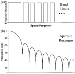
Fig. 3. (a) Bandlimiting scheme that delimits the nulls in the aperture response in (b). The subbands, which can be truncated or continue indefinitely, define a Banach space. (b) Frequency response of a particular aperture function.
Because Lemma 1 requires the operator to be invertible on a Banach space, a Banach space of appropriately bandlimited functions must be established. A simple case is the space of ideal low pass filtered images where the spectrum of the image is lim-ited to . More generally, the spectral content can be lim-ited by the nulls in the effective aperture function. For example, Fig. 3 illustrates a set of truncated band limits imposed around the nulls in the frequency response of a particular effective aper-ture function. It can be shown that such a subband limited space is a Banach space [10]. For adequately sampled data, the image can be completely reconstructed over this space according to Gröchenig’s Lemma, regardless of the aperture function, and we conclude that, in effect, the aperture function’s role is to de-limit the Banach space.
B. Equivalence of AART and Gröchenig’s Algorithm
ART algorithms have been extensively studied in the litera-ture and have been used in reconstruction problems (e.g., [6], [7], [14]). In this section, we compare AART and Gröchenig’s algorithm and show that with an appropriate implementation of AART, they are functionally equivalent in reconstructing images from sampled observations. AART is thus a practical method for image reconstruction from irregular samples.
Gröchenig’s iterative algorithm given in Lemma 1 can be written in the form [5]
(11) where
operator meeting the requirements of Lemma 1; image to be recovered;
estimate of at the th iteration.
Gröchenig’s lemma is valid for a variety of operators with gen-eral conditions and can thus be applied to either continuous or sampled images. In practical application, can generally be assumed to be piecewise continuous on a fine scale. This is consistent with the requirement of a bandlimited (i.e., lowpass)
original image. The image can then be treated as a finely sam-pled or discrete image at this finer scale. We note that this finer sampling is quite different than the measurement sampling grid. It is primarily for computational convenience wherein the image is assumed to consist of discrete uniformly sized pixels much smaller than the measurement sampling. Each noise-free mea-surement or observation covers a number of these small pixels [compare (2)]
(12)
where
elements of the vector of row-scanned image pixels from ;
effective aperture response function for the th mea-surement on the th pixel;
number of pixels in . Block AART can be written as [14]
(13)
where is the th iterative estimate of , and is the back projection
(14)
corresponding to the th measurement at the th iteration with total measurements. In effect, all measurements that “touch” a pixel are summed and normalized to create the per-pixel update.
In (13), the normalized sum term on the right-hand side is a function of the measurement vector and the back projection vector computed from the th iterative estimate. The vector of measurements represents the sampled convolution of the true image with the aperture function. This can be expressed as
a matrix multiplication , where (with elements )
is the sampled aperture function for each measurement. Noting that , (13) can be written as
(15) (16) where the ’s are row-scanned image vectors, and is the
row-normalized transpose of with elements that
perform the summation and normalization in (13). Thus, (13) can be expressed as
(17)
where . Thus, Gröchenig’s algorithm and AART
have the same functional form.
We now wish to show that block AART is equivalent to Gröchenig’s algorithm. The normalized aperture functions in the rows of correspond to the terms in (8). The aperture
function used in the reconstruction must have support on the Banach space defined by both the observation aperture function (which is the case by our definition of the Banach space) and the -dense sampling. To ensure the latter, a low pass filter with a cutoff frequency consistent with the -dense sampling is applied to the aperture functions in the rows of . If this is not done, artifact noise will be introduced in the reconstruction. Hereafter, the aperture function matrices and are assumed to include this low pass filtering. This is the aperture function modification noted earlier. A generalized operator is implicitly included in by this filtering and the use of the fine sampling grid.
We must now show that meets the requirements of Gröchenig’s Lemma. This requires showing that is bounded and invertible on the subband limited Banach space. The fre-quency nulls in the effective aperture response lead to complete loss of information at some frequencies. However, if as dis-cussed earlier, is defined so that it has no frequency content at the nulls and no information is lost, though there may be attenu-ation due to the frequency response of the aperture function. We note that while includes both the observation sampling and aperture function characteristics, in the following discussion, we assume that the sample spacing is adequate for signal recovery and deal strictly with aperture function effects on invertability. How the sample spacing affects the signal recoverability is fur-ther discussed in Section III-C.
The domain of , consists of all functions with
a subband limited frequency response. maps into a range
space . While may null out certain
frequen-cies of an arbitrary input, the domain consists exclu-sively of functions without these frequencies. Therefore, no in-formation is lost for the new problem definition. So for ,
is the projection of onto the columns of , and while may have attenuated frequency components, all the original fre-quency components of are present in . The row normalized transpose of , , is generated by multiplying each row by the sum of the row elements and since elementary row operations
do not affect the rank of the matrix, . Left
multiplication of by , , is also within
the original Banach space. Thus, is a bounded operator on the subband limited Banach space, meeting the first requirement of Lemma 1.
Since the low pass filter has no effect on frequencies within the Banach space, it does not affect invertability of . If is full rank, then is full rank, and the operator is invert-ible on the Banach space. However, it is not necessary that be full rank for the signal to be recoverable. Since by definition no information is lost in the process of applying to an ap-propriately subband limited input function, an appropriate gain function can be defined to compensate for any attenuation. This gain function is the inverse of the attenuation imposed by and thus, is invertible on the subband limited Banach space, meeting the final requirement of Lemma 1.
We therefore conclude that the block AART reconstruction in (17) (with the modified aperture function per the earlier dis-cussion) is equivalent to Gröchenig’s algorithm in (11). Thus, AART represents a valid algorithm for the complete recovery of the original image for an appropriate choice of based
on the aperture function nulls and the sampling density. This result is valid both for irregularly and regularly sampled obser-vations.
A complete reconstruction is only possible if the assump-tion is made that the original funcassump-tion is contained in the space spanned by the operator inverse . However, to avoid having to solve for and explicitly compute within this space, regularization techniques can be used to compute a unique so-lution on the full space. The AART algorithm automatically in-cludes regularization and produces the least squares minimum norm solution. In principle, we can use any of a number of reg-ularization schemes to generate an estimate of the signal for a case where the original function is outside the space spanned by
. This is addressed further in the next section.
C. Signal Recoverability from -Dense Sample Spacing
Given a set of irregular samples that are -dense, the natural question is: what frequency content can be recovered using this grid and an algorithm such as (11) or (13)? While Gröchenig assumed a particular operator in Theorem 1, other opera-tors can be used including the general described. Because the sampling and aperture may vary, generating a prediction of frequency recoverability for a general can be difficult.
However, an upper bound to the frequency recovery is based on the equivalent Nyquist sampling rate. For an arbitrary operator, the recoverable frequency range using an irregular
-dense sampling grid is less than the frequency range re-coverable by a regular -spaced grid as determined by the Nyquist criterion or . A practical limit is the bound
determined in Theorem 1, .
D. Relationship of Additive ART to Multiplicative ART
With the equivalence of block AART and Gröchenig’s algorithm established, we consider the relationship of AART and a close relative, MART. The difference between AART and MART is the regularization implicit in the algorithms. AART is equivalent to a least squares estimate in the limit of infinite iterations [6] based on the minimization problem
Minimize
Subject to (18)
MART with damping is a maximum entropy estimate in the limit of infinite iterations [6], [7] based on the maximization problem
Maximize Subject to
(19)
In effect, AART makes no a priori assumptions about the data and fits the estimate strictly on the measurements available by minimizing the error of the back projection of the measurement onto the space in the mean-squared error (MSE) sense sub-ject to . Thus, the reconstruction is strictly contained within the subband limited Banach space spanned by the mea-surements.
On the other hand, MART effectively assumes a maximum entropy model for the data. In the frequency domain, the recon-struction is not strictly restricted to the bandlimited frequency domain spanned by the measurement space. Additional fre-quency content in the null space may be added by the algorithm to create a sharper image [8]. However, the constraint
remains, and the reconstruction is based on a projection of measurements onto the space, just as in AART.
The choice of one method over another is a debatable issue. We can, in principle, select any regularization to use in the re-construction if the regularization fits with a priori knowledge. As discussed in [6], this decision may be based on the nature of the sampling mechanism (reflection, absorption or emission), and the nature of the solution the algorithm produces for under-determined systems. The choice is dependent on which regular-ization provides the best results for the given application. Least squares estimates (LSEs) produce a maximally smooth estimate where edges tend to be softened and blurred. A maximum en-tropy estimate produces a generally “sharper” image than least squares, at least for images with high contrast [8].
AART and MART enjoy a fundamental relationship based on the common constraint . Since both forms of ART have the same constraint equation, the resulting solutions are of the general form
(20) where is an element of the row space of , or equivalently, the range space of the transpose of , , denoted , and is an element of the null space of , denoted . Any solution derived from either additive or multiplicative ART contains a component . However, the solution derived by using AART results in 0, while the solution from MART gen-erally will have a nonzero component [9]. Since the con-straint is the same for both algorithms, the solutions for both AART and MART are the same in the range space of in the limit of infinite iterations. The only difference between the AART and MART solutions is the component from the null space of , i.e., the AART and MART solutions are the same except in the nulls of the aperture function. If the aperture function does not have nulls, the solutions are identical in the noise-free case. We conclude that both AART and MART are viable reconstruction techniques, with the understanding that in the null spaces, AART and MART may produce slightly dif-ferent results based on the difdif-ferent regularizations.
IV. THEEFFECTS OFMEASUREMENTNOISE
The previous section has shown that AART can completely recover an arbitrary bandlimited function for the noiseless case if the sampling is sufficiently dense. Given adequate sampling, the reconstruction is essentially independent of the aperture function. No matter how low the sidelobes of the aperture data are, the original signal (less the nulls) can be recovered in the limit, at least for noise-free measurements. We now consider two additional issues for reconstruction with iterative algo-rithms. The first is a finite number of iterations, and the second is noise. The former is a practical limitation since no iterative process can proceed indefinitely. Therefore, while a particular
Fig. 4. (Top) Signal and aperture used in the single-aperture simulation. The signal is a narrow sinc function. Dots show the sample values and the irregular locations in the simulation. The arbitrary horizontal scale has been expanded relative to later figures for clarity. (Bottom) Schematic illustration (vertical scale is compressed for clarity) of the spectra of the signal and aperture functions. The signal spectrum is a rect, while the aperture function spectra is asinc .
algorithm converges to a particular solution in the limit, the limit may not be reached when the iteration is terminated. The result is an approximation to the optimal reconstruction, but may not be a complete reconstruction [6]. Truncation of the iterations is ultimately another form of regularization [9].
While Gröchenig’s Lemma shows that complete reconstruc-tion of an irregularly sampled signal can be made, it does not consider the effects of noise. Experimental results show that even highly attenuated frequency components are effectively re-covered with finite iterations for noiseless observations. How-ever, the addition of noise changes the problem because noise is amplified along with the desired signal during the reconstruc-tion. In effect, the reconstruction process can be thought of as a high pass filter that removes the attenuation caused by the aper-ture function, except in the nulls in the aperaper-ture function. The high-pass nature of the reconstruction filter increases the noise power. In Wiener filtering, the reconstruction filter response is modified so that when a specified noise-to-signal ratio threshold is exceeded, the response is set to zero to minimize noise ampli-fication [9]. A similar approach can also be adapted with the techniques discussed in this paper by suitably modifying the filtered aperture function used in the reconstruction. Although steps can be taken to minimize noise, it will, to one degree or another, limit the number of iterations that can be executed be-fore noise overtakes the reconstruction.
A. Algorithm Performance Comparison
Lacking a suitable theoretical analysis of the effects of noise, a Monte Carlo approach is employed to examine the behavior of the signal and noise power in the reconstruction. In the fol-lowing discussion, a simple simulation is used to illustrate the image reconstruction and resolution enhancement of the
algo-Fig. 5. (Bottom) Conceptual illustration of the aperture function and (Top) Reconstruction filter responses.
rithms and compare their performance in the presence of noise. For simplicity of illustration, a one-dimensional (1-D) signal with a bandlimited spectrum is defined with densely sampled measurements synthesized with a fixed aperture function whose frequency response attenuates the high frequency components of the signal spectrum (see Fig. 4). In this simple illustration, the signal is a narrow sinc function, while the aperture function is a wide rect or box-car function. The test signal is densely sampled with an irregular sampling grid. A rectangular aperture function is used in this study so that the first sidelobe of the aperture is within the spectrum of the test signal, as illustrated in Fig. 4, al-lowing the reconstruction of the attenuated frequencies within the sidelobe to be easily evaluated. While the aperture function used here is a constant (rect) window function, similar results are obtained with other window-based aperture functions. Also, though this simulation illustrates recovery of only a single side-lobe, recovery of higher order sidelobes can be accomplished. For each algorithm, both noisy and noise-free cases are consid-ered. For the noisy cases, Monte Carlo white noise is added.
For this example, the spectrum of the ideal reconstruction is the original frequency domain rect, punctuated by the aperture nulls (see Fig. 5). In effect, this filter is applied to the noise component of the measurements in the reconstruction. As illus-trated in Fig. 5, as the wave number increases, the reconstruction gain increases, resulting in a corresponding increase in the noise power. Thus, increasing the bandwidth of the reconstruction re-sults in greater noise power at high frequencies, lowering the SNR. If the initial SNR is adequate, this is not a problem, but at some point, the noise power may exceed an acceptable level.
While a variety of other related reconstruction algorithms exist (e.g., [11]–[13]), we here consider only one additional algorithm, the scatterometer image reconstruction (SIR) algo-rithm. The algorithm is a derivative of MART developed for multivariate scatterometer image reconstruction with noisy measurements [1]. A single-variate form has been used for radiometer resolution enhancement [2] and is the form consid-ered in this paper. Although similar in performance to MART, SIR is more robust in the presence of noise, particularly at low SNRs, and is thus a useful alternative to AART and MART.
Fig. 6. Comparison of AART, MART, and SIR outputs after 30, 100, and 1000 iterations for noiseless measurements. The ideal output is a sinc function.
B. Noisy Versus Noise-Free Observations
To evaluate the algorithm performance, both noise-free and noisy measurements are used. Further, since the algorithms can only be run a finite number of iterations, the performance as a function of iterations is also considered.
Fig. 6 compares the output of the three algorithms at 30, 100, and 1000 iterations without noise. There are two significant ob-servations from these results: First, the algorithms are able to provide good reconstruction of the original signal. Second, there is an apparent lag (as a function of the number of iterations) of the SIR and MART results compared to the AART output. This lag is a result of the damped multiplicative update factor used in the MART and SIR algorithms.
Fig. 7 illustrates the spectra of the output for 1000 iterations of all three algorithms (compare the sidelobe levels in this figure to those in Fig. 4). After processing, the full test signal band-width (excluding the nulls) is essentially recovered. All three al-gorithms successfully reconstruct the original signal within the limits imposed by the aperture function nulls as predicted by the theoretical development.
To evaluate the performance with noise added, Fig. 8 presents the spectra of the output from AART, MART, and SIR at 30 and 1000 iterations for both noiseless and noisy cases. We note that the performance of AART in the presence of noise is sig-nificantly degraded. This observation originally motivated the development of SIR [1]. For both MART and SIR, the multi-plicative update factors are damped so that large update factors do not overly magnify the noise at any one iteration. SIR incor-porates a nonlinear damping, which can further reduce the noise at the expense of slower reconstruction.
C. Reconstruction Error
We now consider the relationship between the number of it-erations and the quality of the reconstructed image. In general, iterative reconstruction suffers from two forms of error: recon-struction error and noise amplification. The reconrecon-struction error is the difference between the iterative image estimate and the noiseless true image. Noise amplification results from the in-verse filtering of the noise, as previously noted [6], [9].
A graph of the RMS errors (RMSEs) versus iteration number for the simulation is presented in Fig. 9. The graph shows the
Fig. 7. Frequency domain comparison of the outputs of AART, MART, and SIR after 1000 iterations in the noiseless case. Vertical scale is linear. The ideal spectrum is a rect. After additional iterations, MART and SIR results become essentially identical to the AART results.
Fig. 8. Spectra of the output of AART, MART, and SIR at different iterations for noiseless and noisy measurements. Vertical scale is linear.
Fig. 9. Comparison of the RMS errors for AART, MART, and SIR versus iteration number. Each curve represents a separate application of the algorithm to compute the RMS signal error (Es), the noise-only RMS error (En), and the signal plus noise RMS error (E).
noise amplification error (En), the reconstruction error (Es), and the total error (E) for the signal plus noise for ARRT, MART, and SIR. The errors are computed as the RMS of the pixel-by-pixel difference between the true and the reconstructed images at each iteration. In the simulation, separate reconstructions are run for case to evaluate the RMS error.
Considering Fig. 9, we note that at any given iteration, the reconstruction error is smaller and the noise amplification is greater for ARRT than for MART and SIR. The total error for AART reaches a minimum after just a few iterations but grows rapidly as the iteration continues. SIR and MART reach minima in the total error more slowly but eventually achieve lower levels of total error.
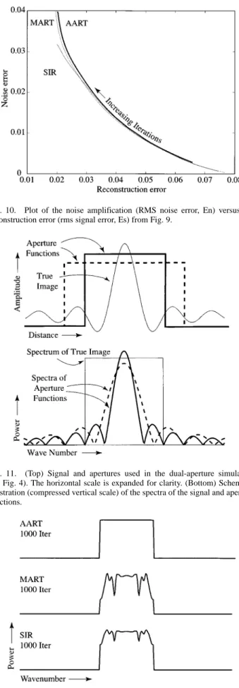
The difference in noise amplification for the various algo-rithms is further illustrated in Fig. 10. This graph shows a plot of the noise amplification versus the reconstruction error. While the overall performance of the algorithms are similar, at lower reconstruction errors MART and SIR have lower noise ampli-fication than AART. At the lowest reconstruction errors, SIR has the smallest noise. In all cases, there is a tradeoff between reconstruction error and noise amplification controlled by the number of iterations. We note that the differences become more apparent at lower SNRs.
It should be noted that while the RMSE is an indicator of the accuracy of the reconstruction, the size and location of the error changes over the course of the iteration depending on the regu-larization [9]. Also, the quality of the resulting imagery may not always be a direct function of total error [8]. The image quality for SIR at a given reconstruction error level is subjec-tively somewhat better than corresponding MART or AART products when used with scatterometer data [1].
D. Multiple Aperture Functions
In the simulation example presented previously, irregular sampling with a fixed aperture function was employed. The single aperture function introduces a null in the estimated signal spectrum. However, when the aperture functions exhibit variability between measurements, this null can be eliminated if the nulls of the various aperture functions do not intersect and the sampling is adequately dense. To illustrate this, the noise-free simulation previously described is modified so that each measurement randomly uses either the original aperture function or a wider (lower resolution) aperture function, as illustrated in Fig. 11. Simulation reveals that the spectra of the estimated signal does not exhibit data loss due to an aperture null. The signal is completely reconstructed in the noise-free case, as illustrated in Fig. 12. Noisy simulations yield con-clusions regarding the relative performance of the algorithms consistent with the previous section.
This result suggests a useful strategy in the design and ap-plication of remote sensing instruments to optimize their reso-lution enhancement capability during postprocessing. While a minimum size aperture function yields the finest effective res-olution, it is often possible to alter the “shape” of the effective aperture. When adequately dense sampling is available, mea-surements from elongated aperture functions with variable ori-entations can prevent the occurrence of spectral nulls in the re-constructed images. Including sampling and aperture function
Fig. 10. Plot of the noise amplification (RMS noise error, En) versus the reconstruction error (rms signal error, Es) from Fig. 9.
Fig. 11. (Top) Signal and apertures used in the dual-aperture simulation (cf. Fig. 4). The horizontal scale is expanded for clarity. (Bottom) Schematic illustration (compressed vertical scale) of the spectra of the signal and aperture functions.
Fig. 12. Frequency domain output of AART, MART, and SIR after 1000 iterations in the noiseless dual aperture function case. After additional iterations, the MART and SIR outputs match the AART output. The ideal spectrum is a rect. Vertical scale is linear. Note the absence of nulls in the signal spectra (cf. Fig. 7) when multiple aperture functions are used.
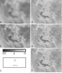
Fig. 13. Images generated from actual ERS-2 and SeaWinds scatterometer data. (a) Gridded ERS-2 image, (b) SIR-processed ERS-2 image, and (c) representative 3-dB instrument footprints to scale with images. The circle corresponds to the ERS-2 50-km diameter footprint, while the other shapes are representative SeaWinds slice footprints which vary in size and orientation. (d) Gridded SeaWinds image, (e) SIR-processed SeaWinds image, and (f) SIR with modified median filter-processed SeaWinds image. Images show the normalized radar cross section adjusted to a 40 incidence angle “A in dB.”
considerations in the design of the sensor system can result in improved resolution.
We note that increased sampling density can be achieved by combining multiple passes over the study area [1], [11]. Assuming that the study area does not change between passes, combining multiple overpasses can provide a dense sampling of the image area. Of course, accurate position information for the individual samples is required. This approach can be used to provide improved resolution images from sensors with single-pass sampling otherwise inadequate for applying the reconstruction algorithm to enhance the effective resolution. Combining multiple passes has been successfully employed with scatterometer data [1], [15]–[17] and is used in the next section. The ultimate limits to such an application are the sampling density, nulls introduced by the aperture function(s), the acceptable noise level, and the temporal stability of the study area [1].
V. ACTUALDATA
The analysis presented thus far has been based on 1–D simu-lations. We now illustrate the 2–D application of the reconstruc-tion theory with actual data, considering two sensors, one with a fixed aperture and one with a variable aperture sensor. While the technique can be used for many types of sensors, data from two microwave scatterometer systems are used: the C-band Eu-ropean Remote Sensing Satellite (ERS-2) [18] and the Ku-band SeaWinds on QuikScat [19]. Originally designed for wind mea-surement over the ocean, these sensors measure the normalized radar cross section of the ocean’s surface from which the wind is inferred. Scatterometer data can also be used for land and ice studies, e.g., [15]–[17]. In this analysis, the study area is a 868
Fig. 14. Center locations of ERS-2 measurements used in Fig. 13. SeaWinds measurements have a similar but much more dense irregular sampling pattern. A plot of the SeaWinds measurement locations is completely black and thus is not shown.
km 668 km region of northern Mexico and southern Texas centered at 102.5 E, 27 N.
The ERS-2 scatterometer measurements have a Hamming window aperture function with a 3-dB width of 50 km [see Fig. 13(c)] [20]. While the ERS-2 scatterometer data is reported on a 25 km satellite track-based grid, combining multiple passes (and assuming the surface is constant) results in a much finer surface sampling. A 30-day (JD 280-310, 1996) imaging pe-riod is used for ERS-2 data, resulting in a -dense sampling of approximately 10 km (see Fig. 14). The SeaWinds “slice” measurements have variable aperture functions with an effective size of approximately 7 km 30 km [see Fig. 13(c)] [19]. The eight days (JD 230-237, 2000) of SeaWinds data used produce a -dense sampling better than 1 km. In both cases, the scat-terometer measurements are normalized to an incidence angle of 40 . The noisy ERS-2 measurements have a normalized stan-dard deviation of approximately 5%. The SeaWinds slice mea-surements are generally much noisier than the ERS-2 measure-ments.
Both gridded and SIR reconstructed images created from the scatterometer measurements are shown in Fig. 13. The gridded images are produced using the “drop-in-the-bucket” technique with pixel sizes of 22 km and 11 km for ERS-2 and SeaWinds, respectively. Each pixel value is defined as the average of all the measurements that have a center location falling within the grid element. Since the effective resolution of gridded images is limited by the resolution of the measurements, the grid size is set to about half the measurement resolution. The gridded images are expanded to match the size of the reconstructed images. For the SIR reconstructed measurements, the reconstruction is done on a 2.225 km grid using 200 iterations. In Fig. 13(f), a modified median filter [1] is incorporated in the SIR processing to reduce the effects of the noise enhancement at the expense of some loss of resolution.
Comparison of the gridded and reconstructed images in Fig. 13 clearly reveals the improvement of the detail in the re-constructed images. The rere-constructed SeaWinds image shows the noise enhancement effect of the reconstruction, though this is ameliorated when the modified median filter is used. Noise enhancement in the ERS-2 reconstructed image is less obvious due to the lower noise level of the ERS-2 measurements.
Although the two sensors operate at different frequencies, similar features are visible in the image sets, albeit at different effective resolutions. The dark feature in the center of the study area is a valley containing the lake Laguna de Mayran. To the north of the valley are the Sierra de Los Alamitos mountains,
part of the Sierra Madre Oriental range that makes up the near-vertical light band. Due to the corner reflector effect, urban areas show up as light dots in the images. For example, the white area in the upper right corner is San Antonio, TX. This feature is clearly visible in the SeaWinds images and in the reconstructed ERS-2 image but is difficult to distinguish in the gridded ERS-2 image. Similarly, Monterrey, Mexico is to the lower-right of image center. Though the resolution of the reconstructed images is very coarse when compared to synthetic aperture radar (SAR) images, scatterometer data is available over a multidecadal pe-riod and has frequent global coverage.
VI. SUMMARY ANDCONCLUSIONS
This paper has discussed the theory of image reconstruction from irregularly sampled data. The relationship between the aperture function, the measurement sampling, and the recon-struction has been examined. Gröchenig’s lemma was presented to demonstrate that a signal can be completely recovered from irregular samples. When the sampling is sufficiently dense, the attenuation introduced by the aperture function can be com-pensated for, resulting in a complete reconstruction exclusive of the spectral nulls in the effective aperture function. Addi-tive ART with suitable modification was shown to be equiva-lent to Gröchenig’s algorithm. MART and AART solutions were shown to be identical in the Banach space defined by the effec-tive aperture function’s spectral nulls. Simulation was used to demonstrate the reconstructive abilities of AART, MART, and SIR for noise-free and noisy cases.
The ART and SIR algorithms can be termed resolution en-hancement algorithms because of their ability to fully recon-struct attenuated signal components. SIR is more robust than MART and AART in the presence of noise. Finally, when the aperture area is fixed but a sufficiently high sampling density is possible, elongated aperture functions with a diversity of over-lapping orientations can yield the best possible resolution en-hancement in postprocessing algorithms.
We conclude that for suitably designed or modified sampling, image reconstruction and resolution enhancement algorithms such as AART, MART, and SIR can be an effective way to increase the effective resolution of remotely sensed imagery. Since the algorithms are typically applied in postprocessing, they can be an inexpensive method for achieving higher reso-lution data products. We further note that improved reconstruc-tion/resolution enhancement performance can be achieved if the sampling and aperture function considerations for optimum res-olution are included as part of the design process of the sensor system.
APPENDIX
ALGORITHMDESCRIPTIONS
Because of the varying notation used in the primary ref-erences, a brief summary of the block AART, block MART, and radiometer SIR algorithms is provided in a consistent notation. Finely sampled images are represented as vectors of
row-scanned pixels: in an image with pixels,
the pixel maps to element of the image
vector. The noise-free observations of the true image are
(21)
where is the aperture response function for the th measure-ment on the th pixel. The matrix with elements is formed by applying the appropriate low pass filter (with bandwidth defined by the -dense sampling) to each row of the matrix such that the rows of are the low pass filtered rows of . is the row-normalized transpose of . At the th iteration, the forward projection is
(22) The iterative AART, MART, and SIR algorithms require an initial image , usually a constant. MART and SIR require that all the measurements and image pixels (at all iterations) have the same algebraic sign.
The block AART algorithm is
(23) while block MART is
(24)
where is the damping factor, typically 1/2. SIR is
(25)
where
(26)
where . For the linearized form of SIR,
is used rather than (26).
ACKNOWLEDGMENT
SeaWinds data were obtained from the PODAAC at the Jet Propulsion Laboratory, Pasadena, CA.
REFERENCES
[1] D. Long, P. Hardin, and P. Whiting, “Resolution enhancement of space-borne scatterometer data,” IEEE Trans. Geosci. Remote Sensing, vol. 31, pp. 700–715, May 1993.
[2] D. Long and D. Daum, “Spatial resolution enhancement of SSM/I data,”
IEEE Trans. Geosci. Remote Sensing, vol. 36, pp. 407–417, Mar. 1998.
[3] A. V. Oppenheim and A. S. Willsky, Signals and Systems. Englewood Cliffs, NJ: Prentice Hall, 1983.
[4] H. Freichtinger and K. Gröchenig, “Iterative reconstruction of multi-variate band-limited function from irregular sampling values,” SIAM J.
Math. Anal., vol. 23, no. 1, pp. 244–261, 1992.
[5] K. Gröchenig, “Reconstruction algorithms in irregular sampling,” Math.
Comput., vol. 59, no. 199, pp. 181–194, 1992.
[6] Y. Censor, “Finite series-expansion reconstruction methods,” Proc.
[7] T. Elfving, “On some methods for entropy maximization and matrix scaling,” Lin. Algebra Applicat., no. 34, pp. 321–339, 1980.
[8] A. K. Jain, Fundamentals of Digital Image Processing. Englewood Cliffs, NJ: Prentice-Hall, 1989.
[9] R. L. Lagendijk and J. Biemond, Iterative Identification and Restoration
of Images. Boston, MA: Kluwer, 1991.
[10] D. E. Early, “A study of the scatterometer image reconstruction algorithm and its application to polar ice studies,” Ph.D. dissertation, Brigham Young Univ., Provo, UT, May 1998.
[11] B. G. Baldwin, W. J. Emery, and P. B. Cheeseman, “Higher resolution earth surface features from repeat moderate resolution satellite imagery,”
IEEE Trans. Geosci. Remote Sensing, vol. 36, pp. 244–255, Jan. 1998.
[12] W. D. Robinson, C. Kummerow, and W. S. Olson, “A technique for en-hancing and matching the resolution of microwave measurements from the SSM/I instrument,” IEEE Trans. Geosci. Remote Sensing, vol. 30, no. 3, pp. 419–429, May 1992.
[13] M. A. Goodberlet, “Improved image reconstruction techniques for syn-thetic apertur radiometers,” IEEE Trans. Geosci. Remote Sensing, vol. 38, pp. 1362–1366, May 2000.
[14] P. Gilbert, “Iterative methods for the three-dimensional reconstruction of an object from projections,” J. Theoret. Biol., vol. 36, pp. 105–117, 1972.
[15] D. G. Long and M. R. Drinkwater, “Greenland observed at high res-olution by the Seasat-A scatterometer,” J. Glaciol., vol. 32, no. 2, pp. 213–230, 1994.
[16] D. G. Long and P. Hardin, “Vegetation studies of the Amazon Basin using enhanced resolution SEASAT scatterometer data,” IEEE Trans.
Geosci. Remote Sensing, vol. 32, pp. 449–460, Mar. 1994.
[17] D. G. Long and M. R. Drinkwater, “Cryosphere applications of NSCAT data,” IEEE Trans. Geosci. Remote Sensing, vol. 37, pp. 1671–1684, May 1999.
[18] E. P. Attema, “The active microwave instrument on-board the ERS-1 satellite,” Proc. IEEE, vol. 79, pp. 791–799, June 1991.
[19] M. W. Spencer, C. Wu, and D. G. Long, “Improved resolution backscatter measurements with the SeaWinds pencil-beam scatterom-eter,” IEEE Trans. Geosci. Remote Sensing, vol. 38, pp. 89–104, Jan. 2000.
[20] J. L. Alvarez-Perez, S. J. Marshall, and K. Gregson, “Resolution im-provement of ERS scatterometer data over land by Wiener filtering,”
Remote Sens. Environ., vol. 71, pp. 261–271, 2000.
David S. Early (M’93) received the B.S. and Ph.D. degrees in electrical
engi-neering from Brigham Young University, Provo, UT, in 1993 and 1999, respec-tively.
His graduate work in the Microwave Earth Remote Sensing Laboratory, Brigham Young University, Provo, UT, focused on algorithm development for resolution enhancement of spaceborne scatterometers, specifically the theory behind the algorithms and the application of resolution-enhanced scatterometer data to southern ocean sea ice. After graduation, he worked in the telecommunications industry developing advanced network modeling techniques and predictive planning methods for next generation data networks.
Dr. Early received a 1993 NASA Global Change Fellowship.
David G. Long (M’79–SM’98) received the Ph.D.
in electrical engineering from the University of Southern California, Los Angeles, in 1989.
From 1983 to 1990, he was with the NASA’s Jet Propulsion Laboratory (JPL), Pasadena, CA, where he developed advanced radar remote sensing systems. While at JPL, he was the Project Engineer on the NASA Scatterometer (NSCAT) Project, which was flown aboard the Japanese Advanced Earth Observing System (ADEOS) from 1996 to 1997. He also managed the SCANSCAT project, the predecessor to SeaWinds. He is currently a Professor in the Electrical and Com-puter Engineering Department, Brigham Young University, Provo, UT, where he teaches upper division and graduate courses in communications, microwave remote sensing, radar, and signal processing. He is the Principle Investigator on several NASA-sponsored interdisciplinary research projects in remote sensing including innovative radar systems, spaceborne scatterometry of the ocean and land, and modeling of atmospheric dynamics. He is a member of the NSCAT and SeaWinds Science Working Teams. He has numerous publications in signal processing and radar scatterometry. His research interests include microwave remote sensing, radar theory, space-based sensing, estimation theory, computer graphics, signal processing, and mesoscale atmospheric dynamics.