Commit-Level vs. File-Level
Vulnerability Prediction
by
Michael Chong
A thesis
presented to the University of Waterloo in fulfillment of the
thesis requirement for the degree of Master of Applied Science
in
Electrical and Computer Engineering
Waterloo, Ontario, Canada, 2016
c
I hereby declare that I am the sole author of this thesis. This is a true copy of the thesis, including any required final revisions, as accepted by my examiners.
Abstract
Helping software development teams find and repair vulnerabilities before they are re-leased and exploited can prevent costs due to loss of data, availability, and reputation. However, while general defect prediction models exist to help developers find bugs, vul-nerability prediction models currently do not achieve high enough prediction performance to be used in industry [43]. Prediction of vulnerabilities in commits and files has been explored by previous work, and while commit-level prediction, at a finer granularity, may offer more useful results, there exists no clear comparison in predictive performance to justify this assumption.
To inform further research in vulnerability prediction, we compare commit and file-level prediction, across 7 projects, using 6 classifiers, for 8 different training dates. We evaluate the performance of each prediction model using ‘online prediction’ for ensuring an evaluation in line with practical usage of the prediction model. We evaluate each model using four different metrics, which we interpret as representing two different practical usage scenarios. We also perform an analysis of the data and techniques for evaluating prediction models. We find that despite achieving a low absolute prediction performance, file-level prediction generally tends to outperform commit-level prediction, but in a few outstanding cases, commit-level performs better.
Acknowledgements
I would like to thank my advisor, Lin Tan, for guidance, advice, and patience with my work on this research. I would like to thank fellow members of the asset team (present and past) who have helped contribute to this research, particularly Thibaud Lutellier, but also Song Wang, Ming Tan, and Nasir Ali, as well as other member who provided helpful advice, feedback, and inspiration. I would also like to thank the VCCFinder team for sharing their results and source code, which facilitated the replication of their results.
Dedication
Table of Contents
List of Tables ix
List of Figures x
1 Introduction 1
1.1 Developing a Practical Technique . . . 3
1.2 Contributions . . . 4
2 Vulnerability Prediction 6 2.1 Generating a Training Set . . . 7
2.2 Training a Prediction Model . . . 7
2.3 Predicting Vulnerabilities . . . 7 2.4 Online Prediction . . . 7 2.5 Labelling instances . . . 8 2.6 Feature extraction . . . 11 2.7 Evaluation Measures . . . 11 3 Study Design 14 3.1 Features . . . 14
3.1.1 Code Churn features . . . 15
3.1.3 Complexity Metrics . . . 15
3.1.4 Keywords . . . 17
3.2 Training and Test Sets . . . 17
3.3 Research Question . . . 20
4 Experimental Setup 21 4.1 Projects under study . . . 21
4.2 Classification algorithms and tuning . . . 22
4.3 Preprocessing steps . . . 23
4.4 Implementation and Runtime . . . 23
5 Findings 26 5.1 Comparison of prediction performance and cost effectiveness . . . 26
5.2 Cases with higher commit-level performance . . . 28
5.3 AUROC vs. AUCEC . . . 29
6 Prediction Data Analysis 34 6.1 Finding vulnerability fixing commits . . . 34
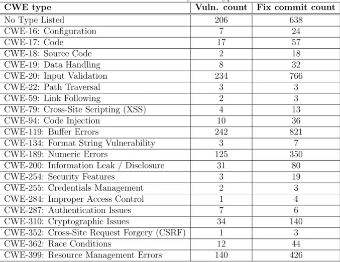
6.2 Types of vulnerabilities found in projects . . . 37
6.3 Vulnerability time to fix . . . 37
6.4 Sample feature distributions . . . 39
7 Threats to Validity 44 8 Related Work 46 8.1 Defect and Vulnerability Prediction . . . 46
8.2 Vulnerabilty Prediction in binaries . . . 46
8.3 File-Level Prediction . . . 47
8.4 Commit-Level Prediction . . . 47
9 Conclusion 49
9.1 Future Work . . . 50
References 52
APPENDICES 61
A Classifier Performances by Project, Level and Metric 62
B ROC and CE curve comparisons for Naive Bayes classifier, Jan 2013 68
C Vulnerability CWE types by project 74
D Vulnerability time to fix histogram by project 78
List of Tables
3.1 List of features extracted. . . 16
4.1 Projects under study. . . 22
4.2 Classifiers under study. . . 22
6.1 Labelling Vulnerable Instances. . . 35
6.2 Vulnerability CWE types . . . 38
C.1 Vulnerability CWE types by project. . . 75
C.2 Vulnerability CWE types by project - continued . . . 76
C.3 Vulnerability CWE types by project - continued (2) . . . 77
E.1 Keyword Features . . . 85
List of Figures
2.1 Labelling vulnerable (‘buggy’) instances. . . 10
3.1 Training and testing sets for file- and commit-level prediction . . . 18
5.1 Naive Bayes performances by project, level, and metric. . . 28
5.2 ROC and CE curves, commit and file level, for PHP, Naive Bayes classifier, and Jan 2013 test date. . . 32
5.3 ROC and CE curves, commit and file level, for FFmpeg, Naive Bayes clas-sifier, and Jan 2013 test date. . . 33
6.1 Vulnerability times to fix in years, showing both density and cumulative density estimation. . . 39
6.2 Paired plots - Commit level . . . 42
6.3 Paired plots - File level . . . 43
A.1 J48 performances by project, level, and metric.. . . 63
A.2 ADTree performances by project, level, and metric. . . 64
A.3 Multilayer Perceptron performances by project, level, and metric. . . 65
A.4 Logistic regression performances by project, level, and metric. . . 66
A.5 Random Forest performances by project, level, and metric. . . 67
B.1 ROC and CE curves, commit and file level, for httpd, Naive Bayes classifier, and Jan 2013 test date. . . 69
B.2 ROC and CE curves, commit and file level, for Kerberos, Naive Bayes clas-sifier, and Jan 2013 test date. . . 70 B.3 ROC and CE curves, commit and file level, for OpenSSL, Naive Bayes
clas-sifier, and Jan 2013 test date. . . 71 B.4 ROC and CE curves, commit and file level, for Wireshark, Naive Bayes
classifier, and Jan 2013 test date. . . 72 B.5 ROC and CE curves, commit and file level, for Xen, Naive Bayes classifier,
and Jan 2013 test date. . . 73 D.1 Vulnerability times to fix in years for Apache httpd, showing both density
and cumulative density estimation. . . 79 D.2 Vulnerability times to fix in years for Kerberos, showing both density and
cumulative density estimation. . . 80 D.3 Vulnerability times to fix in years for OpenSSL, showing both density and
cumulative density estimation. . . 81 D.4 Vulnerability times to fix in years for Wireshark, showing both density and
cumulative density estimation. . . 82 D.5 Vulnerability times to fix in years for Xen, showing both density and
Chapter 1
Introduction
High-profile disclosures of software vulnerabilities continue to make headlines with in-creasing frequency. Software vulnerabilities (permission errors, buffer overflows, or SQL injections, for example) are bugs that a malicious attacker may “exploit to cause loss or harm” [52]. The public disclosure of a vulnerability can take a financial toll on a company’s stock prices [74], and the cost of developing and deploying a patch can be expensive [63]. Additionally, vulnerabilities expose users to attacks that may reveal or disrupt sensitive data or services, and these attacks can also have a significant financial impact—it has been estimated that they cost the global economy more than $400 billion annually[5]. Because of the significant impact and cost of vulnerabilities, research on new tools to help developers identify and repair vulnerabilities is crucial.
Vulnerability prediction techniques, based on related work in defect prediction, have been developed to predict elements of software (files, binaries, changes, or commits) that are likely to contain vulnerabilities. They do so by leveraging ‘features’, or attributes that characterise the elements they are predicting on. Features such as code complexity, developer activity metrics, or source code keyword metrics are used for this purpose. These prediction models can be applied at varying levels of granularity, including binary [79], component [48], file [68], commit [50] and change [31,73]. At each level of granularity, the classification performance and utility (or cost effectiveness) of vulnerability prediction may vary. These variations may be due to differences in element size, semantics and distribution of element attributes (‘features’), and frequency of vulnerable elements.
Vulnerability prediction techniques proposed at different levels of granularity have ob-tained various degrees of success, and some recent studies have been investigating which level of granularity is the most promising to work with [54, 43]. In particular, Morrison
et al. [43] examine vulnerability prediction at binary level and file level. They suggest that vulnerabilities predicted at file level provide information that is more useful to de-velopers than those predicted at binary level, but find that when compared, file-level has worse (i.e., lower) prediction performance results. Posnett et al. [54], examine defect pre-diction in general and compare package-level prediction with file-level prediction. In line with Morrison et al.’s results, they find that prediction at file level provides comparable or worse performance than at package level, measured in terms of traditionally used metrics measuring classification performance. However, they also evaluate classification using‘cost effectiveness’ metrics, and find that file-level prediction is significantly more cost effective than prediction at a higher level of granularity. Based on these results, one might conclude that the finer granularity of file-level prediction is more useful, but harder to do, than the coarser grained package and binary-level prediction.
While thefile-level prediction models discussed above predict which files are vulnerable in a given version of a project, commit-level prediction[50] predicts which commits, made over a project’s history, are vulnerable. File-level prediction models are often trained using past versions of the project, where each file is labelled as “vulnerable” (containing a vulnerability), or “clean” (no vulnerability yet found) [68]. On the other hand, commit-level models are trained using past commits labelled as “vulnerable” (commits introducing a vulnerability), or “clean”.
One might expect based on the studies [43], and [54], discussed above, that commit-level prediction, at a finer granularity, would be more useful for developers, but have worse prediction results. However, a recent study, VCCFinder [50], proposed a method to predict vulnerabilities at commit level that obtained a comparable performance to previous vulnerability prediction at file level [68]. However, they achieve this performance on a different dataset, and using a different machine learning algorithm. A direct comparison between commit- and file-level vulnerability prediction, to the best of our knowledge, has yet to be performed.
As discussed by Morrison et al., while general defect prediction has achieved high enough performance that it is currently being employed in industry by software devel-opment companies like Microsoft, vulnerability prediction has yet to achieve acceptable performance for practical use in industry [43]. For this reason, our work seeks to provide insight to further inform the development of vulnerability prediction towards the develop-ment of practical industry tools. In order to find out which level of granularity it would benefit us most to develop further with improved vulnerability-specific attributes and pre-diction techniques, a direct comparison of the two prepre-diction granularities is required.
Is commit-level vulnerability prediction better than file-level vulnerability prediction? Commits and files have different semantics and attribute sets that may benefit one over the other, and which make direct comparison of the two prediction granularities nontrivial. For example, in mature projects, commits generally contain fewer lines of code than files, while there exist many more commits over the project’s history than there are files in a given version. In addition, while files, packages, and projects (“binary level”), share a hierarchical relationship (e.g., projects, packages contain a set of files), and analogous features can be calculated through aggregation, the same is not true for commits and files. This means that there are some differences in the semantics and distribution of ‘features’, or attributes, used at file level versus those used at commit level. Because of these differences, a set of features that may work well for one granularity level (file or commit) may not map directly to the other. For example, features of the commit message, or the commit time, may contribute to prediction performance for commit-level prediction [31, 50, 73], but these have no direct analogy at file level. On the other hand, cyclomatic complexity may be less meaningful at commit level, as a commit contains additions and deletions to lines in a file, and does not intuitively have a program path.
Our research seeks to develop as fair a comparison as possible, built on the same projects over the same time periods, and using a variety of features and their analogies at both commit and file level, in order to directly compare the two prediction granularities. By doing so, we hope to inform further research in vulnerability prediction by providing insight into which level of granularity performs better, and how each level of granularity is impacted by current techniques used for evaluating prediction performance.
1.1
Developing a Practical Technique
In the end, this research is motivated to facilitate the development of techniques that can be used practically in industry in order to aid software development teams find and fix vulnerabilities before they are released and can be exploited. To that end, we design both our experiment and our evaluation to reflect, as much as possible, the effectiveness of prediction for such practical, real-world use. We choose an experiment design based on the Online Prediction [73] technique, which simulates the practical use of a classifier for real-world prediction on a software project. We argue that Online Prediction is a more rigorous process of evaluation, due to the challenges it poses through the introduction of undiscovered vulnerabilities, as discussed in Section2.4. For our evaluation, we explore a variety of different classifier performance metrics to compare two different usage scenarios, similar to the evaluation performed by [54].
When evaluating prediction models, traditional techniques, such as k-fold cross valida-tion can result in evaluavalida-tions with artificially high accuracy and precision when compared with performance of models used in production [73]. As such,Online Prediction was devel-oped in order to accurately evaluate prediction performance in a real-world setting. When training a prediction model, instances (files or commits) from before a “training date” are collected to be used as a training set. However, if vulnerabilities that have been discovered after the training date are used to label training instances for an evaluation, the resulting performance of the classifier will be at an advantage from this use of “future data” (this also occurs in k-fold cross validation). This means that a production classifier built to detect vulnerabilities in recent project versions or commits may not perform as well as in an evaluation.
Previous work [68, 50, 43] then evaluates the results of the prediction based on criteria derived from the confusion matrix of the classification results, which present the classi-fication errors, False Positives (FPs) and False Negatives (FNs), as well as the correctly classified True Positives (TPs), and True Negatives (TNs) (as described further in Sec-tion2.7). Posnett et al. argue that evaluating defect prediction based on ‘cost effectiveness’ metrics, that is, the number of vulnerabilities discovered versus the number of lines of code inspected to find those vulnerabilities, is a more rigorous and higher standard with which to measure performance. They also argue that it is more accurately represents the practical utility of the classifier. In our evaluation, we propose two usage scenarios represented by different metrics and capturing different possible uses of the classifier. The ‘classification performance’ usage scenario, measured by traditional classification performance metrics F1 score and AUROC (discussed in Section 2.7), evaluates the quality of prediction if all
vulnerable instances as predicted by the classifier are able to be examined. On the other hand, the ‘cost effectiveness’ usage scenario, measured by AUCEC and TPR10k (again discussed in detail in Section2.7), evaluates how many vulnerable instances are discovered by examining instances in order of likelihood, and at a cost equivalent to the instance size. We use these two usage scenarios to describe how the evaluation metrics we use can be interpreted. The comparison of usage scenarios is discussed in more detail in Section 3.3.
1.2
Contributions
In this project, we compare the performance of vulnerability prediction at file level and commit level using an analogous set of features for each level of granularity. Our evaluation uses the online prediction method in order to present results that represent actual practical usage of a classifier. We perform the comparison on 7 projects, for 6 classifiers, and for
8 training dates, and present both ‘classifier performance’ and ‘cost effectiveness’ results. We also present an in-depth analysis of the data used in our evaluation and the process used to extract it, in order to gain insight on the techniques we used, (techniques based on those used in previous work), the data we collected, and its impact on our evaluation of vulnerability prediction performance. We find that for both ‘classifier performance’ and ‘cost effectiveness’, file-level prediction usually outperforms commit-level prediction. We also find that for some projects and classifiers, particularly the PHP project and J48 classifier, median AUROC and AUCEC scores are higher at commit level than file level. Finally, we note that for some ROC and CEC curves, one level of granularity may perform better below certain low thresholds (5% false postive rate for ROC curve or under 20% LOC for CEC curve), while overall the other level of granularity shows a higher prerformance.
This project makes the following contributions:
• A comparison of the effectiveness of commit-level and file-level vulnerability predic-tion using analogous features for each. We perform our comparison on 7 different projects, with vulnerability labelling data collected using an automated technique, using independently tuned project-specific heuristics to match vulnerabilities with fixing commits. We use four different metrics describing two different usage scenar-ios to evaluate the performance of our classifiers
• We find that file-level prediction generally outperforms commit-level under all met-rics. However, we also find that for certain projects, in particular the PHP project, commit-level sometimes outperforms file-level under AUROC and AUCEC metrics. • We produce a dataset including features/attributes of files and commits from the
history of each of the 7 projects, labelled with vulnerability data from the National Vulnerability Database using variable training dates. It can be easily extended to in-clude other projects, features/attributes, and training dates. It can also be extended to compare commit- and file-level general defect prediction on the same projects. The remainder of the work is organized as follows: Section2 describes important back-ground information on vulnerability prediction. Section 3 describes our experimental de-sign, and the research question we set out to explore. Section4 details the specifics of our experimental setup, including which projects, classifiers, and training dates we used, and the data preprocessing we used for classification. Section 5 describes and discusses our findings, while Section6presents an analysis of the data used for prediction, as well as the effectiveness of the techniques used to collect the data. Sections7 describes threats to the validity of our research. Section 8 discusses related work, and finally Section 9 discusses take away points, possible future work, and our conclusions.
Chapter 2
Vulnerability Prediction
Machine learning classification algorithms can be used to classify components (binaries, files, commits or changes) as likely or unlikely to contain a bug or vulnerability [31,73,68,
79]. Developers can then focus their limited resources on testing the subset of components classified as vulnerable or buggy.
Recall that classification algorithms are given a set of labelled instances as a ‘training set’, and build, or ‘learn’ a classification model based on the features in the data. For example, the J48 classifier constructs a tree of attributes that best divides instances into subsets containing either vulnerable or clean instances. Given an unlabelled instance, the classifier examines the tree of attributes, and follows each branch based on the values of that instance, assigning it a label upon reaching a leaf node. That is, the built classifica-tion model takes as input unlabelled testing instances, and assigns them a probability of containing a vulnerability, based on the learned patterns. In our evaluation, we consider instances with a probability above a certain threshold as ‘vulnerable’ (as predicted by the classifier), and measure predictive performance by comparing the predicted results to the actual labels for each test instance.
The evaluation of vulnerability prediction models follows the methods outlined in the following subsections. First, the data is divided into two parts: the training set, used to build the classifier, and the testing set, used for evaluation. Then, components are labeled as vulnerable or clean (not containing a known vulnerability). Finally, we extract ‘features’ (or attributes) for each instance, such as complexity metrics or commit metadata. The model is then evaluated using a set of metrics that highlight certain attributes of its performance (e.g. F1 score, AUROC or cost effectiveness, discussed in Section 2.7).
2.1
Generating a Training Set
To build a vulnerability prediction model, we need to generate a training set of instances. The training instances represent software elements such as binaries, files, or commits. Each instance consists of a set of features and a label. Features represent characteristics of soft-ware elements extracted from various softsoft-ware metrics such as code complexity, code churn, developer activity, and keywords in source code [31, 73, 68, 79]. These software metrics can be readily collected from version control systems such as git. By linking a software element in a version control system with a reported vulnerability, we can label instances as vulnerable or clean. The National Vulnerability Database (NVD) maintains the identified vulnerabilities from widely used software products [49] and provides reference information to security issue reports and vulnerability-fixing commits of the products affected by the vulnerabilities. Thus, by the version control system and the NVD, we can label the training instances.
2.2
Training a Prediction Model
With the training set, we can build a prediction model by using various machine learning algorithms such as Naive Bayes or Random Forest. The model built by these algorithms can classify the software elements as vulnerable or clean [31, 73, 68, 79]. Before training a model, we may apply data preprocessing approaches used in machine learning such as feature selection and sampling to build a better prediction model [39, 10].
2.3
Predicting Vulnerabilities
When the prediction model is ready, we feed unlabelled instances into the model. Then, the model classifies these unlabelled instances as vulnerable or not. With the vulnerability prediction results, developers can effectively allocate their limited resources on reviewing and testing the subset of elements classified as vulnerable.
2.4
Online Prediction
Recall that in order to evaluate a classifier, we need a training set to build the classification model, and a testing set to evaluate it on. In order to simulate real-world use of a classifier,
we choose a training set of data taken from before a given ‘training date’, and evaluate on a testing set of data taken from after that date. In our evaluation, we aim to simulate ‘online prediction’ [73], meaning that we do not use vulnerabilities that have been reported after the ‘training date’ to label instances in our training data.
Using ‘future data’, or information learned after the training date, can falsely improve results [73]. For example, consider the evaluation of a classifier built using a classifier training date of January 2013. While relying on vulnerabilities discovered after January 2013 to label our data would be ‘correct’, it gives the classifier information it would not have known if it were truly trained on the data available in January 2013. In a sense, these undiscovered bugs lead to ‘undiscovered vulnerable instances’ in the training set, which can affect the classification performance of the classifier [73]. Undiscovered vulnerable instances are possible in any project at any point in time, but the amount of undiscovered vulnerable instances in a given period decreases as labelling information is used from further in the future, as can be seen in Figure6.1, discussed in Section 6.3.
Lowering the number of positive instances is of particular concern in the context of vulnerability prediction, given the already low positive rate found in most data. For example, Shin and Williams[68] found that 21% of files in the Firefox 2.0 contained general bugs while only 3% of those files were vulnerable. For additional comparison, Tan et al. [73] find that 6 common open source projects have a general defect buggy rate of 15-37%, while our work on vulnerabilities, as well as that of Morrison et al. [43] have vulnerability rates of less than 10%. Table4.1 (Discussed in detail in Section 4) shows the vulnerability rates shown in our data at commit and file levels. Given such a low rate of positive instances (i.e., vulnerable files), it is challenging to learn and evaluate accurate models [73, 28,68].
In the testing set however, we rely on all available data in order to minimize the number of undiscovered vulnerable instances. Traditional techniques for the evaluation of classifiers, such as ten-fold cross validation, involve the use of future data. For this reason, they do not evaluate classifiers in a manner that is comparable to the real-world application of a classifier for vulnerability prediction.
2.5
Labelling instances
To identify commits and files that contain vulnerabilities, we rely on vulnerabilities listed in the National Vulnerability Database (NVD) [49]. The NVD maintains a database of publicly disclosed vulnerabilities for a number of software products. It also maintains in-formation about the vulnerability, including a brief description, vulnerability type, severity
identifier, and links to external resources such as bug reports, commits, or security advi-sories.
To link the NVD information to vulnerable components in the software, we identify vulnerability fixing commits. Because the NVD is not always consistent in reporting vul-nerabilities and fixing commits, we use three different methods to link vulvul-nerabilities to fixing commits. For example, we look for mentions of the vulnerability identifiers used by NVD in commit messages, and identify commits with these messages as fixing these vulnerabilities. Further details of our labelling technique, as well as the effectiveness of our identification, is discussed in detail in Section6.1.
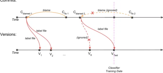
Figure2.1 depicts how commits and files are identified as vulnerable from vulnerability fixing commits. Figure2.1 shows two ‘vulnerability fixing commits’ discovered at different points in time, and depicts how they are used, or left unused for labelling vulnerable instances in training sets at file and commit level. The upper timeline represents commits made over time. The lower timeline shows a series of versions, the files of which are used as the training set (V1 to V9), and testing set (VT est) for file-level prediction at the given ‘training date’. Figure 2.1 shows how files in these versions are identified as containing a vulnerability, as we are about to describe further.
Cf ix1 is a vulnerability fixing commit, identified as linked to a vulnerability in NVD
as described above (and in further detail in Section 6.1). The lines changed by the Cf ix1
are considered to be the vulnerability. Cblamed1 is then identified as a ‘blamed commit’, by
finding the most recent commit (beforeCf ix1) to modify a line fixed by the fixing commit
Cf ix1. We use the version control system (specifically, ‘git blame’ [2] or an equivalent) to
identify Cblamed1 from the modified line inCf ix1. Following the techniques used in previous
work [31,50,71,47], we considerCblamed1 as a ‘vulnerability introducing commit’, or simply
a ‘vulnerable commit’. Because Cf ix1 was made before the ‘training date’, meaning the
vulnerability is known at time of prediction, we labelCblamed1 as vulnerable in the training
set at commit level. At file level for the same ‘training date’, the file containing the line modified inCblamed1 is labelled as vulnerable in VersionsV1andV2, and used in the training
set. A file is considered to be vulnerable until it is fixed by the ‘vulnerability fixing commit’, and only after it is modified by the ‘vulnerability introducing commit’.
On the other hand, the vulnerability fixing commit Cf ix2 is made after the ‘training
date’, meaning that at the time of prediction, the vulnerability may not have been discov-ered, and a researcher performing prediction at that time would have no knowledge of the vulnerability without access to ‘future data’. For this reason, Cf ix2 is not used to label
blamed commit Cblamed2 as vulnerable in the training set at commit level for the given
Figure 2.1: Labelling vulnerable (‘buggy’) instances. Cf ix1 is a vulnerability fixing commit.
A line fixed byCf ix1 was last modified by vulnerable commit Cblamed1, which is considered
vulnerable in the training set at commit level. At file level, the file containing the line in modified inCblamed1 is labelled as vulnerable in VersionsV1 andV2. The vulnerability fixing
commitCf ix2 is made after the ‘training date’, and so is not used to label blamed commit
Cblamed2 or the file modified byCblamed2 in versionV9 as vulnerable in the commit-/file-level
training sets. However, it is used to label the file modified byCblamed2 in thetesting set at
file level, versionVT est.
vulnerability) in the file-level training set for the given ‘training date’. However, Cf ix2 is
used to label the file modified byCblamed2 in the testing set at file level, version VT est.
Following this technique, we label known vulnerable instances in a projects history for a model’s training set (based on a given ‘training date’), and label all possible vulnera-ble instances in the testing set. We then use these labellings to build and evaluate our prediction models.
2.6
Feature extraction
Classification algorithms take as input a set of labelled instances, where each instance is described using a vector offeatures, or attributes of the given commit or file. We choose a set of features over a broad range of categories similar to the ones used in previous work [50, 54, 43,63] for both commit and file levels.
1. Complexity Metrics (i.e. cyclomatic complexity, nesting, lines of code) are a set of features we use for prediction. The intuition behind this kind of features is that complex entities are more likely to be vulnerable. These metrics have been widely used in previous work [63, 43, 42].
2. Code Churn Metrics, such as the number of changes or number of lines added or deleted, have been shown to be some of the most relevant features [56, 44] for pre-diction, and have been extensively used in previous work, both at commit and file level [63, 43, 50].
3. Developer Activity metrics contain features related to the authors of each commit and file (e.g. author contribution). For example, it is possible that authors with a small contribution to the projects to be more prone to adding vulnerabilities, as they are not familiar with the project. These features have been used in previous work [63,31, 73, 50].
4. Keyword features consist in counting how many times specific keywords appear in the commit or file. We use the list of keywords provided in previous work [50]. Some features need to be adapted to be used at different levels of granularity. For example, the commit-level features ‘additions’ and ‘deletions’ listed in Table3.1 are anal-ogous at file-level to the features ‘sum additions’ and ‘sum deletions’. We describe these differences and how we mitigate this threat in Section 3.1.
2.7
Evaluation Measures
To evaluate the performance of the classification models in various aspects, we use four measures, or evaluation metris. In terms of practical use of vulnerability prediction models, we can consider two usage scenarios, i.e., a prediction performance scenario, and a cost effectiveness scenario. In the prediction performance scenario, the goal of prediction models
is to precisely predict as many vulnerabilities as possible. The cost effectiveness scenario aims at minimizing cost for software quality activities such as code review and testing while maximizing high detection rate of vulnerabilities by the quality activities. Thus, vulnerability prediction models often cannot be evaluated by a single measure for both scenarios.
For the prediction performance scenario, we use F1 score [43] since it is computed by
precision and recall together. However,F1score is known as unstable since it varies
depend-ing on probability threshold [56]. For this reason, we use AUROC (Area Under receiver operating characteristic Curve), that is independent from the probability threshold [54].
In terms of cost effectiveness, we use the area under the cost effectiveness curve (AUCEC), which plots the recall against the percentage of lines of code ‘inspected’ [56, 42]. Since AUCEC represents how early vulnerabilities can be detected by inspecting the entire LOC, it does not fairly estimate inspection cost between two projects with different LOC. For this reason, we also use TPR10k (Percentage of vulnerable instances in 10K Lines of Code), similar to the cost effectiveness measure used by Jiang et al. [31].
The F1 score is calculated as the harmonic mean of the precision and recall of a
clas-sifier. Precision measures the number of true positives (tp - correctly predicted buggy instances) out of all predicted buggy instances (true and false positives), and indicates how likely a predicted buggy instance is likely to be an actual buggy instance. Recall measures the number of true positives out of all actual buggy instances (true positives and false negatives), and indicates what portion of the buggy instances were identified by the classifier. F1 can be calculated directly from confusion matrix values as 2tp+2f ptp+f n, where
f p is the number of false positives (instances incorrectly predicted as buggy), and f n is the number of false negatives (instances incorrectly predicted as clean).
AUROC is computed as the area under the receiver operating characteristic curve (ROC curve), which plots the true positive rate (recall) against the false positive rate, and visualizes the tradeoff between true positives and false positives as the threshold for prediction is varied. A randomly guessing classifier would have an AUROC of 0.5, while a perfect classifier would have an AUROC of 1.
Similarly, AUCEC is the area under the cost effectiveness curve, which plots the recall against the percentage of lines of code ‘inspected’. This metric indicates how useful the model is when developers have limited time and resources and can only analyse a specific percentage of the elements flagged as vulnerable by the prediction model. Menzies et al. [42] suggest the use of AUCEC over AUROC as a metric to optimize in the context of defect prediction, in order to locate more vulnerabilities within a smaller amount of code.
The TPR10k metric is similar to the NofB20 metric used in [31], however, because the number of lines of code can vary between the test sets for commit and file level, we use an absolute number (10KLOC), rather than a percentage (20%) in order to facilitate a fair comparison. Based on a developer review rate of 200 LOC/hr (as recommended by Kemerer et al. [33]), 10kLOC would take 50 man hours, or between 1-2 weeks of inspection time.
In this section, we have outlined several key background concepts for vulnerability prediction, including how a prediction model is built using data from a training set, and then evaluated on a testing set. We first discussed how prediction can be designed to emulate a real-world use case by collecting training and testing set data following online prediction methods. We then discussed how the instances in the data are labelled as vulnerable or not vulnerable using information from NVD and the project’s version control history. We outlined the categories of features that are used to represent instances in our data to the classification algorithms. Finally, we discussed several common metrics that are used in the evaluation of the performance of a classification algorithm and detail how they each capture varying aspects of a classifier’s performance.
Chapter 3
Study Design
In order to compare the predictive performance and cost effectiveness of vulnerability prediction at file and commit levels, we build classifiers for both levels of granularity on the same set of projects, using an analogous set of features. We then evaluate the quality of each classifier using the metrics discussed in Section 2.
It is nontrivial to fairly compare file- and commit-level prediction since commits and files do not share a hierarchical relationship. In previous work [54, 43] comparing defect or vulnerability prediction at different levels of granularity that are hierarchically related, such as file and binary levels, a comparison can be made by selecting the set of files that makes up the binary. No such hierarchy or similar subset relationship exists between file and commit levels. Indeed, many of the features extracted, and the entities predicted on are semantically different at file and commit levels. In this section, we describe the major differences between file- and commit-level vulnerability prediction and how we proceed to design a fair comparison between commit and file levels. We start by describing the set of features used to describe each instance for prediction, then describe in detail our technique for selecting training and testing sets for the construction and evaluation of our predictive models. Finally, we discuss the research question which we set out to answer in our experiments.
3.1
Features
Features at file and commit levels are different because files and commits are very different entities. While a file can be considered as a chunk of code that exist in a specific snapshot
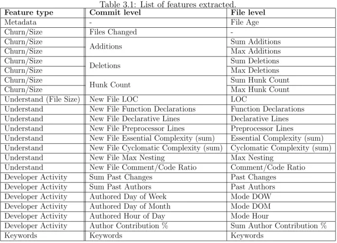
of the software, a commit represent changes made to a software. Some type of features are more easily derived for a file (e.g. complexity metrics) while other types of features are extracted from commit related information (e.g. churn features). In this section, we describe the differences between features we used at file level and commit level. Table 3.1 lists the features for commit and file levels respectively. The features are aligned by row such that features in the same row are roughly analogous at commit and file level. Note that in some cases, one commit-level feature may correspond to multiple file-level features.
3.1.1
Code Churn features
The first set of features listed in Table 3.1 represent code churn metrics at file level, or are representative of commit size at commit level. ’Additions’, and ’deletions’ count the number of added or deleted lines in a commit. To adapt such features at file level, we aggregate such information. For example, we sum the code churn features of all commits that modified the file in the past. Because of the assumption that higher churn (i.e., larger commits) are more likely to be vulnerable, for each file, we also keep the maximum of each attribute associated to past commits.
3.1.2
Developer Activity features
In addition to the above described features, we collect metrics that measure developer activity, similar to those used by previous work [31, 73, 50, 63]. These include the number of past changes, or distinct past authors to a file, the day of week or hour of day the commit was authored, and the percentage of total commits the author has made to the project. Because a file was likely modified at different times, we aggregate the timing features (day of the week, hour of the day, day of the months). For past change and past authors of the file, we sum the number of changes and past authors at the time of the version the file was extracted.
3.1.3
Complexity Metrics
Complexity metrics were collected using the Understand tool [3], which supports the col-lection of various metrics of source code files and projects, and has been used in previous studies for defect and vulnerability prediction, such as Shin et al. [63]. Most of these metrics are easy to obtain at file level for specific version of a project (e.g. max nesting,
Table 3.1: List of features extracted.
Feature type Commit level File level
Metadata - File Age
Churn/Size Files Changed
-Churn/Size
Additions Sum Additions
Churn/Size Max Additions
Churn/Size
Deletions Sum Deletions
Churn/Size Max Deletions
Churn/Size
Hunk Count Sum Hunk Count
Churn/Size Max Hunk Count
Understand (File Size) New File LOC LOC
Understand New File Function Declarations Function Declarations Understand New File Declarative Lines Declarative Lines Understand New File Preprocessor Lines Preprocessor Lines
Understand New File Essential Complexity (sum) Essential Complexity (sum) Understand New File Cyclomatic Complexity (sum) Cyclomatic Complexity (sum) Understand New File Max Nesting Max Nesting
Understand New File Comment/Code Ratio Comment/Code Ratio Developer Activity Sum Past Changes Past Changes
Developer Activity Sum Past Authors Past Authors Developer Activity Authored Day of Week Mode DOW Developer Activity Authored Day of Month Mode DOM Developer Activity Authored Hour of Day Mode Hour
Developer Activity Author Contribution % Sum Author Contribution %
Keywords Keywords Keywords
cyclomatic complexity), but cannot be used to measure the complexity of a commit be-cause they require at least a full function to be computed. Bebe-cause we need to work on complete files, we consider the complexity of the commit as being the complexity of the file after the commit was applied.
We do not collect dependency metrics (for example, FanIn, the number of calls in the project to functions in a file) for scalability reasons. Indeed, it would require applying the tool to the entire project for each commit to measure the number of calls. For the 8 projects under study, it would be equivalent to running Understand more than 600,000 times on complete projects.
3.1.4
Keywords
Finally, we collect counts for a set of keywords at both commit and file level. We use the same set of keywords as used in previous work [50], a list of 68 common C/C++ keywords and common standard library functions. At file level, we count how many times each keyword appears in the file. At commit level, we count how many time each keyword appears in the patch (lines added, lines deleted and context lines) and do not consider the commit message. We did not consider keywords in the commit messages because the same keyword might have a different meaning in the code and the commit message. For example, the keywords ‘for’ in the source code (patch or file) indicates that the code contains a loop. The semantic of this keyword in the patch message is different because these messages are written in plain English. The full list of extracted keywords can be found in AppendixE.
3.2
Training and Test Sets
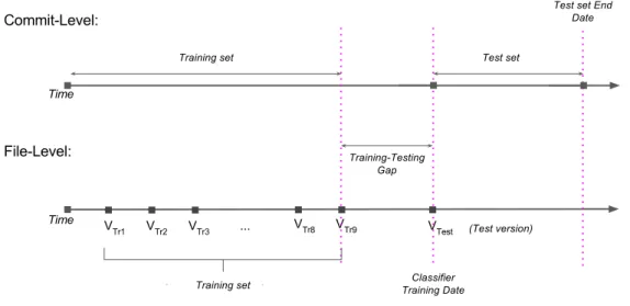
In order to perform a fair comparison between granularity levels, we go to length to ensure we use an analogous set of data for training our file- and commit-level models. Figure 3.1 depicts this process, as described in detail in the following section.
In order to perform an evaluation of the performance classifier, instances are divided into a ‘training’ and ‘testing’ sets at each level, as depicted in Figure3.1. Recall that a testing set of data separate from the data the classifier has been trained on is used to evaluate the classifier, to demonstrate the model’s generalizability to other data, and to ensure that overfitting has not occurred. As mentioned earlier, because we aim to perform ‘online prediction’ in order to simulate real, practical use of vulnerability prediction, traditional classifier evaluation techniques such as ten-fold cross validation are not applicable to our evaluation.
Instead, we split our dataset into training and testing sets based on dates, dedicating a set of past versions (and their files) or commits as a training set, and predict on a later version or set of commits designated as the testing set. In Figure3.1, we see that we align corresponding file-level and commit-level predictions based on a common ‘training date’.
At commit level, similar to [73, 50], we train our classifier on a set of commits from before the training date (the ‘Training set’, as labelled in Figure 3.1, then test on the commits after the training date (the ‘Test set’ as labelled in Figure 3.1). At commit level, following previous work [31, 73], we also exclude a period of early commits from the training set, as early project commits and young projects may have distributions of
Figure 3.1: Training and testing sets for file- and commit-level prediction. The upper timeline depicts the set of commits selected for the training and testing set and used to build and evaluate the commit-level prediction models for the given ‘training date’. The lower timeline depicts a set of versions chosen for the training set (VT r1 to VT r9), and
the version used as the test version (VT est) relative to the ‘training date’. Note that in both cases, we leave an identical ‘training-testing gap before the training date, in order to facilitate a fair comparison.
vulnerabilities and features much different than current commit patterns, and negatively impact prediction performance. Similar to previous work [73], we exclude the first 3 years of a project’s commits for projects older than 6 years, and the first 6 months of commits for projects less than 6 years old. We also exclude the commits made less than 8 months before the testing set from the training set, as these commits are likely to have a greater number of undiscovered vulnerable instances. This period is labelled as the ‘Training-Testing Gap’ in Figure 3.1, and the same gap is used at both commit level and file level. Finally, for the testing set, we exclude 6 months of commit data prior to our last known vulnerability (we have data up until the end of 2015), in order to exclude testing data that has a higher level of undiscovered vulnerable instances.
At file level, we use a similar technique to the next release validation used by Shin et al.[63], which uses several previous releases as a training set, in order to predict on an ‘upcoming’ release. Some key differences are that we use project ’snapshots’ as opposed to releases, and that we do not use ‘future vulnerabilities’ (vulnerabilities discovered after the training date) in the labelling of our training versions, as discussed in Section2.5 and Figure2.1. We take 9 project snapshots (VT r1 toVT r9 in Figure 3.1), with the final project
snapshot falling at the start of the ‘Training-Testing Gap’, in order to correspond with data collected at commit level. For our testing set, we use a snapshot of the project at the ‘training date’, which corresponds to time of the start of the commit-level Test set, as can be seen in Figure3.1.
The ‘Training-Testing Gap’ in Figure3.1is used in order to omit data that has a greater number of undiscovered vulnerable instances. For instances close in time to the training date, fewer vulnerabilities have been discovered as of the training date, because it takes time to discover a vulnerability after it has been introduced. In particular, close to the training date, no ‘real’ vulnerabilities have yet been discovered, so all vulnerabilities in that period are undiscovered vulnerable instances. This issue is further demonstrated in Section6.3.
In summary, training and test sets for both commit and file-level prediction are aligned. Having matching training and test sets for both file and commit level is important to ensure that (1) we use equivalent data to train both commit and file level models and (2) our evaluation of these models is done on the same time period.
Finally, while the technique of withholding data for a ‘Test Set’ is used to evaluate the generalizability of a given predictive model, we also want to test the generalizability of the classifier or prediction algorithm’s performance to other data. In order to do this, we repeat our experiments across 8 different ‘training dates’, keeping file- and commit-level data aligned for each repetition of our experiment. Note that at each date, we build a new prediction model using that date’s training set, and evaluate it on that date’s testing set (at both commit and file level). Since the goal of our study is to systematically compare commit- and file-level vulnerability prediction, we conduct our experiments under various settings. Using different training dates affects the size of training and test sets, feature values, and labels of training sets. If prediction results under various situations show similar trend, it would be more helpful to generalize the conclusion of our experiments.
3.3
Research Question
Using the above described fair comparison, we set out to answer the following research question, with the goal of informing the development of vulnerability prediction towards practical use:
• How do commit-level and file-level ‘online’ vulnerability prediction compare in terms of ‘predictive performance’ (F1 and AUROC) and ‘cost effectiveness’ (AUCEC and
TPR10k)?
Recall that the aforementioned metrics are described in detail in Section 2.7. We divide the metrics into two usage scenarios, a ‘predictive performance’ or ‘classification performance’ scenario, and a ‘cost effectiveness’ scenario. The ‘predictive performance’ metrics measure the quality of prediction given that all predicted positive instances are inspected for vulnerabilities. These metrics may be useful in a security review setting, where all predicted instances are of interest, and resources exist to examine them further. The ‘cost effectiveness’ metrics allow us to compare classification performance based on the number of vulnerabilities found after looking at a given amount of code. In partic-ular, TPR10k was chosen as an evaluation metric in order to make a comparison that is independent of the total number of lines of code, which may vary between file and commit level. These ‘cost effectiveness’ metrics may be useful in a managerial context, when a limited or set amount of review resources are available to inspect code for vulnerabilities, and only the top n predicted lines of code can be examined. Taken together, these metrics provide different insights on the effectiveness of the vulnerability prediction techniques we are evaluating.
In this section, we have discussed in detail the design of our approach for comparing commit-level and file-level vulnerability prediction, highlighting how we design for a fair comparison between the two levels of granularity. We first detailed the set of features used to describe each instance for prediction, and how we choose an analogous set of features at each level of granularity. We then described in detail our technique for selecting analogous training and testing sets at commit and file levels. Finally, we have discussed the research question that we set out to answer in our experiments: how do commit- and file-level vulnerability prediction compare under several different metrics, and different usage scenarios?
Chapter 4
Experimental Setup
We train and evaluate classifiers for 7 different open-source C/C++ projects. For each of those projects, we evaluate on up to 8 different train-test splits (limited in some cases by project age and vulnerability report availability). In the following sections we discuss in detail the experimental setup, parameters, and data we used for our evaluation. We first describe the different projects on which we performed our evaluation, and provide some information on their size and buggy rate. We then detail the classification algo-rithms used in our evaluation, as well as the tuned parameters for each. We discuss the data preprocessing steps we applied to our training data in order to improve classification performance. Finally, we discuss the implementation of the tool used to collect data and perform our evaluation, as well as the runtime of several key steps in data collection and classifier training.
4.1
Projects under study
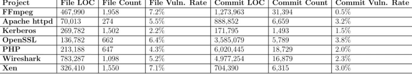
The 7 projects we examine in this study are listed in table 4.1. Columns 2 and 3 indicate the number of files and lines of code as of Jan 1, 2013 in each project. Columns 5 and 6 indicate the number of commits to the project between Jan 1, 2013 and Jul 1, 2015, and the LOC in those commits. Columns 4 and 7 indicate the buggy (vulnerable instance) rate of the project at file and commit level in the aforementioned version and commit period, labelled using data up until the end of 2015. Projects were selected from the set of open-source, C/C++ projects known to contain vulnerabilities in the NVD. eters
Table 4.1: Projects under study.
Project File LOC File Count File Vuln. Rate Commit LOC Commit Count Commit Vuln. Rate FFmpeg 467,990 1,958 7.2% 1,273,963 31,394 0.5% Apache httpd 70,013 274 5.5% 888,852 6,659 3.2% Kerberos 269,782 1,502 2.2% 171,795 1,493 1.5% OpenSSL 136,782 662 6.4% 3,585,079 5,789 3.8% PHP 213,188 647 4.3% 6,020,445 18,729 2.0% Wireshark 783,287 1,098 5.2% 4,977,254 16,879 2.3% Xen 326,410 1,550 7.1% 704,390 6,315 3.0%
Table 4.2: Classifiers under study.
Classifier Tuned parameters Naive Bayes None
Logistic Regression Ridge parameter
Multilayer Perceptron Learning rate, momentum, number of layers/nodes per layer
ADTree Number of boosting iterations
J48 Decision Tree Pruning confidence
Random Forest Number of attributes to randomly investigate
4.2
Classification algorithms and tuning
We evaluate and compare the performance of several commonly used machine learning algorithms on each of our 7 projects. We rely mainly of the implementations of these algorithms as provided by Weka [24], an open-source java implementation of many common machine learning algorithms and related tools. Weka classifier implementations have been used in previous defect prediction work [31]. In order to tune the parameters of each classifier, we randomly select one project and use Weka’s MultiSearch tool, which extends the grid search technique to more than 2 parameters. MultiSearch takes a list of parameters to be tuned and a set of possible values for those parameters (e.g., for numerical values: min, max, step), and evaluates the classifier for each possible combination of those parameters, selecting the set of values that provided the best performance in terms of F1 score. The
list of algorithms used, as well as the parameters tuned, are listed in Table4.2. We tune a separate set of parameters for both file and commit levels because we want the classifiers to perform optimally in both cases. Compared to previous work [50], we do not show results for Support Vector Machine (SVM) because, for all projects, all metrics, and both levels of granularity, this classifier performed poorly in our experimental setting.
4.3
Preprocessing steps
Before training our classifiers, we apply a number of preprocessing steps to the training data in order to improve classification performance. Vulnerability prediction suffers to a significant degree from imbalanced data, as can be seen in Table4.1, where positive instance rates are at 7.2%, and lower at file level, and 3.8% or lower at commit level. In addition, imbalanced data in the training set is made worse when building and evaluating a model using online prediction [73]. Because of this, we use a combination of undersampling of the negative (majority) class, and SMOTE (synthetic minority oversampling) on the positive class, as performed in [10]. In this way, the training data is resampled to contain an artificially higher number of positive instances. We tune the extent undersampling for file and commit levels individually by taking the highest F1 score on a randomly selected
project, averaged over all classifiers using their default parameters. Parameters for each of the classifiers were tuned after choosing the optimal sampling parameters.
Finally, before training each of the classifiers, we perform attribute selection on the training data, using forward feature selection in order to select a subset of features that provides a high information gain on the instances in the training data. We perform at-tribute selection separately for commit and file levels, giving us a separate set of optimized attributes at each level. This subset of features is then used to train and evaluate the classifiers.
4.4
Implementation and Runtime
In order to implement our evaluation, we developed a series of scripts, built primarily in python, to collect feature and vulnerability fixing data, produce feature vectors and la-belling for given training dates, and preprocess, train, test, and evaluate the classification models. In this section, we discuss the implementation details and high-level functionality of the tool we built to perform and evaluate vulnerability prediction at commit and file levels. We first collect data on commits, files, and vulnerabilities from the project source repositories and NVD for calculating feature vectors and labellings. We thengenerate train-ing and testtrain-ing sets, calculattrain-ing feature vectors and correct labelltrain-ings for a set of traintrain-ing date parameters. Finally, we train and test our classification models, also preprocessing data and calculating evaluation metrics in these steps.
Our scripts first collect data from NVD and project source repositories for labelling instances and calculating features. NVD provides the contents of its database in a series
of XML documents, which we parse in order to obtain vulnerability information. We then traverse each of our projects’ commit histories using the projects’ version control system, identifying fixing commits, finding vulnerability introducing commits (as described in Sec-tion 2.5), and recording data for the calculation of features. The relevant data is stored in an SQLite database for more convenient access for calculating training and testing sets. The data includes the commit identifiers, commit date, files changed, vulnerability fix-ing information, meta information used in calculatfix-ing features, and blame information for identifying vulnerability introducing commits and vulnerable files. We separately gener-ate complexity metrics using the Understand C++ tool [3], which are incorporated when calculating feature vectors for our training and testing sets.
Once the data has been collected and stored to our SQLite database, we then generate training and testing sets. In order to do this, we query the database for a given a training date and granularity level to calculate the feature vectors and labels for the training and testing sets. As necessary, we aggregate commit-related metrics to their matching file-level metrics, and vice versa when calculating the feature vectors. When aggregating commit-level features for a file, we examine the set of commits that have previously modified that file. When aggregating file-level features to a commit, we examine the set of files modified by that commit as of the date the commit was made. We also have scripts for automatically generating configuration parameters (start and end for training and testing sets) for a given training date. We also incorporate features calculated separately using the Understand C++ tool here.
Finally we use a series of scripts, written in bash and python, in order totrain and test our classification models, using classification algorithms implemented in Weka [24]. We first perform preprocessing on the training data (as described above in Section 4.3). We then train each of our classifiers using each of our classification algorithms, and test the models by using them to predict on the data in the testing sets Finally, we calculate the performance metrics based on the predicted results.
We ran our experiments on a 3.3GHz E5-1660 shared server with 12 logical cores, 6 physical cores, and 32GB memory. Complexity metrics from Understand C++ were run on a 2.93GHz Quad Core Intel i7 machine with and 12GB memory, dedicated for Understand C++ for the duration of the data collection process. The runtime for the entire process for all projects was on the order of weeks. The majority of that runtime cost was the collection of complexity features using Understand C++. We break down the total runtime cost into the costs forcollecting data, generating training and testing sets, and training and testing each below. For each stage, we first report the total runtime cost, then break down the runtime costs of the steps that make up each stage.
Collecting data took on the order of weeks. Again, the majority of this cost was caused by the collection of complexity metrics with Understand C++, which took on the order of days to weeks for each project. We note that we calculate metrics for changed files after each commit in a project’s history in order to generate complexity metrics with Understand C++. To the best of our knowledge, Understand C++ does not support the incremental analysis of changes below the level of a file. We ran multiple projects in parallel, with the longest project taking an estimated 2 weeks to complete. Collecting other features for each commit from the project repositories took approximately 4 hours for all projects, based on timing information recorded in log files. Identifying vulnerability fixing commits, including parsing NVD data and dumped history of commit log messages, and identifying vulnerability introducing commits took under an hour for all projects. Outputting the commit log messages and commit data from the project’s version control system for further parsing took on the order of a day for the largest projects.
Generating training and testing sets for each project-prediction-date combination took under a day. Calculating feature vectors from previously collected data for all 8 training dates and 7 projects took approximately 8 hours for commit-level features, and approxi-mately 2 hours for file-level features. Calculating labels from previously collected data for all 8 training dates and 7 projects took just under 2 hours each for commit and file levels. Training and testing each of the 6 classifiers for 8 training dates and 7 projects took on the order of days. Training each individual classification model took on the order of minutes for most classifiers, except for the Multilayer Perceptron models, which took on the order of hours to train. Testing and evaluating each classifier takes on the order of minutes to test. Again, the whole process of our evaluation, from collecting data to training and testing took on the order of weeks.
In this section, we have discussed our experimental setup, projects, parameters, im-plementation and runtime. We have described the projects and classification algorithms used, and the preprocessing steps applied in our evaluation. Finally, we have discussed the implementation and runtime of the tool used to perform the evaluation.
Chapter 5
Findings
In this project, we seek to compare vulnerability prediction at commit level with predic-tion at file level under different usage scenarios. We set out to compare commit-level and file-level prediction under two usage scenarios, ‘prediction performance’, and ‘cost effec-tiveness’. In order to do so, we have performed online vulnerability prediction across 7 different projects, using 6 different classifiers, and using 8 different training dates (for a total of 336 runs per level). Here we present a comparison of the series of runs using each project and classifier. We find that generally file-level prediction outperforms commit-level prediction for most projects, especially as measured by F1, and TPR10k metrics. There
are some notable exceptions, however. In particular, commit-level prediction often outper-forms file-level prediction in AUROC and AUCEC metrics for the PHP project. Finally, we show the ROC and CEC curves for specific prediction runs, and demonstrate that below certain thresholds, commit level can occasionally outperform file level in both the ROC (‘prediction performance’) curve, and the CEC (‘cost effectiveness’) curve.
5.1
Comparison of prediction performance and cost
effectiveness
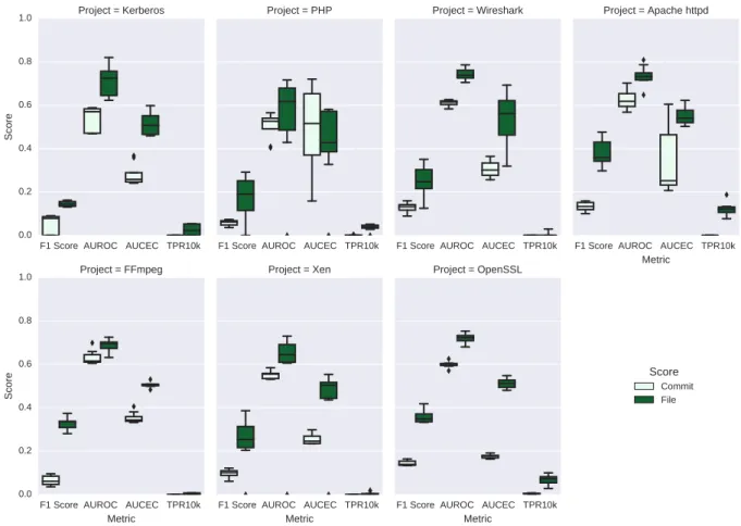
Figure5.1 shows the box plots for each classification performance metric, comparing com-mit level and file level across each of the 7 projects, for the Naive Bayes classifier. We select the Naive Bayes Classifier to show here, as it achieves the highest averageF1 score for all
projects in the Jan 2013 test date at file level, but similar plots of other classifiers can be seen in Appendix A. The y-axes of the box plots measure the scores for each metric. The
plot is split up into 7 sections, depicting the performance within each project, and each project has four pairs of box plots, each comparing commit-level and file-level performance for the same metric. The four metrics presented on the plot areF1 score, AUROC, AUCEC,
and TPR10k, in that order. For all measures, a higher score indicates better performance. Each box represents the 8 runs for each test date at that repo/classifier setup. On each box plot, the minimum and maximum results (excluding outliers) are represented by the extremities of the tails. Outlier results are represented by a dot. The top and bottom lines in a box of each plot show performance results at first and third quartiles respectively, while the solid line in the box represents the median. Similar box plots for each of the other 6 classifiers can be found in Appendix A.
In each of the projects, comparing the median performance of each metric at commit level and file level, we find that, except in certain cases discussed below (for example the AUROC score for the PHP project in Figure5.1, file-level prediction outperforms commit-level prediction. As such, we report the following finding:
File-level prediction tends to outperform commit-level prediction in both ‘predictive per-formance’ and ‘cost effectiveness’ metrics, across most projects and classifiers.
Our results indicate that despite being a finer granularity, commit-level prediction is not more cost effective than file-level prediction for most projects and classifiers. Cf. Posnett et al. [54], who find that when comparing the hierarchically-related granularity levels of file and package level, the finer-grained file-level vulnerability classification can be shown to be more cost effective. However, commit- and file-level prediction are not hierarchically related in the same way; as discussed in Section 3, there are differences in the meanings and distributions of corresponding prediction features.
However, we also find that for F1 and TPR10k, consistently have median scores that
are quite low. For no classifier/project pair does the median F1 score reach above 0.5,
similarly most median TPR10k scores are around 0.1 or lower. These results correspond with Morrison et al.’s [43] discussion that the current state of the art in vulnerability prediction is not effective enough that it is widely used in industry. However, based on our results, for most projects, focusing on the development of features and techniques for file-level prediction would be more promising.
Figure 5.1: Naive Bayes performances by project, level, and metric.
5.2
Cases with higher commit-level performance
As discussed above, while file-level prediction tends to outperform commit-level prediction for most projects/classifiers and metrics. However, in this section, we highlight cases where commit-level prediction outperforms file-level prediction. Again, we compare median values in the box plots in Figure5.1and AppendixA. Most notably, the PHP project consistently has stronger median AUROC scores at commit level across 5 of the 6 classifiers, and has stronger median AUCEC scores at commit level for 4 of the 6 classifiers, Random Forest, J48, and ADTree. PHP also has a higher F1 score at commit level for the J48 classifier.
Additionally, Apache httpd and OpenSSL achieve higher median AUCEC scores at commit level with 2 classifiers (Multilayer Perceptron and Logistic Regression), while Xen has
a higher median AUROC score with 3 classifiers (ADTree, Multilayer Perceptron, and Logistic Regression).
Note also the J48 classifier, which at file level had the lowest averageF1 score across all
projects for the Jan 2013 test date, while at commit level had the second highest average F1 score across projects for the same date. This classifier also had the highest number
of projects which had higher scores at commit level based on the AUCEC, AUROC or F1 metrics. As mentioned briefly above, the J48 classifier had higher median
commit-level scores for the following project/metric combinations: PHP and Apache httpd for the AUCEC metric; PHP, Apache httpd, OpenSSL, Kerberos, and Wireshark for the AUROC metric, and PHP for the F1 score.
Based on these cases, in which commit-level prediction sometimes outperforms file-level prediction under certain metrics and for certain projects, we report the following findings:
For certain projects, particularly PHP, and for certain classifiers, particularly J48, AUROC and AUCEC performance at commit level may be comparable to, or better than, performance at file level.
In these cases, for these projects, and using these classifiers, it may be beneficial to perform vulnerability prediction at commit level rather than file level, depending on the usage scenario, and more specifically, metric, that the user is interested in optimizing.
5.3
AUROC vs. AUCEC
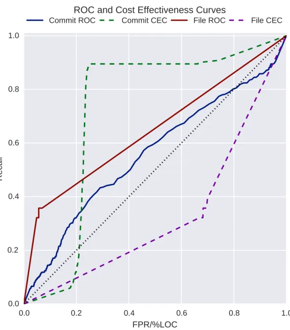
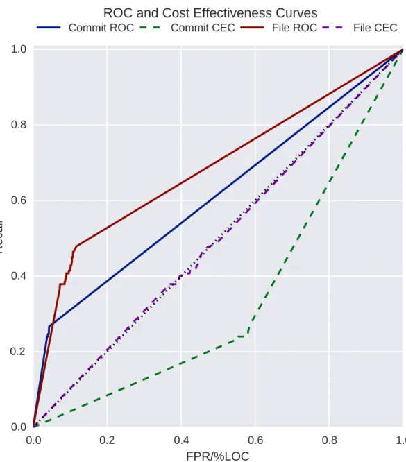
Figures 5.2 and 5.3 show the ROC and CEC curves at commit and file levels for the Naive Bayes classifier using the Jan 2013 test date, and for the PHP and FFmpeg projects respectively. There are 4 curves in total on each plot, two curves plotting the ROC and CEC curves at commit level, and two curves plotting the same at file level. For all curves, the y-axis value represents the true positive rate, or recall. The recall is measured as the number of true positive predictions over the total number of vulnerable instances. For ROC curves, represented on these plots by solid lines, the x-axis of the plot indicates the false positive rate (number of false positives over total number of non-vulnerable instances). The dotted black line represents the ROC curve of a classifier which randomly predicts instances as buggy or clean. On the other hand, for the CEC curves, represented on these plots by dashed lines, the x-axis represents the total percentage of lines of code of
all instances predicted as vulnerable. For both of these values, the curve is calculated as the prediction threshold is brought from 1 (accepting instances only with 100% predicted certainty) to 0 (accepting all instances). At each threshold level, the x and y-axis values are calculated and plotted based on the predicted probability of being vulnerable as assigned by the classifier.
Note that in some curves, sections of the curve appear perfectly linear. In these cases, all of the instances (or lines of code) in the linear section of the curve were