A Constrained Optimization Approach to
Dynamic State Estimation for Power Systems
including PMU Measurements
Liang Hu, Zidong Wang, Izaz Rahman and Xiaohui Liu
Abstract—In this paper, a hybrid filter algorithm is developed to deal with the state estimation problem for power systems by taking into account the impact from the phasor measurement units (PMU). Our aim is to include PMU measurements when designing the dynamic state estimators for power systems with traditional measurements. Also, as data dropouts inevitably occur in the transmission channels of traditional measurements from the meters to the control centre, the missing measurement phenomenon is also tackled in the state estimator design. In the framework of extended Kalman filter (EKF) algorithm, the PMU measurements are treated as inequality constraints on the states with the aid of the statistical criterion, and then the addressed state estimation problem becomes a constrained optimization one based on the probability-maximization method. The resulting constrained optimization problem is then solved by using the particle swarm optimization (PSO) algorithm together with the penalty function approach. The proposed algorithm is applied to estimate the states of the power systems with both traditional and PMU measurements in the presence of probabilistic data missing phenomenon. Extensive simulations are carried out on the IEEE 14-bus test system and it is shown that the proposed algorithm gives much improved estimation performances over the traditional EKF method.
Index Terms—Power systems, state estimation, extended Kalman filter, missing measurements, particle swarm optimiza-tion, constrained optimization
NOMENCLATURE
k Time index.
k|k−1 Time index for prediction from instantk−1to k. k|k Time index for update at instantk.
tj The line connecting nodestandj.
tj0 tside (to the ground) of the line connecting nodes tandj.
r andi Real and imaginary component. N Total number of bus nodes of interest.
M Total number of PMUs.
nv Total number of voltage meters.
np Total number of power meters at the nodes. nf Total number of power meters at the lines.
Ns The set of bus numbers directly connected to nodes. tjl Thelth bus directly connected to busj.
I. INTRODUCTION
State estimation (SE) has long been one of the fundamental problems in the research on power systems. Traditional SE
ap-This work was supported in part by the Engineering and Physical Sciences Research Council (EPSRC) of the U.K. under Grant GR/S27658/01, the Royal Society of the U.K., and the Alexander von Humboldt Foundation of Germany. L. Hu, Z. Wang, I. Rahman and X. Liu are with the Department of Information Systems and Computing, Brunel University, Uxbridge, Middlesex, UB8 3PH, United Kingdom. (Email:[email protected])
proach is typically static where the single-scan weighted least-squares estimators are adopted [1]. Static SE method exhibits the features of fast convergence and easy implementation, but it suffers from the accuracy problems since the dynamics of the power system is ignored.
With rapid development of the sensing techniques, online monitoring has recently become popular which gives rise to the renewed research interests on the design of the dynamic state estimator (DSE). Comparing with the static state estimation scheme, the DSE is capable of achieving better estimation accuracy since more information about the state evolution is utilized. Another advantage of the DSE is its potential ability to provide prediction database that could be adopted as a set of pseudo-measurements in case of missing data or meter outages in the power grids.
Note that the missing data phenomenon constitutes one of the major concerns in state estimation for power systems since data dropouts inevitably occur in the transmission channels of traditional measurements from the meters to the control centre. As discussed in [10], [16], [19], the communication constraints (e.g. limited bandwidth) have inevitably led to network-induced phenomena such as random communication delays and missing measurements. As for missing measure-ments, a conventional way is to treat them as normal bad data
withoutin-depth characterization of the dropouts. The robust optimal placement approach of PMUs has been proposed in [8] to increase the reliability of the system in case of a random failure of any PMU. Very recently, the missing measurement problem has been tackled in [16], [17] where a certain stochastic variable is involved in the estimator, and this renders the difficulties in the implementation. In our paper, instead of the hardware deployment, a software algorithm is developed to mitigate the effect of missing measurements through modifying the traditional DSE approaches.
On the other hand, advanced techniques for synchronized phasor measurements have recently been applied in power systems. Different from traditional SCADA systems, where the magnitude of the nodal voltage can be measured directly, PMUs are capable to measure both the magnitude and the phase of nodal voltages. And due to their intrinsic advantages, the phasor measurement units (PMU) have made it possible to measure the system states in a more accurate and timely way as compared with the traditional measurements. Unfortunately, for economic reasons, it is not affordable to replace all the RTUs with PMUs in the foreseeable future [13], [20]. In other words, only partial states could be measured directly
by PMUs and the rest would have to be estimated by using the conventional RTUs. As such, an emerging research issue is how to integrate PMU measurements into traditional SE algorithms, and this issue has started to gain some initial research attention, see [3], [13], [14], [20], [22]. It should be noted that all the corresponding results available in the literature have been concerned with static SE problems, and the DSE problem in the presence of partial PMU involvements remains as a challenging topic of research [11]. This situation motivates our current investigation.
The main purpose of the present research is to design dynamic state estimators for power systems by making one of the first attempts to solve the aforementioned two challenging problems, i.e., 1) how to account for the probabilistic missing data phenomenon? 2) how to include the PMU measurements in the state estimator design? In this paper, the phenomenon of missing measurements is assumed to occur in a random way and the missing probability for each channel is governed by an individual random variable satisfying a certain probability distribution over the interval[0,1]. The impact of missing mea-surements on the overall estimation performance is considered when designing the estimator. On the other hand, to incorpo-rate the PMU measurements into the widely used extended Kalman filter (EKF) algorithm, the PMU measurements are characterized via a set of inequality constraints based on the well-known3-sigma rule of the Gaussian distribution, and then the EKF problem with state constraints becomes a constrained optimization problem that can be effectively solved by the particle swarming optimization (PSO) algorithm. As PSO has been developed primarily as an unconstrained optimization method, the penalty function approach is utilized to convert the constrained optimization problem into an unconstrained one.
In this paper, a hybrid EKF and PSO algorithm is developed to estimate the states of power system. The main contribution of this paper is threefold. 1) A new dynamic state estimation scheme is first proposed to improve the estimation performance of power system including PMU measurements. Such a scheme has the advantages of being scalable to the numbers of the installed PMUs and of being compatible with existing DSE software. 2) Practical issues of missing measurements in com-munication network are investigated thoroughly and a mod-ified EKF algorithm is developed which is insensitive to the measurement unreliability in terms of acceptable probability. 3) Extensive comparative experiments have been implemented based on different missing rates of the RTU measurements and it is confirmed that our proposed estimation algorithm provides better performance than the traditional EKF in the presence of the missing measurements.
Notation The notation used here is fairly standard except where otherwise stated. Im,1denotes them-dimensional
vec-tor with all elements equal to1. For given matricesAandB
with the same dimension, ◦ is the Hadamard product defined as [A◦B]ij = [Aij ×Bij]. E{x} stands for the expectation
of the stochastic variable x. |C| describes the determinants of a square matrix C. diag{· · · } and diagn{∗} stand for a block-diagonal matrix anddiag{
n z }| {
∗,· · ·,∗}, respectively.
II. PROBLEMFORMULATION ANDPRELIMINARIES
A. System Model with Missing RTU Measurements
In this paper, the power network is assumed to operate a-mong quasi-steady states and such kind of steady-state dynam-ics is typically different from the transient ones generated by the electro-mechanical power systems. The following model for representing the slow system dynamics of N buses has been reported in the past [4-6] and [17,18] :
x(k+ 1)−u=A(x(k)−u) +ω(k) (1) where the state x(k) ∈ R2N is the vector of the
real parts and the imaginary parts of the voltages at all buses in the rectangular form, that is, x(k) =
xr,1(k)xr,2(k) · · · xr,N(k)xi,1(k)xi,2(k) · · · xi,N(k) T
, andu∈R2N is the trend behavior of the state trajectory.ω(k)
is a Gaussian sequence with zero mean and covariance matrix
W(k). A represents how fast the transitions between states are. The initial value of statex(0)is a white Gaussian noise with mean value x¯(0)and covariance matrix Σ(0|0).
In the state transition equation, there are three parameters to be determined, namely, A, W andu. The parameters can be obtained by online or offline methods.
For the purpose of simplicity, defineB:=I−A, then (1) can be rewritten in the following compact form:
x(k+ 1) =Ax(k) +Bu+ω(k). (2) The ideal measurement (without missing phenomena)
z(r)(k)∈
Rm collected by RTUs is given as follows z(r)(k) = [VT(k) PT(k) QT(k) Pf T(k) Qf T(k)]T.
Assuming the general two-port π-model for the network branches, the explicit element for each aforementioned mea-surement is given as follows (the symbol of time instant,k, is omitted for brevity):
Vs= q x2 r,s+x2i,s Ps=xr,s X j∈Ns (Gsjxr,j−Bsjxi,j) +xi,s X j∈Ns (Gsjxi,j+Bsjxr,j) Qs=xi,s X j∈Ns (Gsjxr,j−Bsjxi,j) −xr,s X j∈Ns (Gsjxi,j+Bsjxr,j) Psf :=Ptjf = (x2r,t+x2i,t)(gtj0+gtj)−xr,txr,jgtj
−xi,txi,jgtj−xi,txr,jbtj+xr,txi,jbtj Qfs :=Qftj =−(x2r,t+xi,t2 )(btj0+btj)−xi,txr,jgtj
+xr,txi,jgtj+xr,txr,jbtj+xi,txi,jbtj
(3)
where V(k) = [V1(k) V2(k) · · · Vnv(k)]
T denotes the
bus voltage magnitude measurements, P(k) = [P1(k)P2(k)
· · · Pnp(k)]
T andQ(k) = [Q
1(k)Q2(k) · · · Qnp(k)]
T stand
for the real and reactive bus power injections measurements, and Pf(k) = [Pf 1(k) P f 2(k) · · · P f nl(k)] T and Qf(k) =
[Qf1(k) Qf2(k) · · · Qf nl(k)]
T are the real and reactive
trans-mission line power flows, respectively.Gsj+jBsj is thesjth
element of the complex bus admittance matrix, gtj+jbtj is
the admittance of the series branch connecting bus t and j,
gtj0+jbtj0 is the half admittance of the shunt branch of the
line collecting bus t andj in theπ-model circuit, and Ns is
the set of bus numbers which are directly connected to buss. Taking the measurement noise into consideration, z(r)(k)
can be rewritten as the following compact form
z(r)(k) =h(x(k)) +v1(k) (4)
The nonlinear function h(x)is given as follows:
h(x(k)) = [VT(k), PT(k), QT(k), Pf T(k), Qf T(k)]T,
where the variablesV(k),P(k),Q(k),Pf(k)andQf(k)are
defined in (3). v1(k)is the RTU measurement noise which is
also a Gaussian noise with zero mean and covariance matrix
R1(k). Assume ω(k) and v1(k) are uncorrelated with x(0)
and with each other.
Considering missing measurements, theactualmeasurement
z(k)is described by
z(k) = Ξ(k)h(x(k)) +v1(k) (5)
where Ξ(k) = diag{γ1(k), γ2(k),· · ·, γm(k)} with γi(k)
(i = 1,2,· · ·, m) being munrelated random variables. Ξ(k)
is also unrelated with ω(k), v1(k) andx(0). Furthermore, it
is assumed that the stochastic variable γi(k) is a
Bernoulli-distributed white noise sequence taking values on0or1with: Prob{γi(k) = 0}= 1−µi(k), Prob{γi(k) = 1}=µi(k)
where the value of Prob{γi(k) = 0}is also called the missing
rate of theith measurement.
In RTU measurements, one bus is usually chosen as the reference bus for all the other buses to obtain the relative phase angles, while in PMU measurements, all PMU measurements provide the direct phase angles with respect to the time refer-ence provided by the GPS system. In this paper, we use both RTU and PMU measurements, and therefore all the bus phase angles are relative to the reference dictated by the GPS [13]. As a result, no reference buses are needed. Traditionally, the phasor angles and magnitudes are treated separately as state variables, whereas an alternative representation (i.e. the real and imaginary partsof the bus voltages) (see [4]) is adopted as state variables in this paper.
B. PMU Measurements and Inequality Constraints
In this paper, both the state variables and measured variables are in the rectangular form, which makes a linear PMU measurement model. Assume that the lth PMU is installed at busj, and the measurementz(lp)∈R2(1+Nj)can be described
as follows zl(p)=h zr,j(p) z (p) i,j z (p) r,tj1 z (p) i,tj1 · · · z (p) r,tjNl z (p) i,tjNl iT .
To be more specific, the voltage measurement in the above vector is given as follows
zr,j(p)=xr,j, z
(p)
i,j =xi,j (6)
The current measurement of the line collecting the bus j
andtis as follows
zr,jt(p) = xr,lgjt0−xi,jbjt0+ (xr,j−xr,t)gjt−(xi,j−xi,t)bjt, zi,jt(p) = xi,lgjt0+xr,jbjt0+ (xi,j−xi,t)gjt+ (xr,j−xr,t)bjt.
Considering the measurement noise, the PMU measurements can be presented in the following compact vector form:
z(p)(k) =H(p)x(k) +v2(k) (7)
wherez(p) is the PMU measurement vector, andv
2(k)is the
PMU measurement noise, which is also a Gaussian noise with zero mean and covariance matrixR2(k).H(p)can be obtained
directly from PMU configurations, and it can be found that the measurementz(p)(k)is linearly related to the statex(k).
A seemingly natural idea is to treat the PMU measurements as an additional set similar to the RTU measurements. Note the fact reported in [3], [13], that the standard deviation of the errors of PMU measurements is one to two order magnitude less than the one of traditional RTU measurements. Unfortunately, since the PMU measurements are much more accurate than the RTU measurements, including these two kinds of measurements in the estimation process often results in ill-conditioned filtering procedure due primarily to the low covariance matrix for the PMU measurement noises.
AsR2(k)is always a real symmetric matrix, we can find
a transformation matrixM(k)of appropriate dimension such that the matrix M(k)R2(k)MT(k)is diagonal. Accordingly,
we can obtain the following equation from (7):
M(k)z(p)(k) =M(k)H(p)xp(k) +M(k)v2(k) (8)
where M(k)v2(k) is still a Gaussian noise with zero mean
and covariance matrixM(k)R2(k)MT(k).
Based on the well-known 3-sigma rule of Gaussian distri-bution, we can conclude that the following inequality sets are satisfied with probability99.7%:
−3 ˜R2(k)≤M(k)z(p)(k)−M(k)H(p)xp(k)≤3 ˜R2(k) (9)
whereR˜2(k) :=M(k)R2(k)MT(k)Im1,1. From the
perspec-tive of engineering applications, it is reasonable to assume that the above inequality sets are satisfied all the time. So far, we have characterized the PMU measurements by a set of inequality constraints on the states for the power system.
III. FILTERSCHEMES
A. EKF Design for the System with RTU Measurements
In this subsection, we first introduce the EKF approach to estimating the system state for the system (2) with missing measurements (5). The EKF is of the following form:
ˆ
x(k|k−1) =Axˆ(k−1|k−1) +Bu
ˆ
x(k|k) = ˆx(k|k−1) +K(k)[z(k)−Ξ(¯ k)h(ˆx(k|k−1))]
where xˆ(k|k) is the estimate of x(k) at time instant k
with xˆ(0|0) = ¯x(0), and xˆ(k|k−1) is the one-step pre-diction of x(k) at time k−1. K(k) is the filter gain to be determined at time instant k, and Ξ(¯ k) := E{Ξ(k)} =
the covariance matrices of, respectively, the one-step predic-tion error and the filtering error defined by
˜
x(k|k−1) =x(k)−xˆ(k|k−1), x˜(k|k) =x(k)−xˆ(k|k), P(k|k−1) =E{x˜(k|k−1)˜x(k|k−1)T},
P(k|k) =E{x˜(k|k)˜x(k|k)T}.
Denoting H(k) = ∂h∂x(x((kk)))
x(k)=ˆx(k|k−1), the filter gain
K(k) can be obtained by using the following recursive al-gorithm: P(k|k−1) = AP(k−1|k−1)AT+W(k−1) (10) P(k|k) = [I−K(k)¯Ξ(k)H(k)]P−1(k|k−1) (11) S(k) = Ξ(˜ k)◦(h(ˆx(k|k−1))hT(ˆx(k|k−1))) +˜Ξ(k)◦(H(k)P(k|k−1)HT(k)) +R(k) +¯Ξ(k)H(k)P(k|k−1)HT(k)¯Ξ(k) (12) K(k) = P(k|k−1)HT(k)¯Ξ(k)S−1(k) (13) whereΞ(˜ k) :=diag{µ˜1(k),µ˜2(k), . . . ,µ˜m(k)} withµ˜i(k) = µi(k)(1−µi(k))(i= 1,2, . . . , m).
Remark 1: In this paper, the exact occurrence time for the randomly missing measurements is not required to be exactly known, and this reflects the practical situation in power system. Nonetheless, the statistical law (i.e., the first-and second- order of moments) of the rfirst-andom occurrence of missing measurements is needed in the filter design, where the statistical law could be obtained through statistic tests.
Remark 2: There are mainly two kinds of DSE paradigms in power system state estimation. These two paradigms differ from each other in system dynamics model and time scale. In one paradigm (see e.g. [5], [6], [18] and the references therein) called forecasting-aided state estimation, the bus voltages are chosen as state variables and a succession of the quasi steady-states is assumed to evolve in time. Therefore, a dynamic mod-el is adopted to describe the slow time evolution of the quasi steady-state. In the other paradigm (see e.g. [7], [9] and the references therein), rotor angles and rotor speeds of generators are chosen as state variables, and the classic dynamic model of generators is considered. The DSE of such a paradigm is concerned with the low frequency electromechnical dynamics.
B. The Probability-Maximum Method
For the constrained estimation problem, it is difficult to incorporate the inequality/equality constraint of system states into traditional EKF estimator. Fortunately, the probability-maximum method has been successfully exploited in [15] to convert the constrained estimation problem into a constrained optimization one after each step of the EKF algorithm and, therefore, this method is chosen to handle the constrained EKF problem in this paper.
For presentation conciseness, the notation for time instant,
k, is omitted in this subsection. It is known from [2] that, based on the Kalman filter theory, the state estimate ofxmaximizes the conditional probability density
P(x|Z) = (2π)−
n
2|P|−12exp{−1
2(x−x¯)
TP−1(x−x¯)} (14)
where n is the dimension of x, P is the covariance of the Kalman filter estimate, Z , {z(0), z(1), . . . , z(k)} denotes the set of measurements available at time instant 0,1, . . . , k, andx¯ is the conditional mean ofxgivenZ.
The constrained EKF can be derived by finding an estimate
ˆ
xsuch that the conditional probability P(ˆx|Z)is maximized
andxˆsatisfies the constraint (9). Since maximizingP(ˆx|Z)is
equivalent to maximizing its natural logarithm, the problem to be solved can be expressed as
max lnP(ˆx|Y)⇒min(ˆx−x¯)TP−1(ˆx−x¯)
subject to−3 ˜R2≤M z(p)−M H(p)Cxˆ≤3 ˜R2.
(15) So far, the constrained state estimation problem has been converted into an equivalent constrained optimization problem that can be solved after each time step of the EKF algorithm. As is impossible to develop a deterministic method for the constrained nonlinear optimization problem (15) in the global optimization category, we adopt the PSO algorithm, which is a popular evolutionary algorithm in solving the nonlinear optimization problem.
IV. PSOFORCONSTRAINEDOPTIMIZATIONPROBLEM
Particle Swarm optimization (PSO) is a metaheuristic that optimizes a problem by iteratively searching in a large s-paces of candidate solutions [12]. In PSO, a population of candidate solutions (called as particles) moves in the search space according to two simple mathematic formulae over the particle’s position and velocity. More specifically, each particle’s movement is influenced by its local best known position and also the best known positions, which are updated by other particles, in the search space. By such an iterate approach, the swarm of the particles moves towards the best solutions. The velocity and position of the particle at the next iteration are updated according to the following equations:
vi(s+ 1) =ωvi(s) +c1r1(pi(s)−xi(s)) +c2r2(pg(s)−xi(s)) xi(s+ 1) =xi(s) +vi(s+ 1) (16)
wherexi(s) = [xi1(s), . . . , xid(s)],xi(s)is the position of the ith particle at thesth iteration, andxi(s)∈[xmin,n, xmax,n],
withxmin,nandxmax,nbeing the lower and the upper bounds
for all particles’ positions.vi(s) = [vi1(s), . . . , vid(s)], vi(s)
is the velocity of theith particle at the sth iteration. ω is the inertia weight,c1 andc2 are called acceleration coefficients,
namely, cognitive and social parameters, respectively. r1 and
r2are two uniform random number samples from[0,1].pi(s)
is the local best position encountered byith particle at thesth iteration, andpg(s)is the global best position in the swarm at
thesth iteration.
PSO has been successfully applied to various optimization problems. As to constrained optimization problem, PSO is still valid with the aid of the popular constraint-handling technique: the penalty function approach. By using the penalty function approach, a constrained optimization problem can be converted into a corresponding unconstrained optimization one by adding a penalty term to the original objective function [21].
TABLE I
THE TREND VOLTAGE AT NORMAL STATES
Bus 1 2 3 4 5 6 7 8 9 10 11 12 13 14 Real Parts 1.0600 1.0368 0.9609 0.9858 0.9958 1.0016 1.0022 1.0270 0.9827 0.9769 0.9850 0.9806 0.9755 0.9552 Imaginary Parts 0 0.0943 0.2173 0.1821 0.1563 0.2694 0.2512 0.2643 0.2743 0.2744 0.2724 0.2759 0.2748 0.2812 0 5 10 15 20 0.98 0.99 1 1.01 1.02 1.03 1.04 1.05 1.06 1.07
the actual state
the estimate by traditional EKF the estimate by our proposed EKF
0 5 10 15 20 −0.05 −0.04 −0.03 −0.02 −0.01 0 0.01 0.02 0.03 0.04
the actual state
the estimate by traditional EKF the estimate by our proposed EKF
(a) The real part. (b) The imaginary part.
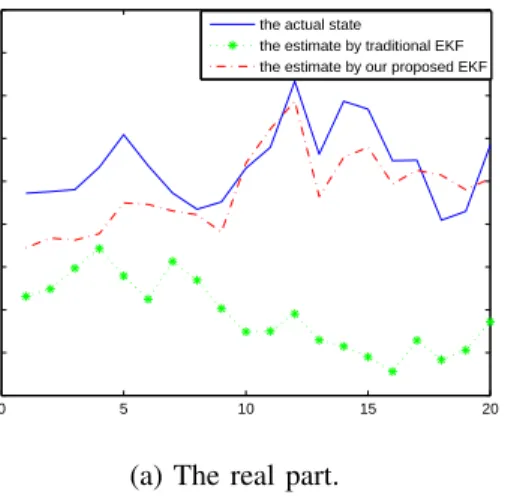
Fig. 1. The estimated states of bus2from the traditional EKF and our proposed EKF
0 5 10 15 20 0.97 0.98 0.99 1 1.01 1.02 1.03 1.04 1.05 1.06
the actual state
the estimate by traditional EKF the estimate by our proposed EKF
0 5 10 15 20 −0.02 0 0.02 0.04 0.06 0.08 0.1
the actual state
the estimate by traditional EKF the estimate by our proposed EKF
(a) The real part. (b) The imaginary part.
Fig. 2. The estimated states of bus5from the traditional EKF and our proposed EKF
In this paper, the penalty functionF(x)is defined as
F(x) =f(x) +h(s)g(x), x∈Rn (17)
wheref(x)is the original objective function of the constrained optimization problem in (15), h(s) is a dynamic penalty coefficients with thesth iteration steps,g(x)is a penalty factor defined asg(x) =θPm1 i=1q 2 i(x). Hereqi(x) = max{0, ci(x)} with ci(x) = | Mi(k)(z(p)−H(p)xp)| 3 ˜R2i(k) −1, i= 1, . . . , m1, where
Mi(k) and R˜2i(k) are the ith row of M(k) and R˜2(k) in
inequality (9).
V. SIMULATION RESULTS
In this section, the proposed hybrid algorithm of EKF and PSO is tested in the case study of the IEEE 14-bus test system. The simulation is implemented in Matlab with the Matpower package [23]. First, the IEEE 14-bus test system can be model as (1) with parameters A= diag28{0.98},B= diag28{0.02}
andW(k) = diag28{0.012}. The trenduof the normal state is
the base-case voltages given in Table I. Furthermore, assume that the initial voltages of all buses are at flat start, that is,
xr,l(0) = 1 p.u,xi,l(0) = 0 for alll= 1,2, . . . ,14.
The measurement configuration is the same as the one used in [13], where RTU measurements consist of three categories: the voltage magnitude at bus 1, power injections at bus 3,5,
13 and 14, and power flows at branches 1-2, 1-5, 2-5, 3-4,
4-7, 4-9, 6-11, 6-12, 6-13, 7-8, 7-9, 9-10, 9-14, 10-11, 12
-13 and13-14. In addition, PMUs are deployed at buses2,7
and9. Furthermore, the covariance matrices of the traditional RTU measurement and PMU measurement noise areR1(k) =
diag43{0.12} andR
2(k) = diag28{0.012}, respectively.
The algorithm is implemented in Matlab R2010a. The simulation is performed on a PC with a Intel(R) Core(TM) CPU i5-2500 @3.30 GHz and 4 GB RAM. The time required by the proposed EKF without PSO algorithm at each step is 0.81 seconds. For the proposed EKF with PSO algorithm,
the computation time is related to the population of the swarm (ps) and the iterations (iter). In the simulation, we have set ps = 100 and iter = 200, and the time required by the proposed EKF with PSO algorithm at each step is 1.47 seconds. It can be concluded that the proposed EKF with PSO algorithm is quite fast and hence is suitable for online implementations. Moreover, the integration of PSO into EKF slows the computational speed slightly, yet improves the performance of state estimation obviously.
In this test system, three comparative experiments regarding the estimation accuracy are carried out as follows:
Case 1)Both the proposed EKF considering measurements with certain missing rate and the traditional EKF ignoring the missing measurements are implemented for the system with missing measurements;
Case 2)When the missing rate of the measurements varies from zero to higher values, the proposed EKF is implemented in all the cases;
Case 3) The state estimations based on the proposed EKF with/without PSO algorithm are compared.
In order to have more general and significant experimental results, 100 Monte-Carol simulations are run in Cases 2 and 3. The notion mean square error (MSE) is adopted to evaluate the estimation accuracy, where MSEi denotes MSE for the
estimate of the ith state, i.e.MSEi(k) = 1001 P
100
j=1(xi(k)−
ˆ
xi(k))2. To evaluate the average estimation performance of
all states, average mean square error (AMSE) is defined as
AMSE(k) := 1nPn
j=1MSEj(k), where n is the number of
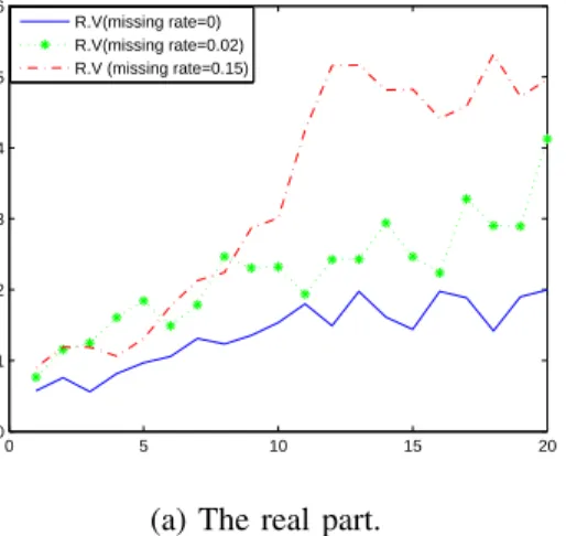
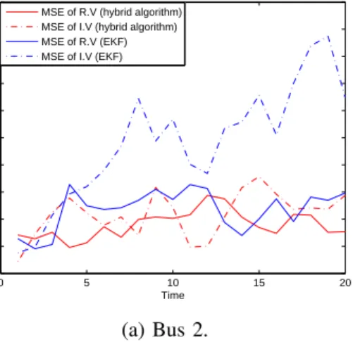
the state variables. In all the figures, “R.V” and “I.V” denote the real and imaginary part of voltage, respectively.
A. Traditional EKF vs. the Proposed EKF
In this case, the probability density function for the missing
Ξ(k) is Prob{Ξi(k) = 0} = 0.5, Prob{Ξi(k) = 1} = 0.5.
The expectation can be easily calculated as µi(k) = 0.5. The
estimated states of the representative buses2,5obtained from traditional EKF without considering the missing measurements are plotted in Fig. 1, while the counterparts obtained from the proposed EKF considering missing measurements are plotted in Fig. 2. From the comparison, it can be found that our proposed EKF algorithm performs well in the presence of missing measurements, whereas the state estimate obtained from the traditional EKF cannot track the real states when missing measurements occur randomly.
B. EKF with Individual Missing Measurements
In order to see how different missing rates impact on the estimation accuracy, three missing rates of 0.15, 0.02 and 0 (without missing measurements) are considered. The MSEs of the estimated states of buses2,5for all the three missing rates are compared in Figs. 3 and 4. The AMSE(k)in all three cases are given in the first three rows of Table II, fork= 1, . . . ,15. From the comparisons, it can be found the less the missing rate is, the more accurate the state estimation obtained from the proposed EKF algorithm will be.
C. EKF vs. Hybrid EKF and PSO Algorithm
We are now in a position to evaluate the effectiveness of including the PSO scheme in the EKF design. A comparison is made between the EKF algorithm alone and the hybrid EKF and PSO algorithm. For this purpose, the missing rate is fixed as 0.15. Regarding the penalty function parameters,θ= 1000
andh(s) =sare chosen in all the iteration steps.
For the same test system, one realization of the EKF and one realization of the hybrid algorithm are simulated simulta-neously, and the estimated states of bus voltages2,5obtained from the two algorithms are illustrated in Figs. 5 and 6. It is seen that the trajectory by the proposed hybrid approach is much closer to the true state trajectory than the one only by the EKF. TheMSE2 andMSE5 at all time instants for both
algorithms are plotted in Fig. 7. It can be found that for the same state variable, the MSE of EKF-based state estimation is bigger than the MSE of the state estimation obtained from the hybrid algorithm. Especially, when the accumulated error of EKF-based state estimation becomes bigger after several integrations, the subsequent PSO algorithm can refine the state estimation and diminish the error. The AMSEs of EKF and of the proposed hybrid algorithm are given in the last two rows of Table II. It can be found the AMSE(k) of EKF is bigger than the one of the proposed hybrid algorithm at each step.
From the comparative experiments, it can be concluded that our proposed hybrid EKF and PSO algorithm outperforms the traditional EKF algorithm in the presence of probabilistic missing measurements by including PMU measurements.
VI. CONCLUSION
In this paper, we have developed a hybrid EKF and PSO algorithm for power system dynamic state estimation. In consideration of the missing traditional measurements, a novel EKF estimator has been designed for the power system. The PMU measurements have been incorporated in the designed EKF estimator via the characterization of a set of inequality constraints. The constrained state estimation problem has been transformed to a constrained optimization problem. Then, the PSO algorithm together with the penalty function has been employed to solve the constrained optimization problem. Simulations have confirmed the effectiveness of the propose method. In our future work, we will develop our algorithms to detect the presence of contingency.
REFERENCES
[1] A. Abur and A. G. Exposito,Power system state estimation: theory and implementation. Marcel Decker, 2004.
[2] B. D. Anderson and J. B. Moore,Optimal filtering. Courier Dover Publications, 2005.
[3] T. Bi, X. Qin, and Q. Yang, “A novel hybrid state estimator for including synchronized phasor measurements,”Electric Power Systems Research, vol. 78, no. 8, pp. 1343–1352, 2008.
[4] X. Bian, X. Li, H. Chen, D. Gan, and J. Qiu, “Joint estimation of state and parameter with synchrophasorspart I: State tracking,” IEEE Transactions on Power Systems, vol. 26, no. 3, pp. 1196–1208, 2011. [5] E. Blood, B. Krogh, and M. Ilic, “Electric power system static state
estimation through Kalman filtering and load forecasting,” in Proc. Power and Energy Society General Meeting, USA, 2008, pp. 1–6. [6] M. B. Do Coutto Filho and J. de Souza, “Forecasting-aided state
estimation Part I: Panorama,” IEEE Transactions on Power Systems, vol. 24, no. 4, pp. 1667–1677, 2009.
TABLE II
THEAMSEFOR ESTIMATED STATES BY DIFFERENT ALGORITHMS WITH DIFFERENT MISSING RATES,WHEREMRDENOTES THE MISSING RATE
Time instant 1 2 3 4 5 6 7 8 9 10 11 12 13 14 15
MR= 0.00(EKF) 0.1350 0.1609 0.1748 0.2121 0.2342 0.2432 0.2366 0.2564 0.2767 0.2651 0.2707 0.2601 0.2572 0.2503 0.2751 MR= 0.02(EKF) 0.1344 0.1784 0.2091 0.2134 0.2123 0.2356 0.2550 0.2425 0.2787 0.2884 0.2851 0.3136 0.3202 0.3253 0.3578 MR= 0.15(EKF) 0.1416 0.1836 0.2152 0.2596 0.2673 0.2913 0.3341 0.3350 0.3590 0.3813 0.3858 0.4410 0.4615 0.4801 0.4612 MR= 0.15(Hybrid) 0.1342 0.1725 0.2066 0.2047 0.2226 0.2450 0.2682 0.2818 0.3135 0.2985 0.2958 0.2950 0.3050 0.3199 0.3049
Note that the results in the table are magnified103 times for clarity.
0 5 10 15 20 0 0.1 0.2 0.3 0.4 0.5 0.6 0.7 0.8 0.9 1x 10 −3 R.V(missing rate=0) R.V(missing rate=0.02) R.V (missing rate=0.15) 0 5 10 15 20 1 1.5 2 2.5 3 3.5 4 4.5 5 5.5x 10 −4 I.V(missing rate=0) I.V(missing rate=0.02) I.V (missing rate=0.15)
(a) The real part. (b) The imaginary part.
Fig. 3. The MSEs of the estimated state at bus 2 under different missing rates
0 5 10 15 20 0 1 2 3 4 5 6x 10 −4 R.V(missing rate=0) R.V(missing rate=0.02) R.V (missing rate=0.15) 0 5 10 15 20 0.5 1 1.5 2 2.5 3 3.5 4 4.5 5x 10 −4 I.V(missing rate=0) I.V(missing rate=0.02) I.V (missing rate=0.15)
(a) The real part. (b) The imaginary part.
Fig. 4. The MSEs of the estimated state at bus 5 under different missing rates
0 5 10 15 20 0.98 0.99 1 1.01 1.02 1.03 1.04 1.05 1.06 1.07 1.08 Time Voltage (p.u.) The actual R.V The estimated R.V (EKF) The estimated R.V (Hybrid algorithm)
0 5 10 15 20 0 0.01 0.02 0.03 0.04 0.05 0.06 0.07 0.08 Time Voltage (p.u.)
The actual I.V The estimated I.V (EKF) The estimated I.V (Hybrid algorithm)
(a) The real part. (b) The imaginary part.
0 5 10 15 20 0.98 0.99 1 1.01 1.02 1.03 1.04 1.05 1.06 1.07 1.08 Time Voltage (p.u.) The actual R.V The estimated R.V (EKF) The estimated R.V (Hybrid algorithm)
0 5 10 15 20 −0.04 −0.02 0 0.02 0.04 0.06 0.08 Time Voltage (p.u.)
The actual I.V The estimated I.V (EKF) The estimated I.V (Hybrid algorithm)
(a) The real part. (b) The imaginary part.
Fig. 6. The estimated state at bus 5 by EKF and the proposed hybrid algorithm
0 5 10 15 20 0 0.1 0.2 0.3 0.4 0.5 0.6 0.7 0.8 0.9 1x 10 −3 Time
Mean square error
MSE of R.V (hybrid algorithm) MSE of I.V (hybrid algorithm) MSE of R.V (EKF) MSE of I.V (EKF)
0 5 10 15 20 0 0.1 0.2 0.3 0.4 0.5 0.6 0.7 0.8 0.9 1x 10 −3 Time
Mean square error
MSE of R.V (hybrid algorithm) MSE of I.V (hybrid algorithm) MSE of R.V (EKF) MSE of I.V (EKF)
(a) Bus 2. (b) Bus 5.
Fig. 7. The MSEs of estimated states by EKF and the proposed hybrid algorithm
[7] P. Du, Z. Huang, Y. Sunet al., “Distributed dynamic state estimation with extended Kalman filter,” inProc. North American Power Sympo-sium, Singapore, 2011, pp. 1–6.
[8] R. Emami and A. Abur, “Robust measurement design by placing synchronized phasor measurements on network branches,”IEEE Trans-actions on Power Systems, vol. 25, no. 1, pp. 38–43, 2010.
[9] L. Fan, Z. Miao, and Y. Wehbe, “Application of dynamic state and parameter estimation techniques on real-world data,”IEEE Transactions on Smart Grid, vol. 4, no. 2, pp. 1133–1141, 2013.
[10] J. Hu, Z. Wang, H. Gao, and L. Stergioulas, “Extended Kalman filtering with stochastic nonlinearities and multiple missing measurements,”
Automatica, vol. 48, no. 9, pp. 2007–2015, 2012.
[11] Y. Huang, S. Werner, J. Huang, and V. Gupta, “State estimation in elec-tric power grids: Meeting new challenges presented by the requirements of the future grid,”IEEE Signal Processing Magazine, vol. 29, no. 5, pp. 33–43, 2012.
[12] J. Kennedy and R. Eberhart, “Particle swarm optimization,” in Proc. IEEE International Conference on Neural Networks, vol. 4, Hawaii, USA, 1995, pp. 1942–1948.
[13] G. N. Korres and N. M. Manousakis, “State estimation and bad data processing for systems including pmu and scada measurements,”Electric Power Systems Research, vol. 81, no. 7, pp. 1514–1524, 2011. [14] A. Simoes Costa, A. Albuquerque, and D. Bez, “An estimation fusion
method for including phasor measurements into power system real-time modeling,”IEEE Transactions on Power Systems, vol. 28, no. 2, pp. 1910–1920, 2013.
[15] D. Simon, “Kalman filtering with state constraints: a survey of linear and nonlinear algorithms,”IET Control Theory & Applications, vol. 4, no. 8, pp. 1303–1318, 2010.
[16] A. K. Singh, R. Singh, and B. C. Pal, “Stability Analysis of Networked
Control in Smart Grids,” IEEE Transactions on Smart Grid, vol 6, no. 1, pp. 381–390, 2015.
[17] X. Tai, D. Marelli, and M. Fu, “Power system dynamic state estimation with random communication packets loss,” inProc. International Sym-posium on Advanced Control of Industrial Processes, Hangzhou, China, 2011, pp. 359–362.
[18] G. Valverde and V. Terzija, “Unscented Kalman filter for power system dynamic state estimation,”IET Generation, Transmission & Distribution, vol. 5, no. 1, pp. 29–37, 2011.
[19] S. Wang, X. Meng, and T. Chen, “Wide-area control of power systems through delayed network communication,”IEEE Transactions on Con-trol Systems Technology, vol. 20, no. 2, pp. 495–503, 2012.
[20] X. Yang, X.-P. Zhang, and S. Zhou, “Coordinated algorithms for distributed state estimation with synchronized phasor measurements,”
Applied Energy, vol. 96, pp. 253–260, 2012.
[21] N. Zeng, Z. Wang, Y. Li, M. Du, and X. Liu, “A hybrid EKF and switch-ing PSO algorithm for joint state and parameter estimation of lateral flow immunoassay models,”IEEE/ACM Transactions Computational Biology and Bioinformatics, vol. 9, no. 2, pp. 321–329, 2012.
[22] M. Zhou, V. Centeno, J. Thorp, and A. Phadke, “An alternative for including phasor measurements in state estimators,”IEEE Transactions on Power Systems, vol. 21, no. 4, pp. 1930–1937, 2006.
[23] R. D. Zimmerman, C. E. Murillo-S´anchez, and R. J. Thomas, “Mat-power: Steady-state operations, planning, and analysis tools for power systems research and education,”IEEE Transactions on Power Systems, vol. 26, no. 1, pp. 12–19, 2011.