The Log-GARCH Model via ARMA Representations

Munich Personal RePEc Archive

The Log-GARCH Model via ARMA

Representations

Sucarrat, Genaro

BI Norwegian Business School

30 August 2018

Online at

https://mpra.ub.uni-muenchen.de/100386/

MPRA Paper No. 100386, posted 15 May 2020 05:17 UTC

The Log-GARCH Model via ARMA Representations

Genaro Sucarrat†

This version: 30th August 2018

[First version: 4th December 2017]

Abstract

The log-GARCH model provides a flexible framework for the modelling of economic uncertainty, financial volatility and other positively valued variables. Its exponen-tial specification ensures fitted volatilities are positive, allows for flexible dynamics, simplifies inference when parameters are equal to zero under the null, and the log-transform makes the model robust to jumps or outliers. An additional advantage is that the model admits ARMA-like representations. This means log-GARCH mod-els can readily be estimated by means of widely available software, and enables a vast range of well-known time-series results and methods. This chapter provides an overview of the log-GARCH model and its ARMA representation(s), and of how estimation can be implemented in practice. After the introduction, we delineate the univariate log-GARCH model with volatility asymmetry (“leverage”), and show how its (nonlinear) ARMA representation is obtained. Next, stationary covariates (“X”) are added, before a first-order specification with asymmetry is illustrated em-pirically. Then we turn our attention to multivariate log-GARCH-X models. We start by presenting the multivariate specification in its general form, but quickly turn our focus to specifications that can be estimated equation-by-equation – even in the presence of Dynamic Conditional Correlations (DCCs) of unknown form. Next, a multivariate non-stationary log-GARCH-X model is formulated, in which the X-covariates can be both stationary and/or nonstationary. A common critique directed towards the log-GARCH model is that its ARCH terms may not exist in the presence of inliers. An own Section is devoted to how this can be handled in prac-tice. Next, the generalisation of log-GARCH models to logarithmic Multiplicative Error Models (MEMs) is made explicit. Finally, the chapter concludes.

JEL Classification: C22, C32, C51, C58

Keywords: Financial return, volatility, ARCH, exponential GARCH, log-GARCH, Mul-tivariate GARCH

∗_{I am grateful to the Bilel, a reviewer and Hamdi Raissi for useful comments, suggestions and questions.} All errors are mine.

†_{Department of Economics, BI Norwegian Business School, Nydalsveien 37, 0484 Oslo, Norway. Email} [email protected], phone +47+46410779, fax +47+23264788. Webpage: http://www.sucarrat.net/

Contents:

1 Introduction 2

2 Univariate log-GARCH models 5

2.1 The asymmetric log-GARCH. . . 5

2.2 The ARMA representation . . . 6

2.3 Adding stationary covariates (“X”) . . . 7

2.4 Estimation of the coefficient covariance matrix . . . 7

2.5 Empirical examples . . . 9

3 Multivariate log-GARCH models 10 3.1 A multivariate asymmetric log-GARCH-X model . . . 10

3.2 Equation-by-equation estimation . . . 11

3.3 Non-stationary models . . . 12

3.4 Dynamic Conditional Correlations (DCCs) . . . 15

4 Handling zeros in practice 15

5 Modelling positively valued variables 16

6 Conclusions 17

References 17

1

Introduction

The starting point of Engle’s (1982) Autoregressive Conditional Heteroscedasticity (ARCH) class of models is

yt=µt+ǫt, ǫt=σtηt, σt>0, ηt ∼iid(0,1),

whereytdenotes the variable of interest (e.g. financial return),µtis the mean specification

(e.g. an AR-X model) or simply zero, ǫt is the error term or mean-corrected variable of

interest, σt is the conditional standard deviation or volatility, and ηt is an innovation

with mean zero and unit variance. Arguably, the most common specification of σt is the

first-order Generalised ARCH (GARCH) model of Bollerslev (1986):

σ2t =ω+α1ǫ2t−1+β1σ2t−1, ω >0, α1, β1 ≥0. (1)

Usually, this model is referred to as the GARCH(1,1) model. The log-ARCH class of models was, independently, first proposed by Geweke (1986), Pantula (1986) and Milhøj

(1987). However, the idea of modelling the log-variance goes at least back toPark(1966). The logarithmic counterpart of the GARCH(1,1) is the log-GARCH(1,1) model, which is given by

lnσ2t =ω+α1lnǫ2t−1+β1lnσt2−1, ω, α1, β1 ∈R. (2)

Just as in the GARCH model, theω is the volatility intercept,α1 is the ARCH-parameter

way), α1 controls the impact of shocks or news ηt2−1, whereas α1+β1 controls the degree

to which volatility σ2

t is persistent. If ǫt is a (mean-corrected) daily financial return,

then typical estimates of α1 and β1 lie around 0.05 and 0.9, respectively, both in the

GARCH(1,1) and log-GARCH(1,1) cases. See Section2.5 for an illustration of the latter. Let ln+x= max_{x,0_}. If P r(ηt= 0) = 0, E|lnη2t| <∞ and E(ln

+ |lnη2

t|)<∞, then a

sufficient condition for strict stationarity and ergodicity of (2) is

|α1+β1|<1, (3)

seeFrancq et al. (2013, Theorem 2.1 on p. 36).

From a user-perspective, the log-GARCH model has many attractive features:

• Fitted volatility is guaranteed to be positive due to the exponential specification. This is particularly important in higher order specifications, which may be needed in daily data with weekly periodicity (e.g. electricity prices), and in quarterly and monthly data. For example, when Engle (1982) proposed his ARCH model, he had to sub-stantially restrict his ARCH(4) specification of quarterly UK inflation uncertainty to ensure positivity of his conditional variance estimates: The specification was as-sumed to followσ2

t =ω+α1(0.4ǫ2t−1+ 0.3ǫ2t−2+ 0.2ǫ2t−3+ 0.1ǫ2t−4) so that onlyω and

α1 were estimated, see Engle (1982, p. 1002).

• No non-negativity constraints on parameters. In the GARCH model, parameters must satisfy non-negativity constraints. In the GARCH(1,1), for example, the con-straints are ω > 0 and α1, β1 ≥ 0. The first means σ2t is bounded from below and

hence cannot be smaller than ω. The second, i.e. α1, β1 ≥ 0, implies that

auto-correlations ofǫ2

t are non-negative. The log-GARCH, by contrast, does not impose

non-negativity constraints on the parameters. This means its volatility is bounded from below by 0 (and not ω as in the GARCH), and that it admits negative auto-correlations onǫ2

t. This latter is useful in regular data (e.g. daily data with a weekly

5-day or 7-day cycle, and monthly and quarterly data), since there it is likely that one or more autocorrelations of ǫ2

t are negative, see e.g. Pretis et al. (2018, Section

5.4).

• Standard inference valid under nullity of parameters. Often it is of interest to for-mulate a test in which one or more parameters are 0 under the null, say,H0: β1 = 0.

A test with this null can be carried out in a standard way (e.g. with a t-test) in the log-GARCH model, since the value of β1 lies in the interior of the admissible

parameter space under the null. In the GARCH model, by contrast, β1 = 0 lies

on the boundary of the admissible parameter space because of the non-negativity constraints. This means standard inference procedures are not valid. The practical implication of this is that it is usually easier to carry out hypothesis tests in the log-GARCH model when parameters are 0 under the null. Indeed, such tests can readily be carried out in standard software via the estimated ARMA representations.

• No non-negativity constraints on covariates. Often it is of interest to include co-variates in the σ2

t specification. For example, does a large return yesterday in a

different market (say, x2

t−1) increase volatility σt2 today? Numerous studies have

of covariates is sometimes indicated by “X”. In the log-GARCH-X model the cov-ariates are not restricted to be non-negative. In the GARCH-X model, by contrast, the covariates must be non-negative to ensure that σ2

t is positive, see e.g. Francq

and Thieu (2018). This limits the type of questions that can be answered within a GARCH-X model, and compounds the problem described above of inference un-der nullity of parameters. These restrictions and challenges do not characterise the log-GARCH.

• Invariance to power-transformations. Consider the δth. power log-GARCH(1,1) specification

lnσδt =ωδ+α1ln|ǫt−1|δ+β1lnσδt−1, δ >0. (4)

This specification is of interest if the objective is to forecast, say, the conditional standard deviation σt (or any σtδ with δ > 0) rather than σt2. In contrast to the

power GARCH counterpart, (4) can be re-written in terms of its 2nd. power as lnσt2 =ω+α1lnǫ2t−1+β1lnσ2t−1 with ω=

ωδ

δ . (5)

In other words, an estimate of (4) for any powerδ >0 is straightforwardly obtained via the estimate of (5). The power GARCH model, by contrast, is not characterised by this invariance to power transformations.

• Robustness to outliers. It is well-known that the GARCH model is fragile when out-liers or large jumps inǫtare present, see e.g.Carnero et al.(2007) and the references

therein. Similarly, the unconditional variance in Nelson’s (1991) EGARCH may not exist if ηt is too fat-tailed, e.g. student’s t, see Nelson’s own discussion in the

Ap-pendix (same place). In the log-GARCH, by contrast, the effect of η2

t is dampened

due to the log-transformation. This means the log-GARCH is much more robust to outliers or jumps and fat-tailedness of ηt. This can be illustrated by revisiting

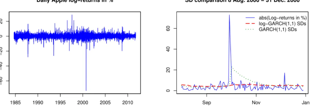
the daily Apple log-return series used by Harvey and Sucarrat (2014, pp. 320-321) to illustrate a similar robustness for the Beta-t-EGARCH model. On Thursday 28 September 2000 the firm Apple issued a profit warning after closing hours, which led its stock-value to fall from USD 26.75 to USD 12.88. Volatility, however, was not affected on the subsequent days. Figure 1contains a snapshot of the event and the surrounding days. The figure plots absolute returns, the fitted conditional standard deviations of a GARCH(1,1) specification, and the fitted conditional standard devi-ations of a log-GARCH(1,1). The GARCH forecasts (one-step-ahead) of standard deviations exceed absolute returns for almost two months after the event, a clear-cut example of forecast failure. The forecasts of the log-GARCH, by contrast, remain in the same range of variation as the absolute returns due to the log-transformation.1

This provides an empirical example of the GARCH model being prone to forecast failure in the presence of large outliers or jumps.

• Generality of specification. Two common alternatives to the log-GARCH are the Stochastic Volatility (SV) class of models, and the EGARCH of Nelson (1991). In

1_{Estimation in R (R Core Team (2018)). The GARCH model is estimated with the garch function}

from thetseriespackage of Trapletti and Hornik(2016). The log-GARCH model is estimated via its ARMA representation with thelgarchfunction from thelgarchpackage ofSucarrat(2015).

a sense, the log-GARCH is more general than these model-classes, since both admit a log-GARCH representation (but not necessarily vice-versa), seeAsai (1998), and

Francq et al. (2017).

• Log-GARCH models admit ARMA representations. This was already noted by Pan-tula(1986), and has been exploited in numerous subsequent works, see e.g. Psarada-kis and Tzavalis(1999). The usefulness of this is that a vast number of results, meth-ods and techniques from the time-series literature is available. In particular, widely available software provide routines for the estimation of ARMA and/or VARMA models can be applied, which means univariate and multivariate log-GARCH mod-els can readily be estimated in practice via their (V)ARMA representation(s). The focus of this chapter is the last of these features. In the next part, Section

2, we provide an overview of univariate models. We start by outlining an asymmetric specification, before we turn to its ARMA representation. Next we add stochastic condi-tioning covariates (“X”), and then sketch how estimates of the coefficient-covariances can be obtained in numerical software. We complete the Section by empirical illustrations of the log-GARCH(1,1) model. Section 3 provides an overview of multivariate models. Again, we start by outlining the asymmetric specification and its corresponding VARMA and VARMA-X representations. Next, we turn to specifications that are amenable to equation-by-equation estimation, both stationary and non-stationary versions, even in the presence of Dynamic Conditional Correlations (DCCs) of unknown form. The focus on multivariate specifications that can be estimated equation-by-equation is motivated by the fact estimation becomes infeasible in practice as the dimension grows too large. We end the section with a short note on how models of Dynamic Conditional Correlations (DCCs) can be estimated subsequently. Section 4 provides some suggestions on how to handle zeros in practice, whereas Section 5outlines how log-GARCH models can be used to model positively valued variables. Finally, Section6concludes and provides suggestions for further research.

2

Univariate log-GARCH models

2.1

The asymmetric log-GARCH

Financial returns are often more volatile after a fall in price compared to a rise. This is usually referred to as asymmetry or leverage. To accommodate this commonly found feature,Francq et al.(2013) proposed the asymmetric log-GARCH. If P r(ηt= 0) = 0 for

allt, then their asymmetric log-GARCH can be re-parametrised as lnσ_t2 =ω+ p X i=1 αilnǫ2t−i+ q X j=1 βjlnσ2t−j + r X k=1 γk1{ǫt−k<0}lnǫ 2 t−k, (6) where 1{ǫt<0}lnǫ 2 t = lnǫ2 t if ǫt <0 0 if ǫt <0

is the asymmetry or leverage term. The advantages of the re-parametrisation in (6) are that it is more straightforward to test for the presence of asymmetry in practice,

and that it closely resembles the most common asymmetric non-exponential GARCH-counterpart of Glosten et al. (1993). In the log-GARCH(1,1), for example, asymmetry can be tested by means of a simple t-test. The re-parametrisation implies, however, that the sufficient conditions for strict stationarity and ergodicity (i.e. Theorem 2.1 in Francq et al. (2013, p. 36)) also needs to be re-parametrised. For example, in the first order case (i.e. p=q =r = 1), the sufficient condition becomes

|α1+β1|P r(ηt>0)· |α1+β1+γ1|1−P r(ηt>0) <1.

In the absence of asymmetry we obtain the usual condition in (3), i.e. _|α1+β1|<1.

2.2

The ARMA representation

If P r(ηt = 0) = 0 and E|lnη2t| < ∞, then (6) admits, almost surely, a (nonlinear in

variables) ARMA(p, q) representation. It is obtained in two steps. First, lnη2

t is added to

each side of (6). Second, Pq_j=1βj lnηt2−E(lnηt2)

−Pqj=1βj lnηt2−E(lnηt2)

is added to the right-hand side. Re-organising gives the nonlinear ARMA representation

lnǫ2_t =ω∗+ p X i=1 φilnǫ2t−i+ q X j=1 θju2t−j+ r X k=1 γk1{ǫt−k<0}lnǫ 2 t−k+ut, ut∼iid(0, σu2), (7) where ω∗ =ω+ (1₋ q X j=1 βj)·E(lnη2t), φi =αi+βi, θj =−βj, ut = lnηt2−E(lnηt2). (8) If, in addition, E(lnη2 t)2 < _∞, then σ2 u < ∞ with σu2 = E (lnη2 t)2 −E(lnη2 t)2. Note

that the specification is a nonlinear (in variables) ARMA due to the asymmetry terms. The stationarity conditions ofFrancq et al.(2013) still apply, since lnǫ2

t is simply a sum of

the stationary variables lnσ2

t and lnηt2. The model is therefore amenable to estimation by

well-known ARMA-methods and widely available software. All the ARCH and GARCH parameters are identified via the relations in (8), and inference – even under the null of zero parameters – is readily carried out via a suitable transformation of the estimated coefficient covariance matrix, see Section2.4. However, to identify the volatility intercept

ω an estimate of E(lnη2

t) is needed, and E(lnηt2) depends on the distribution of ηt2.

Sucarrat et al. (2016) show that, under mild and general assumptions,

−ln " 1 T T X t=1 exp(ubt) # −→_p E(lnηt2), (9)

whereT is the sample size and_butis the residual from the estimated ARMA representation.

Note that the expression inside the square brackets of (9) is the smearing estimator of

Duan(1983). The motivation behind this estimator is that, if E(η2

t) = 1 and E(lnη2t)< ∞, then the population counterpart is equal to E(lnη2

t): −lnE[eut_{] =−lnE} h elnη2 t−E(lnηt2) i =₋ln 1 eE(lnη2 t) · E(η_t2) =E(lnη_t2).

Subject to suitable assumptions, therefore, consistent estimation of the ARMA representa-tion (7) and the log-momentE(lnη2

t), leads to consistent estimation of all the log-GARCH

parameters in (6).

Another notable property of the estimator in (9) is that it ensures the sample vari-ance of the standardised residuals _{η_bt} = {ǫt/σbt}, where σbt2 is the fitted value of σt2, is

approximately equal to 1 in empirical applications. This is required for _bσ2

t to be a valid

estimate of the conditional variance σ2

t. To see that the estimator in (9) ensures that the

sample variance of _{η_bt} is approximately equal to 1, let ηbt∗ = ǫt/bσ∗t denote the residual

scaled by the square root of the fitted value of the exponentiated ARMA-representation:

b

σ∗2

t = exp(lndǫ2t), where lndǫ2t is the fitted value of the ARMA-representation. Noting that

we also haveη_b∗

t = exp(but/2), it follows that b η∗ t q T−1PT t=1exp(ubt) = bη ∗ t explnT−1PT t=1exp(but)/2 = ǫt explndǫ2 t/2−Eb(lnηt2)/2 =η_bt, whereEb(lnη2

t) is the estimator in (9). In other words, the smearing estimateT−1

PT

t=1exp(but)

is approximately equal to the sample variance of_{bη∗

t}, thus ensuring the sample variance

of _{bηt} is always approximately equal to 1 in empirical applications.

2.3

Adding stationary covariates (“X”)

Letxt = (x1t, . . . , xst)′ denote a vector of strictly stationary and ergodic covariates. The

(asymmetric) log-GARCH-X model is given by lnσt2 =ω+ p X i=1 αilnǫ2t−i+ q X j=1 βjlnσt2−j + r X k=1 γk1{ǫt−k<0}lnǫ 2 t−k+ s X l=1 λlxl,t−1. (10)

A common example of a covariate is realised volatility, i.e. a volatility proxy, but another example is extended asymmetry. In other words, the extended asymmetric log-GARCH model of Francq et al.(2017) is nested in (10). The (nonlinear) ARMA-X representation is obtained in the same way as earlier (see above), and it is given by

lnǫ2t =ω∗+ p X i=1 φilnǫ2t−i+ q X j=1 θju2t−j + r X k=1 γk1{ǫt−k<0}lnǫ 2 t−k+ s X l=1 λlxl,t−1+ut, (11)

where the relations between the log-GARCH and ARMA parameters are exactly as be-fore, i.e. they are given by (8). Also, as noted earlier, no non-negativity constraints on the parameters (λ1, . . . , λs)′ nor on the covariates xt are needed. Accordingly, standard

infer-ence methods are available under the null of 0s on one or more of the λ1, . . . , λs, i.e. that

one or more covariate has no impact on volatility. To estimateE(lnη2

t), the same formula

as earlier, i.e. (9), can be used. Estimation of (10), therefore, can straightforwardly be undertaken in widely available software.

2.4

Estimation of the coefficient covariance matrix

For inference on the parameters an estimate of the coefficient covariance matrix is needed, and this expression depends on the estimator. The two most common estimators of

ARMA-models are Least Squares (LS) and Gaussian Maximum Likelihood (ML). Both provide consistent and asymptotically normal estimates under mild assumptions – even when the error ut is non-Gaussian, and most of the asymptotic properties of the two

estimators are identical, see e.g. Brockwell and Davis (2006). The LS and Gaussian ML estimators are asymptotically efficient whenηtis sufficiently fat-tailed or skewed (or both).

If, however,ηtis Gaussian, then improved efficiency can be achieved with the exponential

Chi-squared (Quasi) ML estimator proposed by Francq and Sucarrat (2018). Here, we outline the details of the LS estimator, but the approach is similar for both the Gaussian and Chi-squared ML estimators.

Let ϕ = (ω∗_{, φ}

1, . . . , φp, θ1, . . . , θq, γ1, . . . , γr, λ1, . . . , λs)′ denote the parameter of the

ARMA representation given by (11), and let

b ϕ= arg min ϕ 1 T T X t=1 u2t (12)

denote its Least Squares (LS) estimate. Often, numerical software provide utility functions for the computation of the Hessian at the optimum. Francq and Sucarrat(2017, pp. 27-28) show that this can be used to build an estimate of the coefficient covariance matrix. Specifically, they show that an estimate of the asymptotic coefficient matrix is obtained as 1 T T X t=1 b u2 t ! ·2_·Sb−1,

where ubt is the residual of the estimated ARMA-representation and Sb is the Hessian at b

ϕ based on (12). If LS estimation is implemented by minimising the sum instead of the average, i.e. b ϕ = arg min ϕ T X t=1 u2_t, (13)

then the estimate of the asymptotic coefficient matrix is modified to 1 T T X t=1 b u2t ! ·2T _·Sb−1,

whereSb is now the Hessian at ϕb based on (13).

Let ζ = (ω, α1, . . . , αp, β1, . . . , βq, γ1, . . . , γr, λ1, . . . , λs)′ denote the parameter of the

log-GARCH specification (10), and let bζ denote its estimate. An estimate of its asymp-totic coefficient matrix is available by using the relationships between the log-GARCH and ARMA-parameters given by (8). For example, ifV ard(x_b) andCovd(x,_b y_b) denote the variance of the estimatex_band the covariance of the estimates _bxand _by, respectively, then the vari-ance of the ARCH-parameterαbi is obtained asV ard(αbi) =V ard(φbi)+V ard(θbi)+2Covd(φbi,θbi).

Similarly, the variance of the GARCH-parameterβbi is obtained asV ard(βbi) = V ard(−θbi) = d

V ar(θbi). All the variances and covariances are readily available in this way, apart from

those associated with the estimate of the log-GARCH intercept ω_b. These computations are more involved and requires the use of the delta-method, see Francq and Sucarrat

2.5

Empirical examples

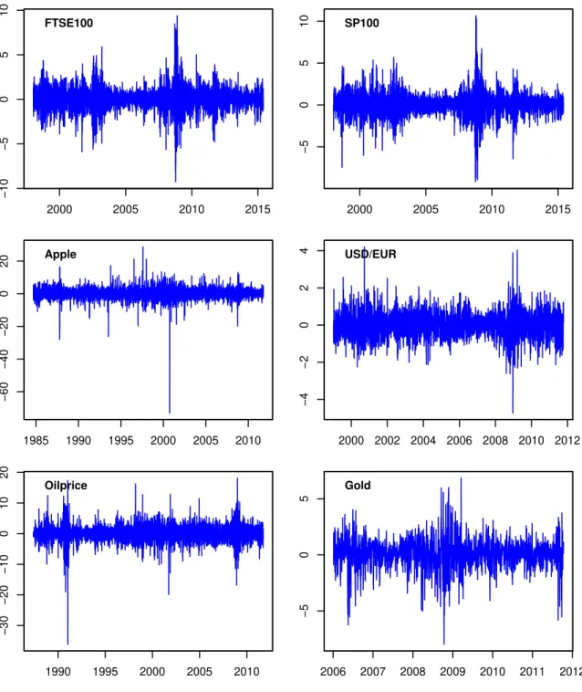
To provide an empirical illustration of the log-GARCH model, we re-visit six daily financial return series: The FTSE100 and SP100 indices (source: Bloomberg), the Apple stock price (source: Yahoo Finance, https://yahoo.finance.com), the USD/EUR exchange rate (source: The European Central Bank, http://www.ecb.int/), the brent blend oilprice (source: The US Energy Information Agency,http://www.eia.gov/) and the gold price (source: Kitco, http://www.kitco.com/). The first two return series were studied in

Francq and Sucarrat(2017, Section 5.1), whereas the latter four return series were studied in Harvey and Sucarrat (2014, Section 6). Note that the Apple series is the same as the one used to illustrate the robustness to outliers of log-GARCH models in the introduction (Section 1).

Let Pt denote the index-value or price of the asset in question in day t. The return

yt =ǫtis computed as the log-return in percent, i.e.ǫt= (lnPt−lnPt−1)·100. The sample

periods and descriptive statistics of the returns are contained in the upper part of Table

1, whereas Figure2contains graphs of the return series. As commonly found, the returns exhibit excess kurtosis relative to the normal distribution, and first-order ARCH at 5% and higher significance levels according to a Ljung and Box (1979) test for first-order autocorrelation in ǫ2

t. Also, the plots in Figure 2 confirm that volatility is persistent in

the sense that the returns are characterised by volatility clustering.

Arguably, the most common volatility model is the plain GARCH(1,1). The plain log-GARCH(1,1) counterpart is given by

lnσ2t =ω+α1lnǫt2−1+β1lnσt2−1,

and estimates of this model are contained in the middle part of Table 1. Estimation is undertaken via the ARMA(1,1) representation with the lgarch function from the R

package lgarch, see Sucarrat (2015). Usually, in ordinary GARCH(1,1) models, the estimate of the ARCH parameter α1 lies around 0.05, and the estimate of the GARCH

parameter β1 lies around 0.95. The results show that this is also the case for the

log-GARCH(1,1) models. When estimation is via the ARMA-representation, then an estimate of E(lnη2

t) is needed in order to estimate ω. If ηt ∼ N(0,1), then E(lnηt2) = −1.27. In

other words, the discrepancy from ₋1.27 can be viewed as a measure of departure from normality. For example, ifηtis a standardisedtwith 10 degrees of freedom (a “moderate”

departure from normality), then E(lnη2

t) =−1.39. The estimates ofE(lnηt2) range from −1.375 to ₋1.522, which suggests ηt is non-normal, albeit not dramatically so.

Often daily financial return series exhibit volatility asymmetry, i.e. a negative return tends to increase the volatility on the subsequent day. For stocks, this is typically referred to as a leverage effect, since leverage is often cited as the reason for the effect. For other return series, the more generic label “asymmetry” may be more appropriate, since the effect can be positive instead of negative, and since the reason for asymmetry may not be leverage. For exchange rates, for example, the presence and sign of asymmetry will usually depend on the relative strength of the two currencies in question. In other words, asymmetry is unlikely to be present in the USD/EUR exchange rate, since both the USD and Euro currencies are considered as strong currencies in international money markets. To explore the presence of volatility asymmetry in the six return series we fit a log-GARCH(1,1) model with extended asymmetry, i.e.

lnσ_t2 =ω+α1lnǫ2t−1+β1lnσt2−1+γ11{ǫt−1<0}lnǫ

2

The 1{ǫt−1<0}lnǫ

2

t−1 is the ordinary asymmetry term, and 1{ǫt−1<0} is the extended asym-metry term. As noted byFrancq et al.(2017), to ensure invariance to scale-transformations the extended asymmetry term is needed when the ordinary asymmetry term is present. If we use_±2 as critical values in a two-sidedt-test with zero as null, then both the ordinary and extended asymmetry terms are significant for the stock returns (i.e. FTSE100, SP100 and Apple). For the remaining returns, however, neither the ordinary nor the extended term is significant. In other words, the results suggest the stock returns tend to be more volatile on days subsequent to a negative return, but not the exchange rate, oilprice nor the gold return.

3

Multivariate log-GARCH models

Let yt = (y1t, . . . , yM t)′ denote an M-dimensional vector of variables (e.g. financial

re-turns) at t. A generic model of yt can be written as (see e.g. Engle (2002))

y_t = µ_t+ǫt,

ǫt = (ǫ1t, . . . , ǫM t)′, Ht=Et−1(ǫtǫ′t), D2t = diag(Ht),

η_t = D−_t1ǫt, Rt=Et−1(ηtη′t),

where µ_t is, say, a VARMA-X model, ǫt = (ǫ1t, . . . , ǫM t)′ is the error term, Ht is an

M_×M covariance matrix conditional on the past information_Ft−1, Et−1(·) is shorthand

notation for E(_·|Ft−1), D2t is a diagonal M ×M matrix with the conditional variance

or volatility σ2_t = (σ2

1t, . . . , σM t2 )′ on the diagonal, ηt= (η1t, . . . , ηM t)′ is the standardised

error, i.e. E(ηt) = 0andV ar(ηt) =1where0and1areM×1 vectors,D−t1 is a diagonal

M_×M matrix with (1/σ1t, . . . ,1/σM t)′ on the diagonal and Rt is the correlation matrix

conditional on the past. The relationships betweenHtandRtare given byHt=DtRtDt

and Rt=D−t1HtD−t1.

3.1

A multivariate asymmetric log-GARCH-X model

The multivariate asymmetric log-GARCH-X model is given by lnσ2_t =ω+ p X i=1 αilnǫ2t−i+ q X j=1 β_jlnσ2_t−j+ r X k=1 γ_k1{ǫt−k<0}lnǫ 2 t−k+λxt−1, (14) where lnσ2 t = (lnσ21t, . . . ,lnσM t2 )′, ω = (ω1, . . . , ωM)′, lnǫ2t−i = (lnǫ21,t−i, . . . ,lnǫ2M,t−i)′, 1{ǫt−k<0}lnǫ 2 t−k = (1{ǫ₁,t−k<0}lnǫ 2 1,t−k, . . . ,1{ǫM,t−k<0}lnǫ 2 M,t−k)′andxt−1 = (x1,t−1, . . . , xM,t−1)′

are allM _×1 vectors, and where

αi =    α11.i · · · α1M.i ... . .. ... αM1.i · · · αM M.i   , βj =    β11.j · · · β1M.j ... . .. ... βM1.j · · · βM M.j   , (15) γk =    γ11.k · · · γ1M.k ... . .. ... γM1.k · · · γM M.k   , λl=    λ11.l · · · λ1M.l ... . .. ... λM1.l · · · λM M.l    (16)

are all M _×M matrices. The (nonlinear) VARMA-X representation is obtained in the same way as in the univariate case, and it is given by

lnǫ2_t =ω∗+ p X i=1 φilnǫ2t−i+ q X j=1 θju2t−j+ r X k=1 γk1{ǫt−k<0}lnǫ 2 t−k+λxt−1+ut, (17) where ω∗ =ω+ I ₋ q X j=1 β_j ! E(lnη2_t), φ_i =αi+βi, θj =−βj, ut = lnηt2−E(lnη2t). (18) Without asymmetry (i.e. γ₁ = _{· · ·} = γr = 0), (17) is simply a VARMA-X model. To

conduct inference on the log-GARCH parameters, an approach similar to the one outlined in Section 2.4 can be used.

If ηt is iid, then the conditional correlation matrix Rt is constant, so that (14) is a

Constant Conditional Correlation (CCC) model. Under suitable stationarity and regu-larity conditions, the (nonlinear) VARMA-X representation (17) can then be estimated by common methods, e.g. multivariate Gaussian QML. If Rt is time-varying (and

sta-tionary), then a reasonable conjecture is that estimates will still be consistent subject to suitable assumptions. However, the asymptotic properties of such an estimator are currently unknown.

3.2

Equation-by-equation estimation

Multivariate volatility models are plagued by the “curse of dimensionality”: As the di-mension grows, estimation becomes infeasible due to the large amount of parameters that are estimated. One solution, if available, is equation-by-equation estimation. For this to be possible the GARCH-matrices (i.e.β₁, . . . ,βq) must all be diagonal, and

each ηmt, m= 1, . . . , M, must be independent of the past information Ft−1, (19)

seeFrancq and Zako¨ıan(2016). Francq and Sucarrat (2017) propose a first order version (i.e. p = q = 1) of the multivariate log-GARCH-X that satisfies these properties, and which allows for certain types of Dynamic Conditional Correlations (DCCs) of unknown form. A generalisation of their model allows for higher orders and asymmetry, and the

mth. equation in such a generalised model is given by lnσ_mt2 =ωm+ p X i=1 αm.ilnǫ2t−i+ q X j=1 βmm.jlnσm,t2 −j+ r X k=1 γm.k1{ǫt−k<0}lnǫ 2 t−k+λmxt−1, (20) whereαm.i,γm.k andλm are 1×M vectors made up of the mth. row in the matricesφi,

γ_k and λ, respectively. Theβmm.j is the mth. element of themth. column in the diagonal

matrix β_j.

The univariate ARMA-X representation of the mth. equation is lnǫ2mt = ω∗m+ p X i=1 φm.ilnǫ2t−i+ q X j=1 θmm.jum,t−j + r X k=1 γm.k1{ǫt−k<0}lnǫ 2 t−k+λmxt−1+umt, (21)

where ωm∗ =ωm+ 1− q X j=1 βmm.j

E(lnηmt2 ), φm.i =αm.i+βm.i,

θmm.j =−βmm.j and umt= lnηmt2 −E(lnηmt2 ). (22)

Under stationarity and suitable regularity conditions, (21) can be estimated consistently with standard software. Subsequently, the log-GARCH parameters can be identified via the relations in (22). To identify ωm, the formula in (9) can be applied to the residuals

of equation m to estimate E(lnη2

mt). For inference on the log-GARCH parameters in

equation m, an approach similar to the one outlined in Section 2.4 can be used. For inference that involves parameters from more than one equation, then the joint coefficient covariance is needed, see Francq and Sucarrat (2017).

For equation-by-equation estimation to be available the GARCH-matrices β₁, . . . ,β_q

must all be diagonal. To test whether this is indeed the case, a Lagrange-Multiplier (LM) test of equation m can be devised: Under the null all the elements of _{βmi.j : i 6=

m, j = 1, . . . , q_} are equal to zero, whereas under the alternative one or more elements are non-zero. Formally, this has not been pursued yet in the theoretical log-GARCH literature.

3.3

Non-stationary models

A common approach to non-stationary volatility is to decompose σ2t multiplicatively, see

(amongst other) Van Bellegem and Von Sachs (2004), Engle and Rangel (2008), Mazur and Pipien (2012), and Amado and Terasvirta (2014a, 2014b). This means

σ2_t =g_t⊙ht= (g1th1t, . . . , gM thM t)′,

whereg_tis the non-stationary component,htis the stationary component (e.g. a

GARCH-like process), and _⊙is the elementwise (Hadamard) matrix product.2 _{Escribano and} Su-carrat(2018) propose a non-stationary multivariate log-GARCH-X specification that can be estimated equation-by-equation. Their motivation was the presence of non-stochastic periodicity in the intraday electricity price market. However, their idea applies more generally. The non-stationary component in their model is given by

lngt= lng1(λf1,x f 1t), . . . ,lngM(λfM,x f M t) ′ ,

where lng1, . . . ,lngM are known functions (linear or nonlinear), xf1t, . . . ,x f

M t are known,

non-stochastic or fixed (hence the superscriptf) regressors, andλf₁, . . . ,λf_M are unknown parameters to be estimated. Neither the xfmt’s nor the lngm’s are restricted to be equal

across equations, and the lngm’s can assume a variety of shapes. In the simplest case the

lngm’s are linear functions made up of time dummies (e.g. calendar effects), but it can also

take the shape of an exponential spline as inEngle and Rangel(2008), the Fourier Flexible Form (FFF) as in Mazur and Pipien (2012), or smooth threshold models as in Amado

2_{For example, if a and b are two equally sized M ×1 vectors, say, a = (a}

1, . . . , aM)′ and b =

and Terasvirta (2014a, 2014b). The functions may also be estimated nonparametrically, as in Van Bellegem and Von Sachs(2004).

If we for notational simplicity exclude asymmetry and covariates, then the stationary component is given by lnht =ω+ p X i=1 αilneǫ2t−i+ q X j=1 β_jlnht−j, (23) where lnht = lnσ2t −lngt = (lnh1,t, . . . ,lnhM,t)′, ω = (ω1, . . . , ωM)′, lneǫ2t = (lnǫ2t −

lng_t) = (lnh1tη2₁t, . . . ,lnhM tη2M t)′, andαiandβj are bothM×M matrices as in (15). The

matrices β_j need not be diagonal. However, we will impose this restriction to enable an equation-by-equation estimation scheme. The mth. log-volatility equation thus becomes

lnσ2mt = lngmt+ lnhmt, (24) lngmt = lngm(λfm,x f mt), (25) lnhmt = ωm+ p X i=1 αm.ilneǫ2t−i+ q X j=1 βmm.jlnh2m,t−j, (26)

where αm.i is the mth. row of αi, i.e. αm.i = (αm1.i, . . . , αmM.i). Let λfm0 denote the

unconditional mean of ln_eǫ2

mt, i.e. λ f

m0 = E(lneǫ2mt) with E|lneǫ2mt| < ∞. If we add lnη2mt

to each side of (24), and thenλfm0−λ f

m0 to the right-hand side, we obtain

lnǫ2 mt=λ f m0+ lngm(λfm,x f mt) +wmt, wmt = (lneǫ2mt−λ f m0).

This is simply a regression with a fixed or non-stochastic part, i.e. λfm0+ lngm(λfm,x f mt),

and a zero-mean stationary error governed by the mean-corrected ARMA model

wmt= p X i=1 φ_m.iwt−i+ q X j=1 θmm.jum,t−j +umt, (27)

where wmt = lneǫ2mt−E(lneǫmt2 ) and wt= (w1t, . . . , wM t)′. This means the mth. equation

can be estimated in three steps: 1. Estimate λfm0 and λ

f

m via the auxiliary regression

lnǫ2mt =λ f

m0+ lngm(λfm,x f

mt) +wmt,

where λm0 is the intercept and wmt is a zero-mean stationary error-term governed

by (27). Ifλf_m enters linearly in lngm, then the parameters can simply be estimated

by OLS.

2. Fit an ARMA model to the residuals w_bmt from the first step. The relation between

the parameters of the log-GARCH model and the parameters of the mean-corrected ARMA-representation are the same as in the case where the ARMA-representation is not mean-corrected, i.e. (22). So this provides an estimate of all the log-GARCH parameters apart from the interceptωm. An estimate ofωm, however, is not needed

if the aim is to estimate σ2

first two steps provide estimates of E(lneǫ2

mt) + lngmt and Et−1(ymt), respectively.

Adding these gives

E(lneǫ2mt) + lngmt+Et−1(wmt) = lngmt+Et−1(lneǫ2mt)

= lngmt+ lnht+E(lnη2mt),

since ln_eǫ2

mt = lnhmt+ lnηmt2 . So only an estimate ofE(lnηmt2 ) is needed to complete

the estimate ofσ2 mt.

3. Estimate the log-moment E(lnη2

mt) needed to complete the estimate ofσ2mt. Again,

we can use the residuals from Step 2 in combination with (9). Summarised, then, the estimate of σ2

mt is given by b σ_mt2 = exp   bE(ln_eǫ2_mt) + ln_bgmt | {z } Step 1 +Ebt−1(wmt) | {z } Step 2 −Eb(lnη_mt2 ) | {z } Step 3  , whereEb(lneǫ2

mt) + lngbmt is the fitted value of the auxiliary regression in Step 1, Ebt−1(ymt)

is the fitted value of the mean-corrected ARMA representation in Step 2, and Eb(lnη2 mt)

is the estimate of E(lnη2

mt) in Step 3. Note that the three-step procedure can in fact be

reduced to two steps if the centred exponential Chi-squared QMLE ofFrancq and Sucarrat

(2018) is used in the second step, since E(lnη2

mt) enters explicitly as a parameter to be

estimated in the centred exponential Chi-squared density. This will also be more efficient if ηmt is normal or close to normal.

An estimate of ωm requires estimation of the other equations, in addition to equation

m. This is because the expression for E(lneǫ2

mt), which can be written as E(lneǫ2mt) =

ω∗

m +

Pp

i=1φm.iE(lneǫ 2

t), depends on the unconditional expectations of the other

equa-tions. Recalling, from (22), thatω∗

m =ωm+ 1−

Pq

j=1βmm.j

E(lnη2

mt) when the

GARCH-matrices are diagonal, solving forωm in the expression for E(lneǫ2mt) gives

ωm = (1− q X j=1 βmm.j)E(lneǫ2mt)− p X i=1 αm.iE(lneǫ2t)−(1− q X j=1 βmm.j)E(lnηmt2 ), (28)

where we have used that Pp_i=1φm.iE(lneǫ 2 t) = Pp i=1αm.iE(lneǫ2t) + Pq j=1βmm.jE(lneǫ2mt).

It should be noted that only the elements in E(lneǫ2_t), apart from the mth. entry, comes from the other equations. In other words, if there is no feedback effects (i.e. all entries in the αm.i’s apart from the mth. entry are zero), then there is no need to estimate the

other equations in order to estimateωm.

Asymmetry and stochastic covariates (“X”) can be added without affecting the estim-ation procedure just sketched. The only caveat is that they need to be mean corrected. Specifically, if xt−1 is a (r+s)×1 vector that collects all the asymmetry terms and

con-ditioning covariates of the stationary part, then they need to enter as (xt−1−x) in the

ARMA representation, where x = (x1, . . . , xM)′ are the sample means of the stationary

covariates. The stationary component is thus lnh2_t =ω+ p X i=1 αilneǫ2t−i+ q X j=1 βjlnh2t−j +δ(xt−1−x),

where δ is a parameter-matrix of appropriate size, and the mean-corrected ARMA rep-resentation of equation m is wmt= p X i=1 φm.iwt−i+ q X j=1 θmm.jum,t−j+δm(xt−1−x) +umt, (29)

wherewmt, wt and umt are defined as earlier, and δm is the mth. row ofδ. The practical

consequence of this is that the three step estimation procedure described above only requires one minor modification: Estimate (29) instead of (27) in Step 2. The other steps are unchanged, and if an estimate ofωm is needed, then formula (28) can still be used.

The asymptotic theory of non-stationary log-GARCH models has not been formally developed yet. Nevertheless, approximate inference procedures are readily available. For the stationary ARMA-representation a procedure similar to the one outlined in Section

2.4 can be used for inference within a single equation. The unknown is whether, or to what extent, this procedure is affected by the prior estimation of the non-stationary part. For inference that involves parameters from more than one equation, then an approximate joint coefficient covariance can be obtained along the lines ofFrancq and Sucarrat(2017). For inference regarding the parameters in the non-stationary part, then an approximate coefficient covariance can be computed by classical methods. For example, if the paramet-ers of the non-stationary part in equationmare estimated by OLS, and ifXmdenotes the

T_×k regressor matrix of the OLS estimator, then an approximate expression is obtained as

(X′_mXm)−1X′mΩbmXm(X′mXm)−1,

where Ωbm is an estimate of the autocovariance matrix of wm1, . . . , wmT. The estimation

results of the stationary part can be used to compute Ωbm. Indeed, if the stationary part

is an ARMA, then this procedure is already available in a number of softwares.

3.4

Dynamic Conditional Correlations (DCCs)

Assumption (19) allow for certain types of DCCs when a multivariate log-GARCH is estimated equation-by-equation. The estimation procedures described above, however, do not provide estimates of the DCCs. Nevertheless, they can – if needed – be estim-ated in a subsequent step. The estimates bσ2

1t, . . . ,bσ2M t lead to the standardised residuals b

ηt = (ηb1t, . . . ,bηM t)′, where ηbmt = ǫmt/bσmt. These residuals can be used to estimate a

DCC specification of Rt = E(ηtηt′|Ft−1). An example is the DCC of Engle (2002), or

alternatively the corrected version ofAielli (2013), see e.g. the empirical section ofFrancq and Sucarrat (2017). Another option is the robust (to spikes) DCC model proposed for electricity prices by Dupuis (2017).

4

Handling zeros in practice

Throughout we have relied on the theoretical assumption P r(ηt = 0) = 0. In practice,

however, if no conditional mean equation is fitted (i.e. we set µt = 0 for all t), we may

experience that ǫt = 0 for some t. The most straightforward solution to this is to fit a

specification µt, e.g. an intercept. This is not only justifiable in most contexts, it is also

A second solution consists of replacing zeros with some non-zero value c. One such value is a number very close to zero, say, the machine epsilon (e.g. 2.22e₋16) of the software used. This is probably the worst possible choice! The reason for this is that lnc2 _{will usually be much smaller than any empirical non-zero value of lnǫ}2

t. Accordingly,

this will induce a large ARCH shock (or inlier) at each zero location. A more sensible solution is to set c equal to a value informed by the economic application in question. If there is no (obvious) economic motivation to inform the choice of c, then one may choose a certain quantile of the non-zero values of ǫ2

t (e.g. 10%), or the sample average

of lnǫ2

t (zeros excluded), or simply the value 1. The latter is very neat and justified in

the log-GARCH(1,1) when the estimates ofα1 andβ1 are typical, i.e. about 0.05 and 0.9,

respectively. Setting c = 1 thus means lnc2 _{= 0, so that all the weight (in predicting}

lnσ2

t) is shifted on to the GARCH term, i.e. lnσ2t−1. If β1 is large (e.g. about 0.9), then

this is a very sensible solution.

A third solution consists of estimating the replacement value. This is the solution proposed by Sucarrat and Escribano (2018). Specifically, they propose to treat zeros as missing values, and to impute the missing values by the estimate of Et−1(lnǫ2t) at each

missing location. This means an optimal replacement value is inserted at each missing location in the ARMA representation, where “optimal” means the conditional (squared) forecast error is minimised, and/or that the likelihood is maximised. Arguably, treating zeros as missing values is the most appealing solution if no conditional mean is fitted. However, implementing the solution usually requires more of the user, and consistent parameter estimates are not guaranteed – in particular if the proportion of zeros is large. The freely available R package lgarch (Sucarrat (2015)) implements the missing value approach.

A fourth solution consists of adding a non-zero valuectoall the squared observations

ǫ2

1, . . . , ǫ2T. This leads to a new series {ǫt∗2} with ǫ∗t2 = ǫ2t +c and ǫ∗t = σ∗tηt∗, such that

σ∗2

t is approximately equal to σ2t +c. In other words, approximate forecasts of σ2t can

be obtained by using the estimates of σ∗2

t , and noting that σt2 ≈ σ∗t2 −c. If the values

of ǫ2

t are sufficiently large compared with c, then adding c will not alter the dynamics of

ǫ2

t in a notable manner. An example is the case where ǫ2t is interpreted as volume, i.e. a

positively valued variable (see Section5). In this caseǫ2

t will usually be much larger than,

say, c= 1.

5

Modelling positively valued variables

Engle and Russell (1998) noted that ǫ2

t could be interpreted as positively valued

vari-able, and hence showed that σ2

t can be interpreted as the conditional expectation of the

positively valued variable. Put differently, Engle and Russell (1998) showed that the ARCH-class of models can be used to model positively valued variables like duration, volume, price-spread or realised volatility. This spurred the Multiplicative Error Model (MEM) literature, seeBrownlees et al.(2012) for an overview. A particularly useful char-acteristic of the MEM interpretation is that, in practice, an ARCH estimation routine can be used to estimate a MEM. For example, suppose yt denotes the positively valued

variable in question. By providing the software in question with √y_t, then the software will return estimates of the MEM.

Formally, the MEM-class is given by

yt =ψtζt, ζt∼iid(1, σζ2), ψt, ζt ≥0,

whereψt =Et−1(yt) is interpreted as the expectation ofytconditional on past information.

Bauwens and Giot(2000) were the first to propose a logarithmic version of the MEM, i.e. a log-MEM. They noted that the MEM-interpretation associated with ordinary GARCH models was restricted by the non-negativity constraints on the parameters, and by the non-negativity constraints on the conditioning variables. Instead, they proposed a first order log-MEM with a single (stochastic) conditioning covariate. More generally, however, the univariate log-MEM(p, q) with stochastic conditioning variables can be written as

lnψt=ω+ p X i=1 αilnyt−i+ q X j=1 βjlnψt−j + s X l=1 λlxl,t−1.

That is, a univariate log-GARCH-X without asymmetry (ordinary and extended asymmetry-terms are not meaningful in MEMs). IfP r(ζt= 0) = 0 and E|lnζt|<∞, then the model

admits – as earlier – an ARMA-representation almost surely given by lnyt=ω∗+ p X i=1 φilnyt−i+ q X j=1 θjut−j+ s X l=1 λlxl,t−1+ut,

and the relations between the log-MEM and ARMA parameters are exactly the same as before, i.e. they are given by (22). The existence of an ARMA-representation of the log-MEM was, to the best of my knowledge, first pointed out byAllen et al.(2008). Similarly, the model can be extended to the multivariate case as in Section3, and non-stationarities can be introduced in the same way as in Section 3.3. Finally, fractionally integrated extensions of the log-MEM are considered in Beran et al. (2015), and in Feng and Zhou

(2015).

6

Conclusions

The log-GARCH model provides a very flexible framework for the modelling of economic uncertainty, financial volatility and a range of other positively valued variables. In this chapter we have outlined how univariate and multivariate log-GARCH models can be represented by (V)ARMA-like representations, and – as a consequence – how well-known (V)ARMA results can be used to estimate univariate and multivariate log-GARCH mod-els. Nevertheless, there is still a large, unexploited potential. There exists a wide range of well-known results on time-varying coefficients, non-stationarities, missing data and efficient estimation, amongst other, that can potentially be used to shed light on and further extend the log-GARCH class of models via its (V)ARMA-like representations.

References

Aielli, G. P. (2013). Dynamic Conditional Correlations: On Properties and Estimation.

Journal of Business and Economic Statistics 31, 282–299. http://dx.doi.org/10.

Allen, D., F. Chan, M. McAleer, and S. Peiris (2008). Finite sample properties of the QMLE for the log-acd model: Application to australian stocks. Journal of Economet-rics 147, 163–185.

Amado, C. and T. Terasvirta (2014a). Modelling Changes in the unconditional variance of long stock return series. Journal of Empirical Finance 25, 15–35.

Amado, C. and T. Terasvirta (2014b). Modelling volatility by variance decomposition.

Journal of Econometrics 175, 142–153.

Asai, M. (1998). A new method to estimate stochastic volatility models: A log-GARCH approach. Journal of the Japanese Statistical Society 28, 101–114.

Bauwens, L. and P. Giot (2000). The logarithmic ACD model: an application to the bid-ask quote process of three NYSE stocks. Annales d’Economie et de Statistique 60, 117–149.

Beran, J., Y. Feng, and S. Gosh (2015). Modelling long-range dependence and trends in duration series: an approach based on EFARIMA and ESEMIFAR models. Statistical Papers 56, 431–451.

Bollerslev, T. (1986). Generalized autoregressive conditional heteroscedasticity. Journal of Econometrics 31, 307–327.

Brockwell, P. J. and R. A. Davis (2006). Time Series: Theory and Methods. New York: Springer. 2nd. Edition, first published in 1991.

Brownlees, C., F. Cipollini, and G. Gallo (2012). Multiplicative Error Models. In L. Bauwens, C. Hafner, and S. Laurent (Eds.), Handbook of Volatility Models and Their Applications, pp. 223–247. New Jersey: Wiley.

Carnero, M. A., D. Pena, and E. Ruiz (2007). Effects of outliers on the identification and estimation of GARCH models. Journal of Time Series Analysis 28, 471–497.

Duan, N. (1983). Smearing Estimate: A Nonparametric Retransformation Method.

Journal of the Americal Statistical Association 78, pp. 605–610.

Dupuis, D. J. (2017). Electricity price dependence in new york state zones: A robust detrended correlation approach. Annals of Applied Statistics 11, 248–273.

Engle, R. (1982). Autoregressive Conditional Heteroscedasticity with Estimates of the Variance of United Kingdom Inflations. Econometrica 50, 987–1008.

Engle, R. (2002). Dynamic Conditional Correlation: A Simple Class of Multivariate Generalized Autoregressive Conditional Heteroskedasticity Models.Journal of Business and Economic Statistics 20, 339–350.

Engle, R. F. and J. G. Rangel (2008). The Spline GARCH Model for Low Frequency Volatility and its Global Macroeconomic Causes. Review of Financial Studies 21, 1187– 1222.

Engle, R. F. and J. R. Russell (1998). Autoregressive Conditional Duration: A New Model of Irregularly Spaced Transaction Data. Econometrica 66, 1127–1162.

Escribano, ´A. and G. Sucarrat (2018). Equation-by-Equation Estimation of Multivari-ate Periodic Electricity Price Volatility. Energy Economics. In press. Working paper version: MPRA Paper No. 72736 at https://mpra.ub.uni-muenchen.de/72736/. Feng, Y. and C. Zhou (2015). Forecasting financial market activity using a semiparametric

fractionally integrated Log-ACD. International Journal of Forecasting 31, 349–363. Francq, C. and G. Sucarrat (2017). An Equation-by-Equation Estimator of a Multivariate

Log-GARCH-X Model of Financial Returns. Journal of Multivariate Analysis 153, 16– 32.

Francq, C. and G. Sucarrat (2018). An Exponential Chi-Squared QMLE for Log-GARCH Models Via the ARMA Representation. Journal of Financial Econometrics 16, 129– 154. Working Paper version: http://mpra.ub.uni-muenchen.de/51783/.

Francq, C. and L. Q. Thieu (2018). Qml inference for volatility models with covariates.

Econometric Theory. https://doi.org/10.1017/S0266466617000512.

Francq, C., O. Wintenberger, and J.-M. Zako¨ıan (2013). GARCH Models Without Posit-ivity Constraints: Exponential or Log-GARCH? Journal of Econometrics 177, 34–36. Francq, C., O. Wintenberger, and J.-M. Zako¨ıan (2017). Goodness-of-fit tests for

log and exponential GARCH models. TEST. http://dx.doi.org/10.1007/

s11749-016-0506-2.

Francq, C. and J.-M. Zako¨ıan (2016). Estimating multivariate volatility models equation by equation.The Journal of the Royal Statistical Society. Series B 78, 613–635. Working paper version: MPRA Paper No. 54250: http://mpra.ub.uni-muenchen.de/54250/. Geweke, J. (1986). Modelling the Persistence of Conditional Variance: A Comment.

Econometric Reviews 5, 57–61.

Glosten, L. R., R. Jagannathan, and D. E. Runkle (1993). On the Relation between the Expected Value and the Volatility of the Nominal Excess Return on Stocks. Journal of Finance 48, 1779–1801.

Harvey, A. C. and G. Sucarrat (2014). EGARCH models with fat tails, skewness and leverage. Computational Statistics and Data Analysis 76, 320–338.

Ljung, G. and G. Box (1979). On a Measure of Lack of Fit in Time Series Models.

Biometrika 66, 265–270.

Mazur, B. and M. Pipien (2012). On the Empirical Importance of Periodicity in the Volatility of Financial Returns – Time Varying GARCH as a Second Order APC(2) Process. Central European Journal of Economic Modelling and Econometrics 4, 95–116. Milhøj, A. (1987). A Multiplicative Parametrization of ARCH Models. Research Report

Nelson, D. B. (1991). Conditional Heteroskedasticity in Asset Returns: A New Approach.

Econometrica 59, 347–370.

Pantula, S. (1986). Modelling the Persistence of Conditional Variance: A Comment.

Econometric Reviews 5, 71–73.

Park, R. (1966). Estimation with Heteroscedastic Error Terms. Econometrica 34, 888– 888.

Pretis, F., J. Reade, and G. Sucarrat (2018). Automated General-to-Specific (GETS) Re-gression Modeling and Indicator Saturation for Outliers and Structural Breaks. Journal of Statistical Software 86, 1–44.

Psaradakis, Z. and E. Tzavalis (1999). On regression-based tests for persistence in logar-ithmic volatility models. Econometric Reviews 18, 441–448.

R Core Team (2014). R: A Language and Environment for Statistical Computing. Vienna, Austria: R Foundation for Statistical Computing.

R Core Team (2018). R: A Language and Environment for Statistical Computing. Vienna, Austria: R Foundation for Statistical Computing.

Sucarrat, G. (2015).lgarch: Simulation and Estimation of Log-GARCH Models. R package version 0.6-2.

Sucarrat, G. and ´A. Escribano (2018). Estimation of Log-GARCH Models in the Presence of Zero Returns. European Journal of Finance 24, 809–827. http://dx.doi.org/10.

1080/1351847X.2017.1336452.

Sucarrat, G., S. Grønneberg, and ´A. Escribano (2016). Estimation and Inference in Univariate and Multivariate Log-GARCH-X Models When the Conditional Density is Unknown. Computational Statistics and Data Analysis 100, 582–594.

Trapletti, A. and K. Hornik (2016). tseries: Time Series Analysis and Computational Finance. R package version 0.10-35.

Van Bellegem, S. and R. Von Sachs (2004). Forecasting economic time-series with uncon-ditional time-varying variance. International Journal of Forecasting 20, 611–627.

Table 1: Empirical examples of log-GARCH models (see Section 2.5) Descriptive statistics: Sample T s2 s4 ARCH [p−val] FTSE100 5/1/1998–2/6/2015 4397 1.51 8.59 97.9 [0.00] SP100 5/1/1998–1/6/2015 4379 1.60 10.10 220.1 [0.00] Apple 10/9/1984–12/10/2011 6835 9.63 53.85 5.90 [0.02] USD/EUR 5/1/1999–12/10/2011 3274 0.45 5.45 205.9 [0.00] Oilprice 21/5/1987–4/10/2011 6190 5.59 17.47 78.6 [0.00] Gold 4/1/2006–12/10/2011 1448 1.96 6.18 6.76 [0.01]

Plain log-GARCH(1,1) models:

b ω α_b1 (s.e.) b β1 (s.e.) b E(lnη2 t) FTSE100 0.067 0.047 (0.006) (00..942008) −1.415 SP100 0.072 0.047 (0.006) (00..945008) −1.513 Apple 0.055 0.032 (0.005) (00..963007) −1.375 USD/EUR 0.025 0.022 (0.005) (00..971007) −1.380 Oilprice 0.069 0.037 (0.005) (00..952007) −1.401 Gold 0.054 0.032 (0.007) (00..958010) −1.522

Asymmetric log-GARCH(1,1) models:

b ω α_b1 (s.e.) b β1 (s.e.) b γ1 (s.e.) b λ1 (s.e.) b E(lnηt2) FTSE100 −0.126 0.003 (0.006) (00..945006) (00..069010) (00..362035) −1.365 SP100 −0.112 0.011 (0.007) (00..934008) (00..070012) (00..374040) −1.453 Apple 0.046 0.028 (0.007) (00..954009) (00..016007) (00..053019) −1.361 USD/EUR 0.013 0.024 (0.007) (00..970007) −(00..010)003 (00..021027) −1.374 Oilprice 0.058 0.030 (0.006) (00..952007) (00..014008) (00..024016) −1.396 Gold 0.063 0.036 (0.009) (00..961011) −(00..014)012 −(00.049).025 −1.517

T, number of non-missing returns. s2, sample variance. s4, sample kurtosis. ARCH,Ljung and Box(1979) test statistic of first-order serial correlation in the squared return. p−val, thep-value of the test-statistic. s.e., approximate standard errors (obtained via the numerically estimated Hessian) of estimate. All computations inR (R Core Team(2014)), estimation with thelgarch

1985 1990 1995 2000 2005 2010 −60 −40 −20 0 20

Daily Apple log−returns in %

Sep Nov Jan

0

20

40

60

SD comparison 8 Aug. 2000 − 31 Dec. 2000

abs(Log−returns in %) log−GARCH(1,1) SDs GARCH(1,1) SDs

Figure 1: Daily Apple log-return in % (left graph) and a snapshot (right graph) of the period before and after a profit warning 28 September 2000, see Section 1. Datasource: Yahoo Finance

2000 2005 2010 2015 −10 −5 0 5 10 FTSE100 2000 2005 2010 2015 −5 0 5 10 SP100 1985 1990 1995 2000 2005 2010 −60 −40 −20 0 20 Apple 2000 2002 2004 2006 2008 2010 2012 −4 −2 0 2 4 _USD/EUR 1990 1995 2000 2005 2010 −30 −20 −10 0 10 20 Oilprice 2006 2007 2008 2009 2010 2011 2012 −5 0 5 Gold

Figure 2: Daily financial log-returns in %, see Section 2.5 and Table 1. Datasources: Bloomberg, Yahoo Finance, European Central Bank, US Energy Information Agency and Kitco