Arnab Rahman Chowdhury
Distributed deep learning inference in
fog networks
Master’s Thesis Espoo, July 30, 2020
Supervisors: Professor Mario Di Francesco, Aalto University
Professor Frank Alexander Kraemer, Norwegian University of Science and Technology
Master’s Programme in Security and Cloud Computing MASTER’S THESIS Author: Arnab Rahman Chowdhury
Title:
Distributed deep learning inference in fog networks
Date: July 30, 2020 Pages: 82
Major: Security and Cloud Computing Code: SCI3084 Supervisors: Professor Mario Di Francesco
Professor Frank Alexander Kraemer Advisor: Thaha Mohammed M.Sc. (Tech.)
Today’s smart devices are equipped with powerful integrated chips and built-in heterogeneous sensors that can leverage their potential to execute heavy compu-tation and produce a large amount of sensor data. For instance, modern smart cameras integrate artificial intelligence to capture images that detect any objects in the scene and change parameters, such as contrast and color based on envi-ronmental conditions. The accuracy of the object recognition and classification achieved by intelligent applications has improved due to recent advancements in artificial intelligence (AI) and machine learning (ML), particularly, deep neural networks (DNNs).
Despite the capability to carry out some AI/ML computation, smart devices have limited battery power and computing resources. Therefore, DNN computation is generally offloaded to powerful computing nodes such as cloud servers. However, it is challenging to satisfy latency, reliability, and bandwidth constraints in cloud-based AI. Thus, in recent years, AI services and tasks have been pushed closer to the end-users by taking advantage of the fog computing paradigm to meet these requirements. Generally, the trained DNN models are offloaded to the fog devices for DNN inference. This is accomplished by partitioning the DNN and distributing the computation in fog networks.
This thesis addresses offloading DNN inference by dividing and distributing a pre-trained network onto heterogeneous embedded devices. Specifically, it im-plements the adaptive partitioning and offloading algorithm based on matching theory proposed in an article by Mohammed et al. [25]. The implementation was evaluated in a fog testbed, including Nvidia Jetson nano devices. The obtained results show that the adaptive solution outperforms other schemes (Random and Greedy) with respect to computation time and communication latency.
Keywords: DNN inference, task partitioning, task offloading, distributed algorithm, DNN frameworks and architectures
Language: English
I would like to thank my thesis supervisors, Mario Di Francesco, Frank Alexander Kraemer, and my advisor Thaha Mohammed for helping and guid-ing me throughout the thesis process.
I am grateful to my friends for giving me moral support to complete the thesis on time.
Finally, I must express my gratitude to my parents for encouraging me to stay strong during the pandemic situation as they reside 4000 kilometers away from me. This accomplishment would not have been possible without them.
Thank you.
Espoo, July 30, 2020
Arnab Rahman Chowdhury
DNN Deep Neural Network AI Artificial Intelligence
ML Machine Learning
RBM Restricted Boltzmann Machine DBN Deep Belief Network
GAN Generative Adversarial Network RNN Recurrent/Recursive Neural Network LSTM Long Short Term Memory
GRU Gated Recurrent Unit
CNN Convolutional Neural Network NiN Network in Network
ReLU Rectified Linear Unit
DDNN Distributed Deep Neural Network DINA Distributed INference Acceleration
DINA-P Distributed INference Acceleration-Partitioning DINA-O Distributed INference Acceleration-Offloading gRPC gRPC Remote Procedure Call
MQTT Message Queuing Telemetry Transport BDD100k Berkeley Deep Drive dataset
Abbreviations and Acronyms 4
1 Introduction 7
1.1 Problem statement . . . 8
1.2 Structure of the thesis . . . 9
2 Deep neural networks (DNNs) 10 2.1 Overview . . . 10
2.2 DNN architectures . . . 12
2.3 Unsupervised Pretrained Networks (UPNs) . . . 15
2.3.1 Restricted Boltzmann Machines (RBMs) . . . 15
2.3.2 Autoencoders . . . 16
2.3.3 Deep Belief Networks (DBNs) . . . 16
2.3.4 Generative Adversarial Networks (GANs) . . . 17
2.4 Convolutional Neural Networks (CNNs) . . . 18
2.4.1 AlexNet . . . 23
2.4.2 VGG . . . 24
2.4.3 ResNet . . . 26
2.4.4 Network-in-Network . . . 28
2.5 Recurrent Neural Networks (RNNs) . . . 28
2.5.1 Long Short Term Memory (LSTM) . . . 30
2.5.2 Gated Recurrent Units (GRUs) . . . 31
2.6 Recursive Neural Networks (RNNs) . . . 33
3 Distributed DNN inference 35 3.1 Distributed mobile computing system . . . 35
3.2 Neurosurgeon . . . 36
3.3 DNN Surgery . . . 38
3.4 Distributed deep neural network . . . 40
3.5 Distributed inference acceleration (DINA) . . . 41
3.5.1 Fine-grained adaptive partitioning (DINA-P) . . . 43 5
4 Implementation 50
4.1 Frameworks, libraries and tools . . . 50
4.2 Implementation details . . . 52
4.2.1 Training models . . . 52
4.2.2 Implementing DINA-P and DINA-O . . . 54
4.2.3 Implementation approach . . . 55
5 Evaluation 57 5.1 Experimental setup . . . 57
5.2 Selection of the dataset . . . 58
5.3 Network topology . . . 59
5.4 Experimental results . . . 60
6 Conclusion 64 A Communication protocols 70 A.1 Message Queuing Telemetry Transport . . . 70
A.1.1 Protocol operations . . . 70
A.1.2 Evaluation . . . 73
A.2 gRPC Remote Procedure Calls . . . 74
A.2.1 Protocol operations . . . 75
A.2.2 Evaluation . . . 76
A.3 Protocols comparison . . . 77
B Time comparison 78
Introduction
In recent years, the development of high-performance computing is steadily increasing. In particular, the computing capability of modern computers and embedded devices has increased due to the improvement of central process-ing unit and graphics processprocess-ing unit architectures. As a result, these devices are capable of computing complex functions of artificial intelligence (AI) and machine learning (ML) for different applications, such as image and natu-ral language processing, speech recognition, augmented reality, and cogni-tive assistance. Moreover, embedded devices equipped with sensors for data collection are mostly targeted for applications leveraging machine learning. According to Cisco, the number of smart devices connected via the inter-net will grow more than 12 billion by 2022 [5]. Therefore, the scope of data generation will increase for machine learning-based applications. In addition, the availability and the maintenance cost of cloud infrastructures have de-creased in recent times, inspiring AI/ML-based applications to execute heavy computation in the cloud.
Generally, most of the machine learning applications are computed at smart devices, and sometimes the heavy computations are offloaded to the cloud. Smart devices are unable to execute heavy computation of AI/ML-based applications due to a lack of computing power and limited resources. Instead, they offload the computation to the cloud or employ a simple ma-chine learning model, such as Support Vector Mama-chines. However, offloading computation to the cloud adds extra costs due to communication: a high response time and a low throughput; moreover, the simpler machine learning models provide results with reduced accuracy. Fog computing has emerged to address these problems. In fact, fog computing provides decentralized com-puting infrastructure that brings the benefits and comcom-puting power of the cloud closer to the source of data [1].
Deep Neural Networks (DNNs) have recently been used in a variety of 7
intelligent applications. DNNs require heavy computing power and resources, significantly increase the computation burden at the end devices. Moreover, DNNs are progressing towards deeper structures to provide more system accuracy and precision [14, 32, 36]. Researches in deep neural networks have proposed different techniques that involve partitioning and offloading the DNN structure (model) into a distributed computing hierarchy [16, 18, 23, 38]. A distributed computing hierarchy consists of the local network, the fog, and the cloud. This process distributes the computation costs and parallelizes the computation to adopt scalability and efficiency.
1.1
Problem statement
Despite their growth, AI/ML-based applications encounter important key challenges. Smart (embedded) devices have lower energy and computing re-sources, whereas intelligent applications (e.g., image recognition, natural lan-guage processing, and speech detection) require high processing power. More-over, some of these applications are latency-sensitive and safety-critical, such as augmented reality and cooperative autonomous driving. Dynamic network conditions also affect collaborative partitioning and distribution of compu-tation [16, 18]. Considering the challenges, this thesis aims to answer the following questions:
• Which approach is appropriate to address the challenges imposed by AI/ML-based applications?
• Are solutions for addressing the challenges proposed in the literature practical for use at resource-constrained embedded devices?
This thesis addresses offloading DNN inference by dividing and distributing a pre-trained network onto heterogeneous embedded devices. In particular, it implements an adaptive partitioning and a distributed offloading algo-rithms based on matching theory introduced in the work by Mohammed et al. [25]. DNN inference refers to the technique of predicting the results of a DNN process while encountering new data. The implementation was evalu-ated in a testbed consists of heterogeneous fog devices (Nvidia Jetson Nano devices).
The main contributions of this thesis are as follows. First, it implements an adaptive partitioning scheme based on the computing capability and the utilities of the fog nodes. Utility is used to express association preference among the end devices and the fog nodes. The source DNN is divided into sublayers by the adaptive partitioning algorithm in order to offload to fog
networks. Finally, experiments are carried out by considering three different schemes: Adaptive, Random, and Greedy. The obtained results based on a large dataset and four state-of-the-art DNN architectures demonstrate that the adaptive solution outperforms other schemes (Random and Greedy) in terms of computation time and communication latency.
1.2
Structure of the thesis
The rest of the thesis is organized as follows. Chapter 2 overviews artificial intelligence and machine learning, then presents different DNN architectures in some detail. Chapter 3 discusses the most important research targeting DNN inference acceleration. Chapter 4 details the implementation of the offloading framework based on matching theory proposed by Mohammed et al. [25]. Chapter 5 evaluates the related adaptive partitioning approach against the other two strategies, namely, random partitioning and greedy offloading. Finally, Chapter 6 concludes the thesis and describes possible future research.
Deep neural networks (DNNs)
A deep neural network (DNN) is a member of a broad family in artificial intelligence; especially, it is considered a sub-field of machine learning. It is a computational model inspired by the biological structure of the brain cells, which consists of interconnected nodes (neurons) that can learn from experi-ence by modifying their connections and parameters. DNN is massively used in different application areas, such as speech recognition, natural language processing, computer vision, image, and video surveillance. With the help of DNN, AI can be trained by using supervised and unsupervised learning data and predict results.The rest of this chapter describes the overview, the DNN architectural components, and the categories of DNN architectures in general.
2.1
Overview
Since an early age, computer scientists have been deriving their thoughts to design and build such a machine that would act identical to humans. Alan Turing, the father of theoretical computer science, developed a Turing test, which could evaluate the intelligent behavior of a machine in comparison to humans. In 1956, for the first time, the term Artificial Intelligence (AI) was introduced by John McCarthy.
Artificial intelligence refers to such a computer system that can perceive and learn knowledge, make reasoning and decisions based on the acquired knowledge, and act accordingly in an uncertain and complicated environ-ment. There are two categories of AI in the modern era: the Narrow AI/Weak AI and the General AI/Strong AI. The narrow AI has the ability to handle only one sophisticated task. In contrast, several narrow AI can be combined to achieve a wide range of goals in the general AI. For example, in a
contrast, if the system can detect an object with the best accuracy, process voice commands and adopt in any complicated situations at the same time indicates as general AI.
The first intelligent machine-building approach is known as symbolic AI. This approach works manually based on human-readable symbols and a set of rules for manipulating the symbols. A symbol may represent in a character string to describe the task in words. For example, a symbolic representation of a “Wooden chair” is given in Figure 2.1, inspired by [24].
Wooden Chair
Origin Structure Kind
Furniture shop Frame Furniture
Material Color Shape
Wood Metal Screw Dining chair
Figure 2.1: The symbolic representation of a wooden chair.
The manual input process of symbolic AI system is inappropriate for handling real-life problems. It also imposes a significant challenge to declare all the symbols and the rules to fit with real-world applications. To alle-viate the problems, researches apply machine learning approach. Machine Learning (ML) is a statistical method that provides the system ability to learn directly from the data and improve from experience without human intervention. As the example mentioned earlier in the symbolic approach, if different categories of chair images are fed into the machine learning al-gorithm, the algorithm will be able to detect the chair and its category by learning features, such as edges, patterns, and textures.
Supervised learning: In supervised learning, the training input data and the target output are known. The supervised learning algorithm learns from the input data by comparing the generated prediction result with the target output. It is an iterative learning process and achieves an acceptable level of performance after a certain iterations. Linear regression, Random forest, and Support vector are some popular supervised learning algorithms. Unsupervised learning: In unsupervised learning, only the training data is available. The unsupervised learning algorithm learns by discovering the features of the input data and accumulates the learning into its knowledge domain. This method generates new input data based on the observation of the same set of data. K-means and Apriori are some practiced unsupervised learning algorithms.
With the advancement of computing capabilities and big data technolo-gies, machine learning introduces a system architecture known as Artificial Neural Network (ANN). ANN was introduced in the late ’40s, requiring a high computational power and access to a large dataset. In recent times, the powerful CPU and GPU, and the cloud infrastructures revive the ANN technology to take care of the complex AI tasks proficiently. A deep neural network is one of the kinds of artificial neural networks.
2.2
DNN architectures
The architectural components of a neural network are layers, parameters, hy-perparameters, activation functions, loss functions, and optimization meth-ods. The layers are constructed by neurons, which are known as units [29]. Units are a symbolic representation of biological neurons. Figure 2.2 illus-trates a basic structure of a neural network.
Layers: A layer represents a collection of units that operates together at a specific depth of the neural network. There are two types of layers in a neural network, such as the input layer and the hidden layers. The output layer is categorized under the hidden layers. The input layer represents the input features that go through the units of hidden layers to generate prediction in the output layer. The hidden layers learn different aspects of the input data by breaking it down into different levels of abstraction. To understand the hidden layer’s concept, let us consider an image recognition example of a four-wheel vehicle. In abstract terms, the first hidden layer is responsible for identifying pixels of light and dark, and the second hidden layer detects edges and simple shapes. Primarily, the hidden layers at the beginning of the DNN identify simple structural components, but the deeper hidden layers detect more complex structure of the image.
x2 w2
Σ
f
Activate function y Output x1 w1 • • • xn wn Weights InputsFigure 2.2: A basic structure of a neural network.
Parameters: Parameters in neural networks are configuration variables. They are subjective to the model and may vary based on different neural network architecture. The weights and the biases are such parameters which are used to form the network connection.
Hyperparameters: Hyperparameters are used to tune the neural net-work and configure settings to achieve effective performance. The size of the layer, learning rate, dropout, mini-batch size, number of epochs, and nor-malization of input data are included in the hyperparameters.
• Layer size: The layer size defines the number of units in a layer.
• Learning rate: The learning rate governs how much to adjust in the model based on the estimated error calculated during model training. A high learning rate may cause the convergence to sub-optimal solu-tions, whereas a low learning rate takes a more prolonged period for the training process to complete.
• Dropout: The dropout mechanism discards units from the hidden layers to improve the neural network training and to overcome the over-fitting problem. The over-fitting problem occurs when the trained model works efficiently with the training data (seen data) but works poorly with the testing data (unseen data).
• Mini-batch size: The mini-batch size refers to how many samples will propagate through the network at a time. The network trains faster with mini-batches as the model parameters are updated after each propagation. For example, let us assume the total sample size is
1280, and the mini-batch size is 128. The model parameters will be updated 10×for each propagation.
• Number of epochs: The number of epochs defines the number of times the complete data set propagates through the learning algorithm.
• Normalization: In vector representation of the input data, the data are scaled to a specified range, such as [0,1], [-1,1], which affects the activation in the neural network.
Activation functions:An activation function is used to restrict the out-put of a layer to a specific limit and add non-linearity in the neural network. The activation function helps the network to learn the complex pattern in the data set. Some commonly used activation functions are sigmoid, tanh and Rectified Linear Unit (ReLU).
Loss functions: Loss functions assess the compliance between the pre-dicted output and the supervised learning output. The loss functions deter-mine the misclassification cost. Based on the calculated loss, model param-eters are updated accordingly through the backward propagation method. Some commonly used loss functions are Mean Squared Error (Regression problem) and Cross-Entropy Loss (binary and multi-class classification problem).
Optimization methods: Optimization methods help to minimize loss functions by updating the parameter values through optimization algorithms. These methods aim to find the best set of parameter values, in other words, a trained model that gives minimal loss. The optimization algorithms are categorized into two types, such as first-order optimization algorithms (e.g., Gradient Descent, Stochastic Gradient Descent) and second-order op-timization algorithms (e.g.,Newton method,Conjugate Gradient). The most widely used first-order optimization algorithm is Adam, which computes the adaptive learning rate for each parameter [19].
A historical evolution of DNN architectures is shown in Figure 2.3. Ac-cording to Patterson et al. [29], there are four major DNN architectures in practice.
1. Unsupervised Pretrained Networks (UPNs) 2. Convolutional Neural Networks (CNNs) 3. Recurrent Neural Networks (RNNs) 4. Recursive Neural Networks (RNNs)
RNN LSTM CNN
DBN GRU
Figure 2.3: The Evolution of DNN architectures.
2.3
Unsupervised Pretrained Networks (UPNs)
Unsupervised pretraining helps to extract features from an unlabeled data set. There are many architectures used for unsupervised pretraining, and the followings are the most popular neural networks.
1. Restricted Boltzmann Machines (RBMs) 2. Autoencoders
3. Deep Belief Networks (DBNs)
4. Generative Adversarial Networks (GANs)
2.3.1
Restricted Boltzmann Machines (RBMs)
Restricted Boltzmann Machines (RBMs) are two-layered neural networks widely used for dimensionality reduction (feature selection and extraction), classification, regression, collaborative filtering, and topic modeling. They can learn a probability distribution over its input dataset. A fully bipartite graph connects both layers (visible and hidden layer) of RBMs. Units of the same layer are not connected, that makes them restricted and different from Boltzmann Machine.
In RBMs, there are two additional bias layers (visible bias and hidden bias), which makes it different than Autoencoders. The hidden and the visi-ble bias layers are used in the forward pass and reconstruction phase, respec-tively. Figure 2.4 illustrates the forward pass and the reconstruction phase of RBMs. The RBMs construct error by subtracting the inputs from the recon-structed inputs and tune the model parameters (e.g., weights) accordingly. Due to the behavior of the RBMs, they are known as generative models as they generate new samples of data from the same distribution.
+ bias + bias f f In p u ts
Visible Hidden Activation Output Function bias + bias + f f In p u ts
Visible Hidden Output Activation
Function
bias +
f
Forward Pass Inputs Reconstruction
Figure 2.4: RBMs forward pass and reconstruction phase.
2.3.2
Autoencoders
Autoencoders are used to learn an efficient way of compressing and encoding data to construct new data, closer to the original input. They reduce data dimensions by ignoring noise in the data. Autoencoders are constructed by four significant parts: encoder, bottleneck (hidden layers), decoder, and re-construction loss. Figure 2.5 shows a basic structure of autoencoders. The bottlenecks are the autoencoders’ key feature, which constrains a compressed knowledge representation of the input.
Autoencoders are almost similar to multi-layer perceptron with some dif-ferences. One of the differences is that both the input and the output layers of autoencoders have the same number of units. Autoencoders use unla-beled data in unsupervised learning and build a compressed representation of inputs with bottlenecks. Variational autoencoders, sparse autoencoders, denoising autoencoders, and contractive autoencoders are some autoencoder variants widely used in practice. The application areas of autoencoders are anomaly detection and image denoising.
2.3.3
Deep Belief Networks (DBNs)
Deep Belief Networks (DBNs) are probabilistic unsupervised learning algo-rithms. They are constructed by the stack of Restricted Boltzmann Machines (RBMs), consisting of multiple hidden and visible layers of stochastic and la-tent variables. Unlike other models, each layer of DBNs knows the entire input data. The process through which DBNs learn is a greedy approach. In a greedy learning algorithm, the optimal choice is made at each step of the process, which leads to the global optimum. Figure 2.6 shows a basic architecture of DBNs.
Figure 2.5: A basic structure of autoencoders.
The DBN’s overall process can be categorized into two phases, such as the pre-train phase and the fine-tuning phase. Learning features in an unsuper-vised fashion is considered as the pre-train phase. The RBMs learn higher-level features from the distribution of data through each layer progressively, which eventually use the learned features as input to the higher level. When the learned features are used as initial model parameters in a feed-forward network; this phase is called the fine-tuning phase. In the feed-forward net-works, backpropagation is the key for tuning the model parameters. Normal backpropagation is used with a low learning rate to find the best value for model parameters.
2.3.4
Generative Adversarial Networks (GANs)
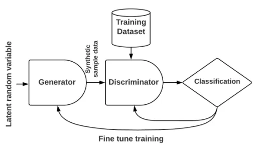
Generative Adversarial Networks (GANs) [9] are a combination of generative and discriminative learning algorithms. The generative algorithm tries to generate sample inputs for the discriminative algorithm to classify whether the data is populated from the generator or the training data set. GANs are used to build efficient classifiers by generating sample images and videos. Moreover, they are also used to create fake media content, such as Deepfakes. Figure 2.7 illustrates a visual overview of the GANs architecture.
The GANs are formed by two neural networks, such as a generator and a discriminator, and simultaneously train two models. The generator pro-duces synthetic sample data from a random noise and trains the model to provide more realistic sample data, which are fed through the
discrimina-Figure 2.6: A basic architecture of DBNs.
tor to determine whether the data is real or synthetic. The discriminators are usually standard Convolutional Neural Networks (CNNs). The genera-tors use deconvolutional networks to generate synthetic sample images. The gradient of the output of discriminators helps the generator to produce more realistic data by making small changes. In both networks, backpropagation is used to train the model efficiently. GAN is considered a recursive process of generating more realistic data and a useful classifier that can detect the difference between synthetic and training data.
2.4
Convolutional Neural Networks (CNNs)
Convolutional Neural Network (CNN), also known as ConvNet, is a class of neural networks where a linear convolution operates instead of matrix mul-tiplication in network layers. This architecture has taken inspiration from biological processes, especially the connectivity pattern of the visual cortex neurons. Some regions of visual cortex cells trigger to a specific pattern of
Figure 2.7: A visual overview of GANs architecture.
visual fields such as edges, color, and curves. All the sensitive neurons are organized in a columnar fashion to produce visual perception and try to lo-cate specific characteristics of the observed object [17]. The basic progression of the CNN is similar to the visual cortex working process. The CNN learns higher-order features of data through convolution operation. First, it starts by classifying the lower-level features, and more sophisticated features are analyzed as the network progresses. Such architecture is useful for object recognition in images and videos, translating natural language and senti-ments.
The goal of CNN is to transform input data starting from the input layer through intermediate connected layers into a set of classes. The output layer shows the difference of the input images. The high-level overview of the CNN architecture is as follows.
• Input layer
• Learning layer (feature extraction)
The learning layer or the feature extraction layer executes a repetitive pattern of sequence:
• Convolution layer (linear operation)
• Activation function (e.g. ReLU,sigmoid, tanh)
• Pooling layer
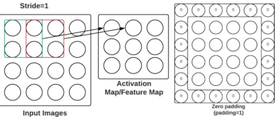
The first layer in the CNN is always a convolutional layer. The input is a tensor of shape [number of images/batch] × [width of image] × [height of image]×[depth of image (channels)]. A feature identifier, known as a filter/a kernel, convolves over the receptive field from left to right through the input images to extract lower-level features and generate an activation map or a feature map. The receptive field refers to a region in the input data that stimulates when the filter/the kernel is applied to extract features, and the feature map represents the result of the extraction. The depth of the kernel must be kept the same as the depth of input. A visual illustration is given in Figure 2.8. In the series of the feature-extraction layers, the output of one convolutional layer interprets as the input to the next convolutional layer. As it progresses, more complex features are extracted. Zeiler et al. [40] represents a visualization of intermediate features and the classifier’s operation in a CNN. The following formula provides the output size of a given convolutional layer. Here, W = input volume size, K = kernel size, P = padding and S = stride.
output= W −K −2P
S + 1
During the design consideration of CNN, some of the hyperparameters need to be considered, such as the filter/kernel size, the stride, and the padding. The stride represents the number of shifts while the kernel is slid-ing through the input images. It controls the slidslid-ing movement of the kernel over input volume. The spatial dimension decreases as the convolution op-eration progresses. Zero padding is added to the image’s border to preserve more information of the original input volume to detect lower-level features. The choice of an appropriate hyperparameter largely depends on the type of training dataset. Figure 2.9 visualizes the stride and the padding of the convolution layer.
After each convolution layer, the activation function is applied to in-troduce non-linearity. In recent years, the Rectified Linear Unit (ReLU) becomes very popular due to its faster training efficiency and capability to alleviate the vanishing gradient decent problem. The vanishing gradient prob-lem occurs during propagation phase of network training. In the back-propagation algorithm, the gradient is calculated based on the loss function
Figure 2.8: A visual illustration of CNN convolution operation.
Figure 2.9: A visual illustration of stride and padding in CNN convolution operation.
and it becomes infinitely smaller in a deep network. Thus, the performance gets saturated and degrades rapidly. The ReLU also improves the perfor-mance of neural network [26]. It applies the function f(x) = max(0, x) to all the values of the convolution layer output. Some other non-linear acti-vation functions, such as sigmoid (σ(x) = 1/(1−e−x)), tanh (tanh(x) =
(ex−e−x)/(ex+e−x)) are popular as well in neural network.
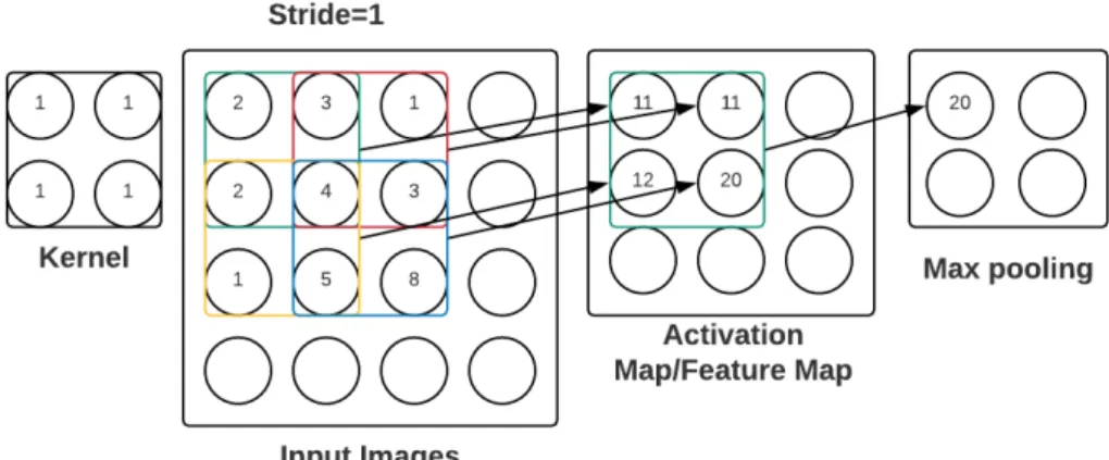
Depending on the structure and the type of dataset, after the activa-tion layer, the pooling layer is applied. It is also known as non-linear down-sampling. The purpose of pooling layer is two-fold. First, reducing the
compu-tation cost by compressing the number of model parameters, such as weights and second, controlling overfitting problem. In the overfitting problem, the model is trained in such a way that it learns the details and the noise of the training data, which impacts negatively on the performance of the model on new data. There are different options for pooling to choose, such as max pooling, average pooling, L2-norm pooling. Figure 2.10 shows how max-pooling works in convolution neural network. Dropout [35] is another way to reduce overfitting. Units of CNN layers deactivate randomly in dropout phase. Dropout is applied mostly in fully connected layers of CNNs.
Figure 2.10: Example of max-pooling in CNN.
After several convolutional and pooling layers, the network introduces fully-connected layers to co-relate the higher-level features to a particular class, which provides the outcome of the network. Fully-connected layers take the output of the last convolutional or the pooling layer as input and output N-dimensional vectors. N-dimensional vector represents the number of classes/categories that can be identified from the data. Figure 2.11 illus-trates a complete overview of CNN.
Many state-of-the-art convolutional neural networks are introduced by AI researchers, which can classify and predict objects from a set of images and video streaming. For DNN inference, data are trained by different image classification architectures, such as AlexNet [20], ResNet [14], VGG [32], and NiN [22] in this thesis. These architectures are also used for predictions and classifications. This section will briefly explain the benchmark CNNs for object recognition and image classification tasks.
Figure 2.11: A complete overview of convolutional neural network.
2.4.1
AlexNet
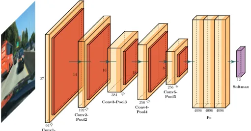
One of the most notable publications in the field of computer vision is “Ima-geNet Classification with Deep Convolutional Networks” [20]. Authors have proposed a deep convolutional neural network that can classify images with the top-5 test error rate of 15.3%. AlexNet can classify images in 1,000 classes. AlexNet has eight learned layers composed of five convolutional layers and three fully-connected layers.
• The first convolutional layer takes 224 × 224 × 3 as input where 224 represents the dimension of the image, and three represents the channel (e.g., RGB). The input is filtered with 96 kernels of size 11 × 11 × 3 with a stride of 4 pixels. The following convolutional layer filters the output of the former convolutional layer. The second convolutional layer filters with 256 kernels of size 5 × 5 ×48.
• The last three convolutional layers do not have any pooling or normal-ization layers in between and are connected.
• The third, fourth, and the last convolutional layers filters with 384 kernels of size 3 × 3 × 256, 384 kernels of size 3 × 3 × 192 and 256 kernels of size 3 × 3× 192, respectively.
• Each fully-connected layer has 4096 neurons.
Instead ofsigmoidandtanhactivation functions, AlexNet uses theReLU. TheReLUprovides several times faster training time compare tosigmoidand tanh activation function [26]. Krizhevsky et al. [20] have used two Nvidia GTX 580 GPUs to train the model. One of the advantages of modern GPU is cross-parallelism. GPU can read and write each other’s memory directly without going through the host memory. With the help of cross-parallelism,
the authors have put half of the kernels to each GPU, and it has been pro-grammed in such a way that the layern will take input from the layern−1, which resides in the same GPU. AlexNet has also introduced the local re-sponse normalization technique, which has reduced top-1 and top-5 error rates by 1.4% and 1.2%, respectively. Dropout helps to avoid overfitting while training. Figure 2.12 illustrates the AlexNet architecture.
6427 27 Conv1-Pool1 19213 14 Conv2-Pool2 384 13 16 Conv3-Pool3 256 13 18 Conv4-Pool4 256 6 8 Conv5-Pool5 4096 4096 4096 Fc 12 Softmax
Figure 2.12: The AlexNet architecture.
2.4.2
VGG
Imagenet Large Scale Visual Recognition Challenge (ILSVRC) [31] intro-duces many state-of-the-art deep neural network architectures that have specific characteristics of their own to improve recognition task and result more accurately than the past achievements. After the immense success of AlexNet, many enthusiastic people have attempted to enhance the original architecture. VGG [32] is one of the improved architectures. The work has concentrated more on the depth of CNN architecture and increased the depth by adding more convolutional layers. A small convolution filter of 3 × 3 is used in all layers.
VGG has five CNN configurations that follow the generic design con-cept, only differs in-depth (number of layers). Table 2.1 illustrates different configuration strategies of VGG.
11 weight layers 13 weight layers 16 weight layers 16 weight layers 19 weight layers Input (224 × 224 RGB image) conv3-64 conv3-64 conv3-64 conv3-64 conv3-64 conv3-64 conv3-64 conv3-64 conv3-64 maxpool conv3-128 conv3-128 conv3-128 conv3-128 conv3-128 conv3-128 conv3-128 conv3-128 conv3-128 maxpool conv3-256 conv3-256 conv3-256 conv3-256 conv3-256 conv3-256 conv1-256 conv3-256 conv3-256 conv3-256 conv3-256 conv3-256 conv3-256 conv3-256 maxpool conv3-512 conv3-512 conv3-512 conv3-512 conv3-512 conv3-512 conv1-512 conv3-512 conv3-512 conv3-512 conv3-512 conv3-512 conv3-512 conv3-512 maxpool conv3-512 conv3-512 conv3-512 conv3-512 conv3-512 conv3-512 conv1-512 conv3-512 conv3-512 conv3-512 conv3-512 conv3-512 conv3-512 conv3-512 maxpool FC-4096 FC-4096 FC-1000 soft-max
Table 2.1: The VGG CNN configurations. Source: [32]
• A filter size of 3 × 3 is used throughout the network except for one configuration where 1 × 1 filter size is used for linear transformation of the input channel. The padding and stride are considered as 1 pixel for all the convolutional layers.
• Five max-pooling layers are applied after the convolutional layers. Each max-pooling is performed over a filter of 2 ×2 and a stride of 2.
• After the pile of convolutional layers, three fully-connected layers are applied. The first two layers have 4096 channels, and the last layer has 1000 channels, representing 1000 classes for recognition.
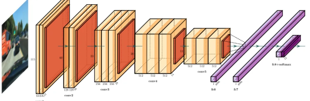
• After each convolution layer, non-linearity (e.g., ReLU) is applied. It is worth noting that a stack of two and three convolution layers produce an effective receptive field of 5×5 and 7×7, respectively. This design choice has some benefits. First, the VGG approach has made the decision function more discriminative by applying more non-linearity. For instance, the first convolutional layer has a filter-size of 7 × 7, followed by a non-linearity in AlexNet. In contrast, a stack of three convolutional layers followed by non-linearity after each layer is applied in VGG to achieve the same receptive field. Second, the number of model parameters is decreased by 44%. The convention of using a small-size filter to do classification tasks is used previ-ously, but due to less depth, the result is not efficient for large scale image datasets. Goodfellow et al. [10] have applied a deep CNNs to recognize street numbers and showed that depth has a real effect on efficiency and accuracy, and increased depth led to significant performance. Figure 2.13 illustrates the VGG16 architecture. 64 64112 115 conv1 128 12856 60 conv2 256 256 25628 33 conv3 512 512 512 14 20 conv4 512 512 512 7 13 conv5 14096 fc6 14096 fc7 1 fc8+softmax 12
Figure 2.13: The VGG16 architecture.
2.4.3
ResNet
As the neural network goes in-depth, the network training becomes prob-lematic. This is due to the vanishing gradient problem. Moreover, the model parameters increase in deep networks. Tuning a higher number of model pa-rameters may forge the network to train with a higher error rate. Microsoft
layers, which is eight times larger than VGG [32]. It has won the first prize in ILSVRC with a 3.57% error rate on the imagenet data set.
The authors have introduced a residual mapping technique to overcome the vanishing gradient problem. Figure 2.14 illustrates residual learning building blocks.
• In traditional convention, inputxgoes through a stack of convolutional layers and output a function H(x). In ResNet, the original input x is added with the output function’s result denoted as F(x) instead of the straight transformation. The way the original input is carried to the output is called an identity shortcut connection. Identity short-cut connection does not affect on the network by adding extra model parameters and computational complexity.
H(x) = F(x) +x
• The identity shortcut connection has been used in two different ways. If the input and the output are of the same dimension, the input is added directly with the output. When the dimension increases, authors have considered two options, i.e., identity mapping with extra zero entries padded for increasing dimensions and a 1 × 1 convolutional layer. In both cases, the stride of 2 is used due to the dissimilarity of dimensions. Residual learning eases the training process during the backward pass of backpropagation, which helps the gradient flow easily through the graphs by distributing it. According to the authors, optimizing the residual mapping is more relaxed than the unreferenced mapping [14].
3x3, n 3x3, n 3x3, m 3x3, m 3x3,/2, n 3x3, n 1x1, m 1x1,/2, n + + +
ReLU ReLU ReLU
ReLU ReLU ReLU
n channels n channels n channels
2.4.4
Network-in-Network
Network-in-Network (NiN) [22] is a novel deep network structure that re-places the conventional generalized linear model (GLM) by a universal func-tion approximator to enhance the model segregafunc-tion for local patches within the receptive field. In the standard convolutional network, the feature map is produced by the execution of linear layers followed by a non-linear acti-vation function. The convolution filter used in CNN is a generalized linear model (GLM) with a lower abstraction level. Replacing GLM by non-linear function approximator can enhance the level of abstraction.
In NiN, a multilayer perceptron (MLP) is used as a non-linear function approximator. The decision is made based on two reasons. First, the MLP is compatible with a convolutional neural network which is trained by back-propagation techniques. Second, the MLP itself is considered as a deep model. NiN is organized by several stacks of MLP convolutional layers followed by a global average pooling layers. It does not have any fully-connected layer at the end of the convolution layers. Instead, the spatial average of the feature map results in the confidence of categories . The global average pooling does the process. A softmax function is applied to the resulting vector after the pooling. Figure 2.15 represents a micro-network (MLP) based NiN structure, which has three MLP convolutional layers and one global average pooling layer.
Figure 2.15: The overall structure of Network-in-Network. Source: [22]
2.5
Recurrent Neural Networks (RNNs)
Recurrent Neural Networks are considered a class of neural networks which process data in a sequential order. The word recurrent means the same pro-cess is executed for each element of a sequence, and the output depends on the previous computation. Some researchers interpret the dependency pro-cess of RNNs as memory where information from the previous calculation
H H(0) H(1) H(t-1) H(t) W1 W3 W2 W1 W1 W1 W1 W2 W2 W2 W2 W3 W3 W3 W3 X X(0) X(1) X(t-1) X(t) .... ....
Figure 2.16: A general architecture of recurrent neural network. Source: [21]
Figure 2.16 represents an unrolled/unfolded recurrent neural network. For example, if the data represents a sentence and the sentence has five words, then the network will be unrolled into 5-layers, one layer for each word. The internal computation of the recurrent neural network works as follows:
• W1, W2, and W3 represent the model parameters or weights of the network. An interesting factor to notice is that all the layers share the same parameters across all steps that reduce the total number of model parameters to be learned.
• X(t) is the input at time step t. H(t) is the hidden state at time step
t. H(t) is calculated based the following formula H(t) =f(X(t)∗W1 +
H(t−1) ∗W2). Here, function represents the activation function (i.e.,
sigmoid, tanh and ReLU). The hidden state interprets as the memory of the network. The first hidden state H(−1) is set to all zeros.
• Y(t)is the output of corresponding inputX(t)at time stept. The output
at each time step depends on the application domain. It is not manda-tory to calculate output at each time step. For instance, predicting sentiments of a sentence.
The training process of recurrent neural networks is almost similar to the neural network with a slight difference. The backpropagation is called Backpropagation Through Time (BPTT) in RNNs as the gradient at each output depends not only on the calculations of t time step but also on the t−1 time step.
The general recurrent neural networks, which are also known as vanilla recurrent neural networks, face the vanishing gradient problem. The gradient is used to adjust the weights of the network. The adjustment depends on how the value of the gradient evolves. If the amount of the gradient is large, the impact of the weight adjustment is also significant, and if the value of the gradient decreases, it affects the weight adjustment. As the BPTT progresses, the gradient drastically shrinks, and the layers at the beginning of the network fail to learn as the weights are slightly adjusted due to a small gradient. This problem is called the vanishing gradient problem, and the network suffers from short-term memory.
There are two particular kinds of recurrent neural networks in practice, such as Long Short Term Memory networks [15] and Gated Recurrent Units [4] to mitigate the short-term memory of recurrent neural networks.
2.5.1
Long Short Term Memory (LSTM)
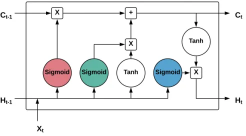
Long Short Term Memory (LSTM) is a special kind of recurrent neural net-work capable of learning long term dependencies. It has control flow like vanilla recurrent neural network with some additional functionalities, which helps to keep and remove information from the sequence data. LSTM also forms the chain of repeating modules similar to the vanilla recurrent neural networks. The illustration of LSTM building module is shown in Figure 2.17
• The horizontal line at the top of the figure is known as the cell state, which is the core component for ensuring long-term memory. LSTM can add new information and remove unnecessary old information in the cell state through the regulation of some gates.
• There are three gates responsible for protecting and controlling the cell state. The sigmoid function governs all the gates. The sigmoid function provides output between 0 and 1. If the output of thesigmoid function is close to zero, the information can be forgotten or removed. If the output is nearly 1, the information should be kept.
• The first gate is a forget gate. This gate decides what information should be kept or removed. The red color circle indicates the forget gate. The input of the current state Xtat time step t, and information
from the previous hidden state Ht−1 are merged and fed through the
forget gate. The output of the forget gate multiplies with the cell state to preserve valid information.
color circle represents the input gate. Ht−1 +Xt are passed through
a tanh function, which squishes the value between -1 to 1 to regulate the network. The input gate decides which information should be kept from the tanh function output and added to the cell state. Thus, the new information is added in the cell state.
• The third and the last gate is output gate, which generates the next hidden state information. The blue color circle denotes the output gate. Similar to the input gate,Ht−1+Xtare passed through an output
gate, and the newly modified cell state is passed through a tanh func-tion. Both outputs are multiplied to decide which information should be carried through the hidden state.
Sigmoid Sigmoid Tanh Sigmoid
X + X X Tanh Ht-1 Xt Ct-1 Ct Ht
Figure 2.17: Building module of LSTM.
2.5.2
Gated Recurrent Units (GRUs)
Gated Recurrent Unit (GRU) aims to solve the vanishing gradient prob-lem and work almost similar to the LSTM. GRU also has two gates that help coordinating the relevant information to pass through the chain of the GRU modules. The illustration of the GRU building module is shown in Figure 2.18.
• GRU has two gates, such as an update gate and a reset gate. The up-date gate helps to keep relevant information to pass through the GRU module, and the reset gate forgets irrelevant information to improve the prediction result. In Figure 2.18, green and red color circles indicate the update and the reset gate, respectively.
• The update gate uses the sigmoidfunction, which produces an output result between 0 and 1. Close to 0 means forget the information, and close to 1 indicates to keep the information. The output of the update gate is denoted as ut. Here,W1u andW2u represents the weights of the
input xt and the weights of the previous module’s information ht−1,
respectively. The equation of the update gate is given below. ut=σ(W1u.xt+W2u.ht−1)
• The reset gate works similar to the update gate as it also has the same activation function. The output of the reset gate is denoted as rt. Only the difference between the gates is corresponding weights and
usages. The equation of the reset gate is given below. rt=σ(W1r.xt+W2r.ht−1)
• The output of the reset gate introduces a candidate content that stores as relevant information from the previous hidden unit. The output of the reset (rt) and the product of the previous hidden unit (ht−1)
and its weights (W2) are element-wise multiplied to determine what
to remove from the previous time step. The tanh function is used to generate the output of current memory content. For instance, consider a smartphone review sentiment analysis problem. Some reviewer wrote, “The X phone has all the common features. . . . But the camera does not perform well, which I need most.” Here, the most relevant part of the review is in the last sentence, which means the previous information are not relevant to determine the reviewer’s satisfactory level. The general formula is given below.
h0t = tanh (W1.xt+rt∗W2.ht−1)
• In the final step, the result of the update gate is used to determine what information should be kept from the candidate contents and the previous hidden unit. Let us consider the previous example. The last sentence holds the relevant information. At this time step, the most
the candidate content should be ignored. The update gate helps to determine this by generating results close to 0 and 1. The formula for the hidden unit at time step t is given below.
ht =ut∗ht−1+ (1−ut)∗h 0 t Sigmoid Sigmoid tanh + + X + X X + ht-1 xt ht ht ut 1 - ut h't rt
Figure 2.18: Building module of GRUs.
2.6
Recursive Neural Networks (RNNs)
Recursive neural networks are non-linear adaptive models, which learn and predict based on the deep structured data. In the early ’90s, the neural net-works were successful while processing fixed-length data and variable-length sequences. Still, they cannot apply efficiently on structured data, such as the logical terms, trees, and graphs. Christoph Goller et al. [8] first presented a novel approach that was capable of solving inductive inference problems on complex symbolic structures of variable size. Since then, the researchers
are working to represent and classify structured data with the help of neu-ral networks. Sperduti et al. [34] have proposed an approach of geneneu-ralized recursive neurons, where all the supervised sequence classification networks can be generalized into structures. The authors have presented a framework to solve the problem of processing structured information [6].
The principle motivation behind the recursive neural networks is to work with the information of different sizes and topologies. In contrast, the feature-based approach works with a fixed-size data. A backpropagation technique is used, known as Backpropagation Through Structure (BPTS) to train a recursive neural network. Recursive structures are found in natural scenes and natural language sentences [33]. The authors have proposed a structure predicting algorithm based on a recursive neural network that parses natural scenes, natural language sentences and predicts with appropriate class labels. Figure 2.19 illustrates the parsing process of natural scene and sentence in RNNs.
Figure 2.19: Parsing natural scene and sentence in RNNs. Source: [33]
Advantages of recursive neural networks
• Robust against the vanishing gradient problem.
• Efficiently learn hierarchical, structured and variable length data. Disadvantages of recursive neural networks
• The hierarchical structure of every input data must be known while training.
• Difficult to work in mini-batches as the hierarchical structure changes for every training data.
Distributed DNN inference
Intelligent applications enable by advanced artificial intelligence solutions have been deployed in places ranging from homes to far away satellites. In fact, machine learning techniques allow to obtain high accuracy and reli-ability in several tasks, especially deep neural networks, natural language processing, image and voice recognition, and computer vision. Self-driving vehicles, smart assistant applications are some of the contributions of ad-vanced machine learning technologies. Deep neural networks (DNNs) require high computational resources to train and predict models. Today’s cloud technologies provide extensive resources for running DNN tasks. Heavy com-putation of intelligent applications are taking advantage of this cloud facili-ties. The main disadvantage of the cloud-only approach lies in transmitting a significant amount of data through the wireless communication channel with high latency. With the advancement of the powerful System on Chip, the end devices are becoming resourceful and capable of executing a DNN task. Moreover, researchers are also focusing on offloading the DNN tasks or parti-tioning DNNs to the neighboring edge/fog devices, which are relatively more potent than the end devices for accelerating DNN computation by alleviating device-level computing cost and memory usage. Generally, DNN inference is offloaded to the edge. A trained network (model) is used to predict/infer the test samples to predict the output in DNN inference. The rest of this chapter reviews research works in DNN inference acceleration that are more relevant.
3.1
Distributed mobile computing system
Most DNN applications are performed on client-server architecture due to adequate computing capability required for executing DNN tasks. Mao et
al. [23] have proposed a local distributed mobile computing system for DNN (MoDNN). This first work has considered heterogeneous mobile devices in a local cluster communicating over Wi-Fi.
The article has described the methodologies as follows. First, the authors have built a heterogeneous mobile computing cluster, connecting through Wi-Fi direct, a standard for peer-to-peer wireless communication, which has a high transfer rate (∼ 250 Mbps) compared to a cellular network. Second, two layer-aware partitioning schemes have been proposed. Most state-of-the-art DNN architectures are designed by the convolutional layers, followed by the fully-connected layers. The convolutional layers are computing-intensive, whereas the fully-connected layers consume excessive memory. Based on ex-periments, authors have observed that the convolutional layer’s computing cost depends on the size of the input, and the number of weights affects the memory usages in case of the fully connected layers. They have proposed a Biased One-Dimensional Partition (BODP) based on computing capabil-ities of mobile devices for partitioning the convolutional layers. A weight partitioning algorithm is introduced to partition the fully-connected layers inspired by the spectral clustering techniques which cluster the network using the eigenvalues of the similarity matrix of the data. Finally, the authors have implemented a scheduler for each mobile device as a middleware to plan the overall execution process.
The implementation is accomplished on the MXNet deep learning frame-work. The authors have used the VGG16 pre-trained DNN model, which is a very popular image recognition algorithm. The evaluation report of MoDNN suggests that the execution time decreases significantly based on the increas-ing number of worker nodes (mobile devices). The execution time improves by 2.17–4.28 times when the number of worker nodes increases from two to four. Figure 3.1 overviews the distributed mobile computing system.
3.2
Neurosurgeon
Kang et al. [18] have investigated both cloud-only execution and computa-tion particomputa-tioning methodology between the end devices and the cloud infras-tructure. They have experimented with eight intelligent applications in the domain of computer vision and natural language processing. They have also designed a scheduler that automatically partitions the DNN computation to find the best computation time and communication latency.
In the cloud-only approach, the authors have offloaded DNN computa-tion to the cloud infrastructure through a wireless communicacomputa-tion medium. The Jetson TK1 mobile platform is used as an end device, and a powerful
Figure 3.1: An overview of distributed mobile computing system.
computer equipped with a high performing GPU is used as a server. They have also experimented with DNN task execution in the mobile/end devices. The cloud processing has a higher computation impact than the mobile/end devices, but the communication latency is significantly high. Communica-tion latency varies based on transmitted data size. As the end devices are getting smarter and resourceful every day, DNN task execution achieves sig-nificant improvement, but often leads to extreme energy consumption. The cloud-only processing provides significant computation efficiency over mo-bile processing and achieves better performance with a fast communication medium.
Fine-grained computation partitioning is another approach proposed by the authors. The DNN computation is partitioned between the end/mo-bile device and the cloud. They have analyzed the computation behavior of popular DNN architectures at the layer granularity. Most state-of-the-art DNN architectures are formed based on conventional layers, such as fully connected, convolutional and pooling. Some additional computations are per-formed to provide more accuracy, such as normalization, softmax, argmax, and dropout. Authors have partitioned the DNN architectures to execute some of the layers on the end/mobile platform and the rest on the cloud in-frastructure. Based on the observations, the fully-connected layers are most costly with respect to computation time than other layers. It is also observed that the best partition point depends on the DNN architectures and appli-cation areas. For instance, a computer vision appliappli-cation provides the best
efficiency if the partitioning point is in the middle of the DNN, but in the case of speech recognition and natural language processing, partitioning at the beginning or the end is more suitable.
The best efficient point of partition depends mostly on the topology of the architecture. However, some other factors also affect the partitioning point, such as the state of the wireless medium and the cloud infrastructure load factor. The wireless medium has a variance, which affects the transmission latency. Therefore, the query service time gets increased due to the load pat-tern of the data center. Considering the above aspect, authors have proposed an intelligent DNN partitioning engine called Neurosurgeon, which selects the best partitioning point to optimize computation, communication latency, and energy consumption. Neurosurgeon consists of two phases, such as deploy-ment phase and runtime phase. The deploydeploy-ment phase generates a prediction model by profiling the end/mobile devices and the server. The information is stored in the mobile devices for future prediction of latency and energy cost of each layer. In the runtime phase, four steps are performed. First, analyzing and extracting the DNN layer configurations. Second, predicting layer performance from the layer prediction model. Third, evaluating the partition point considering the wireless bandwidth and the server load, and finally, executing the DNN partition between the end/mobile platform and the server/cloud. Figure 3.2 illustrates the overview of the Neurosurgeon.
Figure 3.2: An overview of the Neurosurgeon. Source: [18]
3.3
DNN Surgery
Hu et al. [16] have proposed a framework, Dynamic Adaptive DNN Surgery (DADS), that supports partitioning the DNN architectures between the edge and the cloud.
While designing the DNN Surgery, authors have given importance to two aspects. First, the dynamic behavior of communication networks, and
sec-creases due to the massive amount of traffic in the LTE (4G) network. On the contrary, the computation latency increases under high throughput condi-tions. The best possible cut decision needs to be ensured considering both the scenarios. In the case of peak hours, the layer with a smaller data size than the input is considered as partition point. The DNN computation is partitioned at the input layer during the higher network capacity period. Another con-cerning issue is that recent DNN architectures are based on directed acyclic graphs (DAGs) topology instead of chain topology. Partitioning the DAG topology needs more graph-theoretic analysis than the chain topology lead-ing to the NP-hard problem. To mitigate both the network and the topology problem, authors have proposed two adaptive dynamic schemes, such as DNN Surgery Light (DSL) and DNN Surgery Heavy (DSH). The proposed DADS continuously monitors the network condition and decides which scheme is ap-propriate for the current state. If the network is in a lightly loaded condition, the DSL is applied; otherwise, the DHL is suitable for heavily loaded condi-tions. The DSL’s primary goal is to minimize the overall delay to process one frame, and the DHL aims to maximize the throughput. To reduce the overall delay, the problem is converted into a min-cut problem to find the globally optimal solution. Figure 3.3 shows the conversion of the min-cut problem. An approximation approach is applied to solve the NP-hard problem, which is not solvable in polynomial computational complexity.
Input 3 x 3 Conv 3 x 3 Conv Avg Pooling V1 V2 V3 V4 V'1 V2 V3 V4 V1 Edge Cloud Cut
Layer representation Graph representation
Conversion to minimum s-t cut problem
Figure 3.3: The conversion to the min-cut problem. Source: [16]
Authors use Raspberry pi 3 model B as the edge device and Cloud Ali as the cloud. The client-server interface is implemented using the gRPC pro-tocol. The edge device extracts the sample frame from the self-driving car
video data set. The edge also makes the partition decision based on the net-work condition and accordingly processes the allocated layers. The partition decision and the intermediate results are transmitted to the cloud after the execution phase at the edge. The cloud receives the partition decision and executes the rest of the computation. The DNN surgery is compared with the edge-only and the cloud-only approaches. This technique has a com-putation latency speedup of 6 and 8 times (approx.) compared with the edge-only and the cloud-only approaches, respectively. In terms of through-put gain, it has a speedup of 8 and 11 times (approx.) compared with the other two approaches. The work also compares with Neurosurgeon [18]. The DNN surgery and the Neurosurgeon perform equally in the chain topology, but the DNN surgery outperforms the Neurosurgeon in heavy workload con-dition. The overall argument of this research suggests that if the network provides a high bandwidth and a high data rate, it is advisable to offload the large portion of the DNN computation to the cloud for better performance. The edge-only approach is feasible only in low data rate conditions.
3.4
Distributed deep neural network
Distributed Deep Neural Network (DDNN) [38] is a framework over dis-tributed computing hierarchy, which consists of the disdis-tributed end devices (local network), the edge, and the cloud. A single end-to-end DNN model is jointly trained by the framework over three-tier (i.e., a local network, the edge, and the cloud) for fast and efficient localized inference with better prediction confidence.
In conventional distributed DNN computation, a small neural network (NN) model is executed in the end devices for initial feature extraction, and a large NN model is executed in the cloud for more robust feature extraction and classification. These approaches need to encounter some challenges, such as limited computation capability of resource-constrained devices due to in-sufficient memory and low battery power, aggregation of sensor data from multiple end devices for a single DNN task execution, and joint training of the models on the end devices, the edge, and the cloud. Teerapittayanon et al. [38] have proposed a framework that is capable of mapping sections of a DNN over distributed computing hierarchy, training a DNN model in a dis-tributed manner, and allowing automatic sensor fusion through aggregation schemes. The DDNN framework has exit points defining the sample classifi-cation at earlier points in a NN. In the distributed environment, the DDNN framework has three exit points, e.g., local exit, edge exit, and cloud exit. When a classification task achieves a certain level of prediction confidence on
with multiple geographically distributed end devices, and edge networks, which are aggregated together for performing classification tasks. Authors have presented three approaches for aggregating the output of the end de-vices or the edge networks: Max pooling (MP), Average pooling (AP), and Concatenation (CC). The joint training follows the GoogleNet [37] training process. During the back-propagation phase, the calculated loss from each exit point is accumulated together to train the entire network jointly.
The DDNN reduces communication cost 20×compared to offloading raw sensor data from the end devices to the cloud.
Figure 3.4: An overview of distributed deep neural network framework. Source: [38]
3.5
Distributed inference acceleration (DINA)
This thesis has implemented a DNN adaptive task partitioning and offload-ing approach based on the research paper by Mohammed et al. [25], whichis inspired by the recent contributions in the DNN inference acceleration mentioned above.
Most of recent approaches split the DNN into two parts: one part ex-ecutes on the end or edge device, and the other part on the cloud. These approaches have some trade-off between computation time and transmission time. Mohammed et al. [25] have proposed a technique to split the DNN computation into multiple partitions that can be processed locally on end devices or distributed the partitions across one or multiple fog nodes in a network. Authors have introduced two schemes: an adaptive DNN partition and a distributed algorithm based on matching theory to offload the DNN. Figure 3.5 overviews the underlying model. In Figure 3.5 (a), the DNN in-ference task di divides into sub-tasks (i.e., v0, v1, . . . , vn). The sub-tasks are
the DNN layers in the context of the DNN inference. Moreover, the sub-task can be partitioned into more smaller tasks (i.e., vi =vi0, vi1, . . . , vin). These
sub-divided tasks are then offloaded to the neighboring fog nodes selected based on the utilities shown in Figure 3.5 (b).
DNN inference taskd1 a1 a1 a 2 a1 a6 a1 v21 v22 v23 a3 a1 a4 a1 a5 a1 v0 v1 v3 Sub-task Layer (a) d1 a1 a1 a 2 a1 a 6 a1 v21 v22 v23 a4 a1 v0 v1 v3 Fog node f1 Fog node f2 Fog node f3 User node u1 REV 1.2 2011-0 8-08 ____ Other user nodes a5 a1 a3 a1 (b)
Figure 3.5: An overview of the DINA. Source: [25]
Mohammed et al. [25] have presented Distributed INference Acceleration (DINA), which is based on a matching game approach. The matching game theory, also known as search and matching theory, is an arithmetical frame-work introduced in economics. This theory describes the relational behavior between two sets of entities with preferences on each other [30]. It has been applied in wireless networking for resource allocation [13]. The significant contribution of this work is given below. All the notations are summarized in Table 3.1.
F Set of fog nodes
A Set of DNN layers/partitions ϕf a Service utility of fog node f
ϕuf Service utility of user node u
u Preference relation of user node u
f Preference relation of fog node f
µu Preference list of user node u
ruf Data rate of user node u towards fog node f
xf a Binary variable denoting task a assigned to fog node f
τa Delay threshold for task a
δ Edge delay
θ Maximum fog nodes for offloading Γ Target transmission rate threshold
Tf a Total execution time for task a at fog nodef
Ttr
f a Transmission time for task a to fog node f
Texe
f a Execution time for task a at fog nodef
Tf aque Queuing time for task a at fog node f
Tquef a Average queuing time for task a at fog node f Table 3.1: Summary of notations.
3.5.1
Fine-grained adaptive partitioning (DINA-P)
The DNN task is divided into multiple fragments that are smaller than a single layer. The partitioning scheme considers the specific characteristics of layer types in different DNN architectures and represents the partition into a matrix to reduce communication overhead.
The partitioning algorithm is called DINA-P and relies on utility functions for both user nodes and fog nodes. The utility of a fog node denoted as f for executing a task denoted as a of a user node denoted as u is:
ϕf a =xf a(t)(τa−Tf atr −T exe f a −T
que
f a ) (3.1)
whereτarepresents the delay threshold for taska. Tf atr is the transmission
time for taska to fog nodef and Texe
f a is the execution time for task a at fog
node f. Tquef a denotes the average queuing latency. xf a ∈ {0,1} is a binary
variable defines the offloading problem.
ϕuf = 1 Tf a (3.2) Tf a =Tf atr +T exe f a +T que f a +δ (3.3)
where Tf a denotes total execution time for task a at fog node f and δ is
the edge delay. Table 3.1 summarizes the notations. Algorithm 1: Adaptive DNN partitioning (DINA-P)
Input :p: convolution kernel size; ϕf a: utility of f;|fn|: number of fog
neighborsf ofu∈ U;G: DAG for DNN inference taskd;
Rm×n
a: matrix associated with subtask a,∀a∈ A;c: compute
power off.
Output :DNN partitionsP ={P1, P2, P3, . . .}
Init :P ← ∅,c0= 0, w←max(m, n)
1 forallabelonging to parallel paths inG
2 fori∈[1,|fn|+ 1