High Performance Parallel Algorithms for the Tucker
Decomposition of Sparse Tensors
Oguz Kaya, Bora U¸car
To cite this version:
Oguz Kaya, Bora U¸car. High Performance Parallel Algorithms for the Tucker Decomposition of
Sparse Tensors. International Conference on Parallel Processing (ICPP), Aug 2016, 2016-08-19,
United States. ICPP 2016, 2016.
<hal-01354894>
HAL Id: hal-01354894
https://hal.inria.fr/hal-01354894
Submitted on 19 Aug 2016
HAL
is a multi-disciplinary open access
archive for the deposit and dissemination of
sci-entific research documents, whether they are
pub-lished or not.
The documents may come from
teaching and research institutions in France or
abroad, or from public or private research centers.
L’archive ouverte pluridisciplinaire
HAL
, est
destin´
ee au d´
epˆ
ot et `
a la diffusion de documents
scientifiques de niveau recherche, publi´
es ou non,
´
emanant des ´
etablissements d’enseignement et de
recherche fran¸cais ou ´
etrangers, des laboratoires
publics ou priv´
es.
High Performance Parallel Algorithms
for the Tucker Decomposition of Sparse Tensors
Oguz KayaINRIA and LIP, ENS Lyon Lyon, France [email protected]
Bora Uc¸ar
CNRS and LIP, ENS Lyon Lyon, France [email protected]
Abstract—We investigate an efficient parallelization of a class of algorithms for the well-known Tucker decomposition of general N-dimensional sparse tensors. The targeted algorithms are iterative and use the alternating least squares method. At each iteration, for each dimension of an N-dimensional input tensor, the following operations are performed: (i) the tensor is multiplied with(N−1)matrices (TTMc step); (ii) the product is then converted to a matrix; and (iii) a few leading left singular vectors of the resulting matrix are computed (TRSVD step) to update one of the matrices for the next TTMc step. We propose an efficient parallelization of these algorithms for the current parallel platforms with multicore nodes. We discuss a set of preprocessing steps which takes all computational decisions out of the main iteration of the algorithm and provides an intuitive shared-memory parallelism for the TTM and TRSVD steps. We propose a coarse and a fine-grain parallel algorithm in a distributed memory environment, investigate data dependencies, and identify efficient communication schemes. We demonstrate how the computation of singular vectors in the TRSVD step can be carried out efficiently following the TTMc step. Finally, we develop a hybrid MPI-OpenMP implementation of the overall algorithm and report scalability results on up to 4096 cores on 256 nodes of an IBM BlueGene/Q supercomputer.
Keywords-sparse tensors, parallel tensor factorization, Tucker decomposition, higher order orthogonal iteration
I. INTRODUCTION
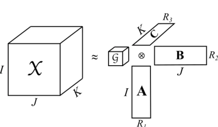
Tensors or multi-dimensional arrays are used to represent data with high dimensionality in many applications. Among the most popular of these applications are the analysis of Web graphs [1], forming knowledge bases [2], [3], item and tag recommendations [4], [5], [6], chemometrics [7], signal processing [8], computer vision [9], and forensic data analy-sis [10]. In these applications, tensor decomposition algorithms are used to find latent relations or predict missing elements in the data using its low rank structure. There are two prominent tensor decomposition formulations.CANDECOMP/PARAFAC (CP)decomposition formulates a tensor as a sum of rank-one tensors. Tuckerformulation expresses a tensor with a smaller core tensor multiplied by a matrix along each dimension—see Fig. 1 for a simplistic view. Both of these formulations have uses in various applications; in particular, the CP formula-tion is deemed useful for understanding latent components, whereas the Tucker formulation is considered to be more appropriate for compression [11], identifying relations among the factors [12], and predicting missing data entries [4]. Tucker
A
C
⊗B
≈
I
J
K
X
I
K
J
G
R
1R
2R
3Fig. 1: Tucker decomposition of a 3rd mode tensor X ∈ RI1×I2×I3 as a core tensor G ∈
RR1×R2×R3 multiplied by
matrices A ∈ RI1×R1, B ∈
RI2×R2 and C ∈
RI3×R3 in
different modes. In the CP-decomposition, G is a diagonal tensor having the same size along each dimension, andA,B andChave the same number of columns.
decomposition and its variants are known to be more effective tools for data analysis at the expense of higher computational requirements, and many of its variants have been employed in data analysis problems [4], [5], [6]. In these applications, the tensor formed from the data is sparse, which can adequately be exploited to compute the Tucker decomposition more efficiently. With this motivation, we investigate the efficient parallel computation of the low rank Tucker decomposition of sparse tensors in shared and distributed memory environments. There are variants of CP and Tucker decompositions, and different algorithms to compute them [13], [14]. The most common algorithms for both decompositions and their variants are based on the alternating least squares (ALS) method. The algorithms of this type are iterative, where the computational core of an iteration is a special operation performed on anN -mode tensor andN matrices. The key operation in the ALS-based CP decomposition (CP-ALS) case is called the matri-cized tensor times Khatri-Rao product; we refer the reader to other resources for details [14]. The key operation in the ALS-based Tucker decomposition algorithm, namely Higher Order Orthogonal Iteration (HOOI) [15], is called tensor times matrix-chainproduct. These two operations pose similar computational challenges; but there are distinct opportunities for parallel efficiency.
algorithm is performed for all modes of the N-mode input tensor in sequence, at every ALS iteration. TTMc for a mode n involves tensor times matrix (TTM) products with N −1 different matrices, each of which is associated with one of the modes other than n. TTM product can be considered as a higher dimensional variant of the matrix-vector multiply operation (Section II explains the TTM operation in detail). Techniques for efficiency of a single TTM are therefore akin to those used in the matrix-vector multiplication but require more effort to overcome the difficulties associated with the higher dimensionality.
Following the TTMc step for each mode, HOOI algorithm computes a few singular vectors of a large, usually tall-and-skinny dense matrix at every ALS iteration. This matrix arises from a logical reorganization of the result of the TTMc asso-ciated with the corresponding mode. The cost of computing the singular vectors is not negligible and hence needs to be addressed in an efficient parallelization of the HOOI algorithm. We refer to the computation of the desired singular vectors as the truncated SVD (TRSVD) step.
Our contributions are as follows. First, we design efficient parallel algorithms for the TTMc operation on sparse tensors. To this end, we first introduce a particular nonzero-based refor-mulation of TTMc. Using this forrefor-mulation, we then introduce a preprocessing step called symbolic TTMc to identify data dependencies and perform all index computations before the HOOI iterations for efficiency. Then, we provide a shared-memory parallel algorithm for the main iteration of HOOI which makes use of the symbolic TTMc step. Second, we introduce a coarse and a fine-grain task definition for TTMc and TRSVD steps within the HOOI algorithm, and propose a hybrid shared-distributed memory parallel algorithm based on the distribution of these tasks. We discuss the computational and communication requirements of the algorithm for a given task distribution, and make use of the hypergraph models from our earlier work on CP-ALS [16] for reducing communication and achieving load balance during each HOOI iteration. Third, we stress how to efficiently perform the TRSVD step in a distributed memory setting, and make use of the PETSc [17] and SLEPc [18] libraries in this step. We carefully designed this step so that the communication requirements in parallel iterative algorithms used for computing the singular vectors are reduced, and the load balance is achieved by making use of the data decomposition of the TTMc step. Finally, we propose an efficient OpenMP-MPI hybrid parallel implementation of the HOOI algorithm in C++, and present scalability results on a high-end parallel system using up to 4096 cores on real world tensors. To the best of our knowledge, this is the first high performance parallel implementation of the HOOI algorithm for sparse tensors in shared/distributed memory environments using OpenMP/MPI.
The organization is as follows. We give background on the basic tensor operations, and a reformulation of the TTMc operation for sparse tensors in the next section. Then, in Section III, we propose shared and distributed memory parallel HOOI algorithms and discuss in detail the TTMc and the
TRSVD steps. Next, we give a brief summary of related recent work in Section IV. Finally, we provide experimental results in Section V, and conclude the paper in Section VI.
II. BACKGROUND
We use bold, upper case Roman letters for matrices, as inA. Matrix elements are shown with the corresponding lowercase letters, as inai,j. Matlab notation is used to refer to the entire
rows and columns of a matrix, e.g.,A(i,:)andA(:, j)refer to theith row andjth column of A, respectively.
We use calligraphic fonts to refer to tensors, e.g.,X. The
orderof a tensor is the number of its dimensions or modes, which we denote with N. For the sake of simplicity of the notation and the discussion, we sometimes discuss the case N = 3, even though our algorithms and implementations have no such restriction. We explicitly generalize the discussion to order-N tensors whenever necessary. As in matrices, an element of a tensor is denoted by a lowercase letter and subscripts corresponding to the indices of the element, e.g., the element(i, j, k)ofXisxi,j,k. Afiberof a tensor is defined by
fixing every index but one, and aslice of a tensor is obtained by fixing only one index. For instance, for a third order tensor X,X:,j,k andXi,j,: are fibers and Xi,:,: and X:,:,k are slices
in the first and the third modes, respectively.
TheKronecker product of two vectorsu∈RI andv∈RJ results in a vectorw=u⊗vwherew∈RIJ andwj+(i−1)J =
uivj. We denote theouter productof the same vectorsuand
v as W = u◦v, where W ∈ RI×J and wi,j = uivj. In
general, performing the outer product ofN vectors produces anN-dimensional tensor.
We reproduce the following definitions from Kolda and Bader’s survey [14]. Then-modematricizationof a tensorXis denoted byX(n)and refers to the reordering of X’s elements
into a matrix by arranging the mode-nfibers as the columns of X(n). For example, forX∈RI1×···×IN,X
(1)∈RI1×(I2···IN)
denotes the mode-1 matricization ofX, where the rows ofX(1)
correspond to the first mode ofX, and the columns correspond to the remaining modes. The tensor element xi1,...,iN
corre-sponds to the elementi1,1 +P
N j=2 h (ij−1)Q j−1 k=1Ik i of X(1).
The n-mode product of a tensor X ∈ RI1×···×IN with a
matrixU∈RJ×Inis denoted byX×
nU. This is also referred
to as tensor times matrix (TTM) product. The result Y is a tensor of size I1× · · · ×In−1 ×J ×In+1× · · · ×IN. A
particular element of Yis given by yi1,...,in−1,j,in+1,...,iN =
In
X
in=1
xi1,i2,...,iNujin . (1)
A tensor can be multiplied by a set of matrices along a given setSof modes. We use the notation TTMc(X, S,{Un:
for n∈S})to refer to the tensorn-mode product of Xwith matrices Un for n ∈ S. We use TTMc(S) for clarity, as
the tensor X and the matrices Un’s will be clear from the
context. The operation Y← X×1U1· · · ×n−1Un−1×n+1
except n, which we denote as X×−n Un, or equivalently,
TTMc({1. . . N} \ {n}).
The Tucker decomposition expresses a given tensor X ∈ RI1×···×IN as a core tensor G multiplied by a factor matrix
Unof sizeIn×Rnin each moden. Here,R1, . . . , RN are the
requested rank of the decomposition for each mode. Formally, the Tucker decomposition[[G;U1, . . . ,UN]]writesXasG×1
U1×2· · · ×N UN. For example, if X ∈ RI1×I2×I3, then
in its Tucker decomposition [[G;A,B,C]] we have xi,j,k ≈
PI1 p=1 PI2 q=1 PI3 r=1gpqraipbjqckr.
A well-known algorithm for computing the Tucker de-composition is called the higher order orthogonal iteration (HOOI) [19], and is given in Algorithm 1. In this algorithm, the factor matrices are initialized first. This initialization could be done randomly or using the higher-order SVD [19]. Then, the “repeat-until” loop applies the alternating least squares method. Here, for each mode n, TTMc({1, . . . , N} \ {n})at Line 4 is computed. This produces a tensor of sizeR1×R2×
· · · ×Rn−1×In×Rn+1× · · · ×RN, which is then matricized
along thenth mode into the matrixY(n)∈RIn×Πi6=nRi. Then, the leadingRn left singular vectors ofY(n)are computed and
used as the columns of Un at Line 5. After all matrices Un
are updated, the core tensor G is formed at Line 6, and the change in the fit measure (|X| − |G|)/|X| is checked at the end of each iteration.
Algorithm 1 HOOI algorithm forN-mode tensors Input: X: AnN-mode tensor
R1, . . . , RN:
The rank of the decomposition for each mode
Output: Tucker decomposition[[G;U1, . . . ,UN]]
1: Initialize the matrixUn∈RIn×Rn forn= 1, . . . , N
2: repeat
3: forn= 1, . . . , N do 4: Y←X×−nUTn
5: Un←Rnleading left singular vectors ofY(n)
6: G←X×1UT1 ×2· · · ×NUTN
7: untilno improvement or maximum iterations reached
8: return [[G;U1, . . . ,UN]]
How to perform the TTMc operation at Line 4 is especially important. These TTM’s can be performed in any order [14] using various schemes [20] that formulate TTMc in terms of multiple tensor-times-vector (TTV) operations. We now formulate TTMc in a way that specifies what to compute for each nonzero xi1,...,iN ∈X to be able to express parallelism
with different task granularities. Let Z = X×2UT2 where
X∈RI1×I2×I3, andU
2∈RI2×J2. By considering (1) forZ,
and performing the summation over nonzeros we obtain:
zi,t,k =
X
xi,j,k∈X
xi,j,kU2(j, t). (2)
We can vectorize this as Z(i,:, k) = X
xi,j,k∈X
xi,j,kU2(j,:). (3)
Similarly, Y=Z×3UT3 whereU3 ∈RI3×J3 can be written
as:
yi,m,t =
X
zi,m,k∈Z
zi,m,kU3(k, t).
Rewriting zi,m,k as in (2) we get
yi,m,t =
X
xi,j,k∈Z
xi,j,kU2(j, m)U3(k, t),
and finally by applying (3) twice we obtain Y(i,:,:) = X
xi,j,k∈X
xi,j,kU2(j,:)◦U3(k,:).
Specifically, for each nonzero xi,j,k ∈ X, we perform the
outer productU2(j,:)◦U3(k,:), scale it withxi,j,k, and then
add the result to the J2×J3 dense matrix Y(i,:,:). Using
the matricization of Y in the first mode, this results in the following formula where a Kronecker product replaces the outer product:
Y(1)(i,:) = X
xi,j,k∈X
xi,j,kU2(j,:)⊗U3(k,:). (4)
ForN-dimensional case, the formulation (4) generalizes to Y(n)(in,:) =
X
xi1,...,in,...,iN∈X
xi1,i2,...,iN ⊗t6=nUt(it,:)
where ⊗t6=n denotes the Kronecker product of N −1 row
vectors Ut(it,:) for t ∈ {1, . . . , N} \ {n}. This formulation
specifies the operations performed for each nonzero element of a tensor. The resulting computation of TTMc is called nonzero-based and is given in Algorithm 2 for 3rd order tensors andn= 1.
Algorithm 2 Nonzero-based formulation for the mode-1 ma-tricization of the TTMc operation Y=X×2UT2 ×3UT3 for
3rd order tensors
Y(1)←0
for allxi,j,k∈Xdo
Y(1)(i,:)←Y(1)(i,:) +xi,j,k(U2(j,:)⊗U3(k,:))
III. PARALLELTUCKERFACTORIZATION
An efficient shared memory parallelization of the TTMc operation given in Algorithm 2 should avoid expensive lock mechanisms to resolve data dependencies. We perform a preprocessing step to organize the computations in a way that the subsequent numeric computations can be performed in parallel without any write conflicts. Following the TTMc step, computing the TRSVD of the matricized tensor Y(n)
requires special attention. Direct SVD methods that are em-ployed to compute TRSVD in dense Tucker decomposition algorithms are not feasible for sparse Tucker decomposition due to computational and memory constraints. For this reason, we resort to iterative methods for TRSVD, which not only reduces the computational cost by exploiting the low rank of
approximation, but also renders the memory overhead due to TRSVD computation almost negligible.
For the distributed memory parallelism, we employ coarse and fine-grain task definitions. A coarse-grain task corresponds to computing a particular rowY(n)(i,:)of the TTMc result, as
well as the corresponding rowUn(i,:)of the factor matrix
us-ing TRSVD. In this scenario, the owner of this task possesses all the tensor nonzerosxi1,...,iN wherein=i. Also, each such
nonzero implies data dependencies to the tasks corresponding to the rowsU1(i1,:), . . . ,UN(iN,:)to be able to perform the
computation of Y(n)(i,:)using Algorithm 2. Fine-grain task
definition relaxes this constraint by allowing nonzeros to be distributed freely. It associates each nonzero xi1,...,iN with a
task which is responsible to compute xi1,...,iN ⊗t6=nU(it,:)
and generate a partial result for Y(n)(in,:) of sizeQt6=nRt.
This size is exponential in the ranks of approximation; there-fore, merging the partial results can get very expensive in terms of communication, hence should be avoided. For this reason, we propose a novel method to effectively handle this communication within the TRSVD step.
A. Shared memory parallelism
1) Parallel TTMc: As shown in Algorithm 2, each nonzero xi,j,kcontributes an outer product toY(1)(i,:), or equivalently,
Y(i,:,:)while performing TTMc in the first mode. For shared memory parallelism, this poses a write conflict whenever two threads simultaneously process nonzeros whose first index are i. To resolve this, we make a pass over the data to compute an update list ul1(i) that holds the list of nonzeros xi,j,k
that will contribute toY(1)(i,:). In the actual implementation,
we only store the index t of the nonzero x(t) = xi,j,k to
avoid duplicating the nonzero within ul1(i). In this way, we
untangle the write conflicts for each row of Y(1) and avoid
using lock mechanisms. We also store the setJ1of all indices
i ∈ I1 such that ul1(i) 6=∅. We repeat this computation in
all dimensions, and name this step as symbolic TTMc, as it resolves all the index computations and dependencies once and for all outside the main loop of HOOI (shown at Lines 1-2 of Algorithm 3). This symbolic data can be reused many times for fasternumeric TTMcs within the main loop of HOOI. Finally, symbolic TTMc of each dimension can be performed independently; hence, we perform this computation in parallel in each dimension.
After the symbolic TTMc, each row i of Y(1) can be
updated independently in parallel by using ul1(i), which
composes the parallel numeric TTMc step at Lines 5–8 of Algorithm 3. In our implementation, we use OpenMP parallel loop with dynamic scheduling to distribute the tasks to threads.
2) Parallel truncated SVD: Following the TTMc prod-uct for mode n, HOOI requires finding the leading Rn
singular vectors of the matricized tensor Y(n) to update
the matrix Un for mode n. Here, Y(n) is of size In ×
(R1· · ·Rn−1Rn+1· · ·RN). In Algorithm 3, we directly
com-pute the matricized tensor and avoid the cost of matricization. In a recent work on parallel Tucker decomposition of dense tensors [11], leading singular vectors ofY(n)are extracted by
Algorithm 3 Shared memory parallel HOOI Input: X: AnN-mode tensor
U1, . . . ,UN: Initial factor matrices
R1, . . . , RN: Ranks of approximation
Output: [[G;U1, . . . ,UN]]: Tucker approximation ofX
1: parforn= 1toN do
2: {uln, Jn} ←SymbolicTTMc(X,{1, . . . , N} \ {n})
3: repeat
4: forn= 1 toN do
5: parfori∈Jndo ITTMc for mode n
6: Y(n)(i,:)←0
7: for allxi1,...,iN ∈uln(i)do
8: Y(n)(i,:) +=xi1,...,iN[⊗t6=nUt(it,:)]
9: Un←TRSVD(Y(n), Rn)
10: G←Y×NUN
11: untilconvergence or maximum number of iterations reached
12: return [[G;U1, . . . ,UN]]
computing the eigenvalues of the Gram matrix Y(n)Y(n)T,
where the number of rows ofY(n), which is In, is typically
in the order of a thousand. However,In can easily exceed a
million for sparse tensors, rendering this method impractical for our purpose. Also, direct methods for eigenvalue and singular value problems typically compute all eigen/singular values at once, whereas in HOOI we need only Rn left
leading singular value/vector pairs out ofmin(In,Qi6=nRi).
For these reasons, we resort to using matrix-free iterative methods to compute the TRSVD of Y(n) [18]. This way,
we avoid forming the Gram matrix and compute only the required singular value/vector pairs. In the shared memory context, this TRSVD can be parallelized by using optimized BLAS2 gemv kernel for the matrix-vector (MxV) and matrix transpose-vector (MTxV) multiplications, which dominate the computational cost of the TRSVD due to the matrix being dense. As we demonstrate in the next section, this approach also enables us to reduce the communication requirements in the distributed memory setting.
After all factor matrices are updated, the core tensor is formed at Line 10 to check the convergence. Since atn=N, Y(n)already holds the TTMc resultY=X×1U1×2· · ·×N−1
UN−1 in the matricized form, we multiply Y with UN in
mode N to obtainG. Both Y andG are dense tensors while G being significantly smaller than Y (R1 × · · · ×RN vs.
R1× · · · ×RN−1×IN). The parallel computation of dense
Gcan efficiently be performed using BLAS3, and in practice its cost should be negligible compared to the cost of sparse irregular operations carried out in computingY. We skip the details of the parallelization of Line 10 and refer the reader to a recent work by Li et al. [21].
B. Distributed memory parallelism
1) Coarse-grain parallel HOOI: Recall that there are two main operations for each mode n in an iteration of HOOI: a TTMc step to obtain a matricized tensorY(n), and an TRSVD
step to obtain the matrixUn, onceY(n)is ready. In the
coarse-grain task decomposition of these computations, we define computing each row i of Un as an atomic task, and hold
the owner of this task responsible for computing the ith row ofY(n). We denote this task bytni, and make the owner oftni
own the corresponding data elements Un(i,:)andY(n)(i,:).
For each mode n, we partition these tasks. As a result, the process pk owns the index set Ink of tasks so that for each
i∈Ik
n,tni is owned bypk.
In Algorithm 2, Y(1)(i,:) receives a contribution
xi,j,k(U2(j,:)⊗U3(k,:))for each nonzeroxi,j,k. Therefore,
t1
i needs all nonzeros in the tensor slice X(i,:,:), as well
as the corresponding rows U2(j,:) and U3(k,:) to perform
the Kronecker product. To compute Y(1)(i,:), t1i involves
|X(i,:,:)| Kronecker products due to TTMc. During this computation, for each nonzeroxi,j,k,t1i needs the data owned
byt2j andt3k to perform the Kronecker product. This specifies the data to be exchanged in the communication step.
Algorithm 4 Distributed memory parallel HOOI executed at processpk
Input: Xk: Partition ofXowned by the processp k
type: ’coarse-grain’ or ’fine-grain’
I1k, . . . , I
k
N: Set of task indices owned bypk in each mode
U1, . . . ,UN: Initial factor matrices
R1, . . . , RN: Ranks of approximation
Output: [[G;U1, . . . ,UN]]: Tucker approximation ofX
1: parforn= 1toN do
2: {uln, Jn} ←SymbolicTTMc(Xk,{1, . . . , N} \ {n})
3: iftype=’coarse-grain’ then 4: Kn←Ink
5: else 6: Kn←Jn
7: repeat
8: forn= 1toN do
9: parfor alli∈Kn do ITTMc for moden
10: Y(n)(i,:)←0
11: for allxi1,...,iN ∈uln(i)do
12: Y(n)(i,:) +=xi1,...,iN[⊗t6=nUt(it,:)]
13: Un←TRSVD(Y(n), Rn)
14: Send/receive the updated rows ofUn
15: Gk←Y×NUN
16: G←AllReduce(Gk)
17: untilconvergence or maximum number of iterations reached
18: return [[G;U1, . . . ,UN]]
Algorithm 4 gives the distributed memory parallel HOOI executed by the process pk. Initially, we assume a partition
of task indices Ink for each mode n, as well as the set of nonzerosXkthat are needed to perform the local computations associated with these tasks. At Lines 1–6, pk performs the
symbolic TTMc with its local tensorXk. Next, at Lines 9–12 local TTMc operationY(n)←Xk×−nUnis performed. Note
that at Line 4 we set Kn←Ink to make sure that the
coarse-grain algorithm only computes TTMc results for the owned set of rows Ik
n. Also,pk does not need to store the whole matrix
Un; instead, it stores the set of owned rows Un(Ink,:), and
the rowsinthat are accessed in the local TTMc computations
due to xi1,...,in,...,iN ∈X
k
.
After the local TTMc step, we have the row-wise distributed matrixY(n)wherepk owns the setInk of rows. For the
subse-quent TRSVD step, we need to perform the MxV and MTxV
multiplicationsy ←Y(n)xandxT ←yTY(n). We partition
the vector xblockwise. On the other hand, we partition the vectoryaccording toIk
n. In this way, after gathering all entries
of xat all processes, the MxV operation y ←Y(n)xcan be
performed locally without any communication on y entries. Also, after the TRSVD solver converges, the computed left singular vectors have the same partition as y. This way, pk
ends up having all rowsUn(Ink,:)in place, avoiding any
post-communication. For xT ← yTY
(n), we compute the local
resultyTY
(n), then perform an all-to-all reduction to sum up
the final results in the owner processes.
In our recent work [16], we used a similar coarse-grain task definition in the context of the parallel CP-ALS algo-rithm, and proposed a hypergraph model for representing the computational and communication requirements of the parallel algorithm. Here, we adopt the same hypergraph model to reduce the total communication volume and to balance the computational load during the HOOI iterations. In this model, we represent tasks with vertices and their interdependence using hyperedges. The standard partitioning problem of this hypergraph corresponds to reducing the total communication volume while establishing the load balance in the TTMc step. This could also ensure load balance in the TRSVD step if the processes have almost equal number of tasks (we investigate this in our experiments). As said above, only the MTxV operation in the TRSVD step requires communication, which is regular and has a cost independent from the task distribution.
2) Fine-grain parallel HOOI: Coarse-grain approach has two main limitations. First, the number of tasks for a dimen-sionnis limited byIn. In case the tensor is very small in one
of the dimensions, this poses a granularity problem by not having enough tasks for parallelism, which limits scalability. Also, coarse-grain tasks tend to be heavily interdependent with their data. As a result, there is typically little room in finding a better partition for parallelization. To address both limitations, we propose a fine-grain variant of the parallel HOOI which enables the partial computation of the rows ofYn. The
fine-grain approach in Algorithm 4 differs from the coarse-fine-grain one at Line 6, which enables computing partial results for the rows that are not owned bypk.
Similar to the coarse-grain algorithm, we define the task tn
i to denote the ownership of Un(i,:). In the fine-grain
case, the owner of tni does not necessarily perform all the computations associated withY(n)(i,:)norUn(i,:). For each
nonzero xi1,...,iN ∈X, we define an associated task zi1,...,iN
and let the process pk having the set of nonzeros Xk also
own the corresponding z-type tasks. For each mode n, the owner ofzi1,...,iN is responsible for performing the operation
xi1,...,iN[⊗t6=nUt(it,:)] and generating a partial result for
Y(n)(in,:). One may consider merging these partial results
in a way that the owner of the task tni gets the final result Y(n)(in,:). This way, one can proceed with the TRSVD
computation of the row-wise distributed matrixY(n)just as in
the coarse-grain case. However, the problem in this scenario is that each partial resultY(n)(i,:)to be communicated is of size Q
and can easily get very large. In contrast, each message for communicating the rows of Un at Line 14 of Algorithm 4 is
of size Rn.
We make use of the following observation to asymptot-ically reduce the communication cost due to partial results of TTMc. Performing the local TTMc with a fine-grain task distribution produces the matrix Y(n) in the sum-distributed
form Y(n) = Y1(n)+· · ·+Y
N
(n) where Y
k
(n) is the partial
TTMc result generated by the process pk. One should avoid
assembling Y(n), otherwise a high communication overhead
incurs. Fortunately, we only need to provide MxV and MTxV operations associated with the matrixY(n) in the subsequent
TRSVD step. We can perform these multiplications without assembling Y(n) as follows. For the MxV operation, we
performy←Yk(n)xat each processpk and generate a partial
result ony. Then, we perform a point to point communication on the entries of y so that the owner of the task tni sums all the partial results to obtain the final value of yi. In
this way, instead of communicating a partial result Yk(n)(i,:) of size Q
i6=nRi, we communicate a single vector entry yi
for each i requiring communication at each iteration of the TRSVD solver. The number of TRSVD iterations is typically in the order of Rn or less, so it makes this communication
cost conformal with the cost at Line 14 of Algorithm 4. We can easily perform the MTxV operation by computing xT ← yTYk(n) at each process pk, and then by performing
an all-to-all communication on xT just as in the coarse-grain algorithm.
We model the tasks of the fine-grain algorithm and their dependencies using the same hypergraph from our previous study [16], where we model tasks with vertices and the de-pendencies among tasks with hyperedges. With this model, the communication cost at Lines 13–14 of Algorithm 4 is equal to the cutsize of a partition of the corresponding hypergraph and can be effectively reduced by existing hypergraph partitioning tools. We refer the reader to [16] for the detailed analysis. We note also that by not combining the partial results of Y(n), we increase the total computational load of
matrix-vector multiplications in the TRSVD solver, as we end up having more rows than |In| to multiply in total. Fortunately,
this increase is also equal to the cutsize of the hypergraph and is significantly reduced with a good partition. Therefore, minimizing the cutsize is beneficial for reducing both the communication cost of the parallel HOOI and the redundant computation in its TRSVD step. Finally, as in the coarse-grain algorithm, the load balance in the local MxV and MTxV operations can be achieved if the MPI-ranks have equal number of rows in Y(n). This is one of the complex
partitioning problems where the total computational load can only be determined after a partition [22], [23]. We do not explicitly address this problem and hope that assigning equal amount ofn-mode indices will lead to load balance.
IV. RELATEDWORK
We give a brief overview of the recent progress on efficient tensor decomposition (CP and Tucker) algorithms. These can
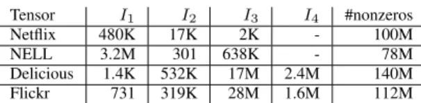
TABLE I: Tensors used in the experiments Tensor I1 I2 I3 I4 #nonzeros
Netflix 480K 17K 2K - 100M NELL 3.2M 301 638K - 78M Delicious 1.4K 532K 17M 2.4M 140M Flickr 731 319K 28M 1.6M 112M
be categorized into four classes: (i) toolboxes for Matlab and similar environments [24], [25], [26], [20], [27]; (ii) implemen-tations for shared memory systems [28], [29], [21], [30]; (iii) implementations based on MapReduce paradigm [12], [31]; (iv) implementations for distributed memory systems [11], [32], [16], [33]. The implementations in the first group are very useful tools that enable fast prototyping. Those in the second group and similar work are helpful when data fits into the memory of a single machine, which is nowadays large enough to accommodate tensors from many applications. Those in the third and fourth groups enable computations on tensors that do not fit into the memory of a single machine. The ones in the third group are not designed for high performance, as MapReduce paradigm is meant to perform multiple passes over out-of-core data and perform global communication shuffling the input data.
To the best of our knowledge, there is no high perfor-mance distributed memory implementation of algorithms for the sparse Tucker decomposition. Among the cited references above, HaTen2 [12] is a MapReduce based HOOI imple-mentation. Li et al. [21] investigate efficient shared memory execution of tensor times matrix products and as a future work mention how this can be used to perform intra-node TTM computations in a distributed memory setting. This work does not discuss other components of an HOOI implementation. Austin et al. [11] propose a distributed memory parallel implementation of HOOI for dense tensors. The challenges that are faced are very different from those faced in the sparse case, essentially due to all communications involving all processes, and memory accesses being regular in the dense case.
V. EXPERIMENTALRESULTS
We conducted our experiments on an IBM Blue Gene/Q cluster, which consists of 6 racks of 1024 nodes with each node having 16 GBs of memory and a 16-core IBM PowerPC A2 processor running at 1.6 GHz. We ran our experiments up to 256 nodes (4096 cores) where we achieved the maxi-mum scalability. Each core of PowerPC A2 can handle one arithmetic and memory operation simultaneously; therefore we assigned 32 threads per node (2 threads per core) to benefit from this. All codes we used in our benchmarks were compiled using the Clang C++ compiler (version 3.6.0) with IBM MPI wrapper using -O3 option for compiler optimizations, and linked against IBM ESSL library for LAPACK and BLAS rou-tines. Our code depends on PETSc and SLEPc (version 3.6.2) libraries for the distributed truncated SVD computations.
We experimented with four tensors that we formed from real world data whose properties are in Table I. Netflix tensor
hasuser×movie×timedimensions, which we formed from the data of the Netflix Prize competition [34]. In this tensor, the nonzeros correspond to the user reviews of movies, and review date extends the data to the third dimension. The values of the nonzeros are determined by the corresponding review scores given by the users. We obtained the NELL tensor from the Never Ending Language Learning (NELL) knowledge database of the “Read the Web” project [2], which con-sists of tuples of the form (entity, relation, entity) such as (‘Chopin’,‘plays musical instrument’,‘piano’). The nonzeros of this tensor correspond to these entries discovered by NELL from the web, and the values are set to be the “belief” scores given by the learning algorithms used in NELL. Delicious and Flickr are the datasets for the web-crawl of Delicious.com and Flickr.com during 2006 and 2007, which is formed by G¨orlitz et al. [35]. These datasets consist of tuples of the form (time×users×resources×tags); hence we naturally form 4-mode tensors out of these tuples.
Our parallel algorithms are independent from the partition-ing method. Therefore, we use two partitionpartition-ing methods to test their performance. The first partitioning method assigns the tasks uniformly at random to processes (for coarse-grain tasks we use a blocked variant), and the second one uses hypergraph partitioning tool PaToH [36]. The first method is fast, promises load balance, but it does not pay attention to the communication overhead. The second method achieves load balance, reduces communication, but is time consuming. Speedups using these two partitioning methods show the worst case behavior and the potential of the parallel algorithms, if one is willing to pay the preprocessing cost. In general, a good parallel algorithm should deliver good performance with the second partitioning method; but it should also enjoy acceptable speed up with the first partitioning method.
We used PaToH (version 3.2) with default options to parti-tion the hypergraphs. We created all partiparti-tions offline, and ran our experiments on these partitioned tensors on the cluster. We do not report timings for partitioning hypergraphs with PaToH, which is costly. Yet in most applications, the tensors from the real-world data are built incrementally and analyzed repetitively. In this scenario, a partition for the updated tensor can be formed by refining the partition of the previous tensor. Also, one can decompose a tensor multiple times with different ranks of approximation [37]. In these cases, the time spent in partitioning can be amortized across multiple runs.
To the best of our knowledge, HaTen2 [12] is the only par-allel implementation of HOOI (see Section IV). All reported parallel runtimes of HaTen2 [12] are larger than that of the sequential execution of MET algorithm [26], [20], and the sequential runtime of our method is less than that of MET. For example, on a random tensor of size 10K×10K×10K with 1M nonzeros, Tucker decomposition with five HOOI iterations took 87.2 seconds in MET and 11.3 seconds in our method (on a single core), including all preprocessing. This difference is expected as neither HaTen2 (which uses MapReduce) nor MET (which is a Matlab tool) are made for high performance; thus, we do not report further comparisons.
We set the ranks of approximation R1 =R2 =R3 = 10
for the 3-mode tensors, and R1 = R2 = R3 = R4 = 5
for the 4-mode tensors, which is a viable choice in data analysis applications [5], [6]. We then run the parallel HOOI for 5 iterations, and report the average time spent per HOOI iteration. The symbolic TTMc is expected take much less time than the HOOI iterations. For instance, in 256-way parallel execution of Algorithm 4 using the fine-grain hypergraph partitioning for 5 iterations, symbolic TTMc took 14%, 12%, 19%, and 5% of the total execution time for Delicious, Flickr, Netflix, and NELL tensors, respectively. In general, HOOI is expected to run for more iterations; so this cost is expected to become less important. In addition, finding a good Tucker approximation of a tensor typically involves executing HOOI algorithm with various ranks [37]; symbolic TTMc can be computed once and used for all these executions.
A. Distributed memory results
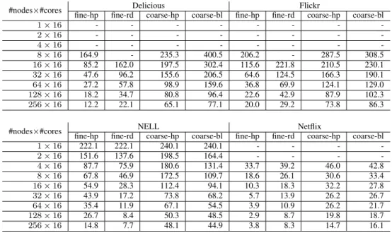
In Table II, we give the strong scalability results for our distributed memory parallel HOOI algorithm. We report the average time spent per iteration in Algorithm 4. For each tensor in our dataset, we report two results for fine-grain and coarse-grain parallel algorithms (with two different partition-ing methods). Those with the suffix “-hp” uses PaToH’s par-titionings; “fine-rd” refers to a random partitioning, whereas and “coarse-bl” corresponds to a contiguous block partitioning of tasks. We evaluate the algorithms up to 256 compute nodes where each node executes Algorithm 4 using 32 threads. Since the amount of memory per node of Blue Gene/Q is only 16GBs, some runs were not feasible. These missing runs are shown with “-” in Table II. In two tensors, using the fine-rd partition was feasible only after 16 nodes due to higher memory requirements for storing partial results (which is proportional to the communication cost).
We first observe in Table II that in all test cases our algorithm graciously scale up to 256 MPI ranks (or 4096 cores), except with the fine-hp partition on Netflix tensor, where we observe a slowdown at 256 nodes. On Delicious tensor, our parallel algorithm achieves 13.5x speedup using 256 nodes over the run on 8 nodes with the fine-hp partition. With the fine-rd partition, the algorithm also scales to 256 nodes, although it runs almost two times slower than fine-hp. This is expected, as fine-rd targets load balance but incurs more communication overhead. Similarly on Flickr, our parallel algorithm achieves 10.3x speedup using 256 nodes over its execution on 8 nodes with the fine-hp partition, and runs roughly twice as fast as the configuration with the fine-rd partition. Unfortunately, with Delicious, Flickr, and Netflix datasets, we were not able to get the sequential and shared memory parallel timings on a single node due to data not fitting into the memory; hence we cannot provide overall speedup results over the sequential execution. For those results, we refer the reader to a technical report [38], where we present speedups up to 742x on a different architecture with more memory. On NELL tensor, we managed to get runs on a single node. Using the fine-rd partition using 256 nodes (4096 cores),
TABLE II: Time spent per iteration (in seconds) for our distributed memory parallel HOOI using two threads per core with different partitions. Missing results are due to small amount of memory in BlueGene/Q nodes.
#nodes×#cores Delicious Flickr
fine-hp fine-rd coarse-hp coarse-bl fine-hp fine-rd coarse-hp coarse-bl
1×16 - - - -2×16 - - - -4×16 - - - -8×16 164.9 - 235.3 400.5 206.2 - 287.5 308.5 16×16 85.2 162.0 197.5 302.4 115.6 221.8 210.5 230.1 32×16 47.6 96.2 155.6 206.5 64.6 124.5 166.3 190.1 64×16 27.2 57.8 98.9 159.6 36.8 69.9 124.1 129.0 128×16 18.2 34.7 80.8 96.4 22.6 42.9 87.9 102.3 256×16 12.2 22.1 65.1 77.1 20.0 29.2 73.8 86.3
#nodes×#cores NELL Netflix
fine-hp fine-rd coarse-hp coarse-bl fine-hp fine-rd coarse-hp coarse-bl
1×16 222.1 222.1 240.1 240.1 - - - -2×16 151.6 137.6 198.5 164.4 - - - -4×16 87.7 75.9 180.6 131.4 33.7 39.2 46.0 42.8 8×16 67.8 46.9 172.5 109.7 18.6 26.1 30.6 33.4 16×16 54.9 28.3 112.4 94.1 10.3 18.3 32.2 27.8 32×16 43.9 17.2 73.8 68.2 5.7 13.9 26.2 26.7 64×16 35.4 11.9 67.1 54.5 3.9 10.9 26.2 21.7 128×16 26.7 8.4 50.3 48.5 2.9 8.7 19.8 18.7 256×16 14.8 7.7 48.1 44.9 3.8 8.3 14.7 16.1
we obtained 280x speedup over the sequential execution. This translates into 29x speedup over the execution on a single node. Yet, unlike other three tensors, on this data the fine-hp partition lead to slower execution than the fine-rd partition. We analyzed the underlying reason for this result on 256 MPI ranks and saw that themaximumcommunication volume per process for with the fine-hp partition in the dominant dimension was 543K in contrast to 366K in the fine-rd partition. Here, this entailed a large overhead that could not be compensated by the reduction in the total communication volume (20M vs 94M).
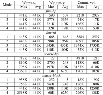
In Table III, we give the computation and communication requirements of one HOOI iteration on the Flickr tensor with all partitionings for 256 MPI ranks (4096 cores). In this table, WT T M c andWT RSV D correspond to the computational load
of the TTMc and TRSVD steps of Algorithm 4 and Comm. vol. corresponds to the volume of send/receive communication incurred by different partitioning methods. We give both the average and the maximum values across all processes for all three metrics.
We observe in theWT T M c columns of Table III that TTMc
work per MPI-rank is always well balanced with the fine-grain partitions. This is owing to the finer granularity of tasks which allows perfect balance. On the other hand, with the coarse-grain formulation, the TTMc tasks are not well balanced, as some tasks might be significantly more costly than others. Particularly in the TTMc computation of the 4th dimension, we observe some computational imbalance of 436% and 471% using the coarse-hp and coarse-block partitions.
We realize in the WT RSV D columns of Table III that
the average TRSVD work WT RSV D given by the fine-hp
partition is only slightly higher than that given by the coarse-grain partitions, which introduce no overhead to the TRSVD
computation. Particularly, WT RSV D is dominant in the third
dimension, and the fine-hp partition results in the same total/average work (110K) as in the coarse-grain partitions. Using the random partition (fine-rd), however, the average WT RSV Dis drastically increased to 435K in the same
dimen-sion. Moreover, even though none of the partitioning methods explicitly try to establish load balance for WT RSV D, we
ob-serve that the obtained load balance is generally acceptable. In the computationally dominant third mode, the fine-hp partition leads to 100% load imbalance, whereas the fine-rd, coarse-hp, and coarse-block partitions lead to 25%, 79%, and 18%.
The last two columns of Table III show the maximum and the average communication volume per process. This involves the send and receive volumes at Lines 13 and 14 of Algorithm 4. Using the fine-hp and fine-rd partitions, the average communication volumes are 11K and 1735K, respectively. Recall that the average communication volume is proportional to the cutsize of the corresponding hypergraph partition, and the cutsize equals to the total redundancy in MxV and MTxV operations. That is why we observe higher WT RSV D value using the fine-rd partition. The maximum
communication volume per process also decreases to 166K with fine-hp partition, in comparison to 1744K using fine-rd partition. Our final observation is that fine-hp partitions are more effective in reducing the communication volume than the coarse-hp partitions.
In Table IV, we provide the relative timings of TTMc, TRSVD, and the computation of the core tensor within an iteration of HOOI using the 256-way fine-hp partition. The TRSVD timings include the time spent in the communication of the vector entries in the MxV and MTxV operations, as the communication takes place within the PETSc calls. We see in Table II that on Netflix tensor with the fine-hp partition,
TABLE III: Statistics for the computation and communication requirements with different partitionings of Flickr in one HOOI iteration for 4096-way parallel run with 256 MPI ranks.
Mode WT T M c WT RSV D Comm. vol.
Max Avg Max Avg Max Avg
fine-hp 1 441K 441K 590 507 2218 2029 2 441K 441K 8778 5656 24K 17K 3 441K 441K 221K 110K 166K 11K 4 441K 441K 32K 19K 77K 53K fine-rd 1 443K 441K 668 648 5884 2597 2 443K 441K 98K 96K 409K 385K 3 443K 441K 545K 435K 1744K 1735K 4 443K 441K 110K 100K 432K 413K coarse-hp 1 718K 441K 22 3 4910 1213 2 810K 441K 2700 248 118K 66K 3 798K 441K 197K 110K 3187K 810K 4 2368K 441K 13K 6250 170K 102K coarse-block 1 958K 441K 252 3 18K 907 2 756K 441K 5401 248 126K 80K 3 441K 441K 130K 110K 3324K 1250K 4 2518K 441K 60K 6250 296K 138K
TABLE IV: Relative timings of TTMc, TRSVD, and core tensor computation steps within HOOI using 256-way fine-hp partition (in percentage)
Step Delicious Flickr NELL Netflix TTMc 75.6 64.6 71.2 27.7 TRSVD+comm 19.2 32.6 24.8 71.6 core+comm 5.2 2.8 4.0 0.7
we lose scalability at 256 nodes. Table IV shows that for this instance TRSVD step begins to dominate the timings, and the communication cost starts to prevent further scalability. Note that in this case, the increase in the communication cost and imbalance also affects the computational cost of the TRSVD step. This is because of the fact that for each communicated vector entry there is an associated unit of redundant work in the MxV and MTxV computations. We also realize in these results that the cost of forming the core tensorGwith a TTM followed by an AllReduce communication is negligible, as we expected. Finally, we inform that in all instances, TRSVD (as provided by SLEPc) converged in less than 5 iterations.
TABLE V: Time spent per iteration (in seconds) for shared memory parallel HOOI on node(s) with a 16-core processor. The number of MPI ranks used for each tensor is shown in the parentheses.
#threads Delicious (8) Flickr (8) NELL (1) Netflix (4) 1 1182.7 1055.8 2173.6 660.1 2 634.5 583.2 1146.3 330.8 4 361.1 354.5 616.4 167.6 8 227.5 241.6 354.1 87.3 16 173.2 201.0 252.7 48.7 32 164.9 206.2 222.7 33.7
B. Shared memory results
We evaluate the shared memory scalability of the distributed memory HOOI algorithm by varying the number of threads from 1 to 32, and using the minimum number of nodes possible. We needed 8, 8, 4, and 1 nodes to be able to execute the code on Delicious, Flickr, Netflix, and NELL, respectively, using the fine-hp partitions.
TTMc is a memory latency-bound operation; for each nonzero xi,j,k, the access to U1(i,:), U2(j,:), and U3(k,:)
likely results in a cache miss, due to the irregular pattern of nonzeros. Multi-threading is an effective way of hiding this latency; therefore it offers a great opportunity of acceleration through parallelism. However, the MxV and MTxV operations in the TRSVD step are memory bandwidth-bound due to the matrices being dense. Once the memory bandwidth is saturated, one may not expect a notable speedup with multi-threading (except in a NUMA architecture where each socket has an independent memory bandwidth; yet in this case the parallelism within a socket has the same issue). The TTMc operation count is proportional to the number of nonzeros, whereas the TRSVD cost is proportional to the number of rows of the matrix (or equivalently, the size of a dimension of the tensor).
As seen in Table V, we manage to improve the runtime using 32 threads for all tensors except Flickr. Using 32 threads, the speedups we obtain for Delicious and Flickr tensors are 7.2x and 5.1x, whereas on NELL and Netflix we get 9.8x and 20x, respectively. Delicious and Flickr tensors have very large third dimension of size 17M and 28M, whereas the largest dimensions of NELL and Netflix are of size 3.2M and 480K. Therefore, NELL and particularly Netflix have more latency-bound computations and provide more room for speedup, which explains the better speedup results in comparison to Delicious and Flickr tensors. Another interesting point is that on the Netflix tensor, using 16 threads we achieve 13.8x speedup over the single threaded execution. Increasing to 32 threads results in a superlinear speedup of 20x on 16 cores. We believe that this is mostly due to each core being able to execute two threads (one for memory and one for compute operations) simultaneously, which is particularly advantageous for latency-bound sparse irregular operations.
VI. CONCLUSION
We discussed an efficient parallelization of the alternating least squares-based Tucker decomposition algorithm (HOOI, also called Tucker-ALS) for sparse tensors in shared and distributed memory systems. We introduced a nonzero-based TTMc formulation, and proposed a shared-memory parallel HOOI with a preceding symbolic computation step that uses this formulation. We proposed a coarse and a fine-grain par-allel algorithm with their corresponding task definitions, and investigated the issues of load balance and communication cost reduction on different components of the the parallel algoritms. Gathering all these together, we achieved scalability up to 4096 cores using 256 MPI ranks on real world tensors with
an efficient hybrid OpenMP-MPI implementation within our high performance parallel sparse tensor library, HyperTensor. We finally note that the TTMc operation is used in other algorithms [39] for Tucker decomposition; therefore, proposed methods of parallelism can be used by those algorithms.
ACKNOWLEDGMENT
This work was performed using HPC resources from GENCI-[TGCC/CINES/IDRIS] (Grant 2016 - i2016067501).
REFERENCES
[1] T. G. Kolda and B. Bader, “The TOPHITS model for higher-order web link analysis,” inProceedings of Link Analysis, Counterterrorism and Security, 2006.
[2] A. Carlson, J. Betteridge, B. Kisiel, B. Settles, E. R. H. Jr., and T. M. Mitchell, “Toward an architecture for never-ending language learning,” inAAAI, vol. 5, 2010, p. 3.
[3] K. Bollacker, C. Evans, P. Paritosh, T. Sturge, and J. Taylor, “Free-base: A collaboratively created graph database for structuring human knowledge,” inProceedings of the 2008 ACM SIGMOD International Conference on Management of Data. New York, NY, USA: ACM, 2008, pp. 1247–1250.
[4] S. Rendle, B. M. Leandro, A. Nanopoulos, and L. Schmidt-Thieme, “Learning optimal ranking with tensor factorization for tag recom-mendation,” in Proceedings of the 15th ACM SIGKDD International Conference on Knowledge Discovery and Data Mining, ser. KDD ’09. New York, NY, USA: ACM, 2009, pp. 727–736.
[5] P. Symeonidis, A. Nanopoulos, and Y. Manolopoulos, “Tag recommen-dations based on tensor dimensionality reduction,” in Proceedings of the 2008 ACM Conference on Recommender Systems. New York, NY, USA: ACM, 2008, pp. 43–50.
[6] Y. Xu, L. Zhang, and W. Liu, “Cubic analysis of social bookmarking for personalized recommendation,” inFrontiers of WWW Research and Development-APWeb 2006. Springer, 2006, pp. 733–738.
[7] C. J. Appellof and E. R. Davidson, “Strategies for analyzing data from video fluorometric monitoring of liquid chromatographic effluents,”
Analytical Chemistry, vol. 53, no. 13, pp. 2053–2056, 1981.
[8] L. D. Lathauwer and B. D. Moor, “From matrix to tensor: Multilinear algebra and signal processing,” in Institute of Mathematics and Its Applications Conference Series, vol. 67, 1998, pp. 1–16.
[9] M. A. O. Vasilescu and D. Terzopoulos, “Multilinear analysis of image ensembles: TensorFaces,” inComputer Vision—ECCV 2002. Springer, 2002, pp. 447–460.
[10] K. Maruhashi, F. Guo, and C. Faloutsos, “MultiAspectForensics: Pattern mining on large-scale heterogeneous networks with tensor analysis,” in
International Conference on Advances in Social Networks Analysis and Mining (ASONAM), July 2011, pp. 203–210.
[11] W. Austin, G. Ballard, and T. G. Kolda, “Parallel tensor compression for large-scale scientific data,” arXiv, Tech. Rep., 2015.
[12] I. Jeon, E. E. Papalexakis, U. Kang, and C. Faloutsos, “Haten2: Billion-scale tensor decompositions,” inIEEE 31st International Conference on Data Engineering (ICDE), 2015, pp. 1047–1058.
[13] P. Comon, “Tensors: A brief introduction,” IEEE Signal Processing Magazine, vol. 31, no. 3, pp. 44–53, May 2014.
[14] T. G. Kolda and B. Bader, “Tensor decompositions and applications,”
SIAM Review, vol. 51, no. 3, pp. 455–500, 2009.
[15] L. D. Lathauwer, B. D. Moor, and J. Vandewalle, “On the best rank-1 and rank-(R1, R2, . . . , RN)approximation of higher-order tensors,”
SIAM Journal on Matrix Analysis and Applications, vol. 21, no. 4, pp. 1324–1342, 2000.
[16] O. Kaya and B. Uc¸ar, “Scalable sparse tensor decompositions in dis-tributed memory systems,” in Proceedings of the International Con-ference for High Performance Computing, Networking, Storage and Analysis. New York, NY, USA: ACM, 2015, pp. 77:1–77:11. [17] S. Balay, S. Abhyankar, M. F. Adams, J. Brown, P. Brune, K.
Buschel-man, L. Dalcin, V. Eijkhout, W. D. Gropp, D. Kaushik, M. G. Knepley, L. C. McInnes, K. Rupp, B. F. Smith, S. Zampini, and H. Zhang, “PETSc web page,” http://www.mcs.anl.gov/petsc, 2015.
[18] J. E. Roman, C. Campos, E. Romero, and A. Tomas, “SLEPc users manual,” D. Sistemes Inform`atics i Computaci´o, Universitat Polit`ecnica de Val`encia, Tech. Rep. DSIC-II/24/02 - Revision 3.6, 2015.
[19] L. D. Lathauwer, B. D. Moor, and J. Vandewalle, “A multilinear singular value decomposition,”SIAM Journal on Matrix Analysis and Applications, vol. 21, no. 4, pp. 1253–1278, 2000.
[20] T. G. Kolda and J. Sun, “Scalable tensor decompositions for multi-aspect data mining,” inICDM 2008: Proceedings of the 8th IEEE International Conference on Data Mining, Pisa, Italy, 2008, pp. 363–372.
[21] J. Li, C. Battaglino, I. Perros, J. Sun, and R. Vuduc, “An input-adaptive and in-place approach to dense tensor-times-matrix multiply,” in Proceedings of the International Conference for High Performance Computing, Networking, Storage and Analysis. Austin, Texas: ACM, New York, NY, USA, 2015, pp. 76:1–76:12.
[22] K. Kaya, F. H. Rouet, and B. Uc¸ar, “On partitioning problems with complex objectives,” inEuro-Par 2011: Parallel Processing Workshops. Springer Berlin / Heidelberg, 2012, vol. 7155, pp. 334–344.
[23] A. Pinar and B. Hendrickson, “Partitioning for complex objectives,” in
Proceedings of the 15th International Parallel & Distributed Processing Symposium (CDROM). Washington, DC, USA: IEEE Computer Society, 2001, p. 121.
[24] C. A. Andersson and R. Bro, “The N-way toolbox for MATLAB,”
Chemometrics and Intelligent Laboratory Systems, vol. 52, no. 1, pp. 1–4, 2000.
[25] B. W. Bader and T. G. Kolda, “Efficient MATLAB computations with sparse and factored tensors,” SIAM Journal on Scientific Computing, vol. 30, no. 1, pp. 205–231, December 2007.
[26] B. W. Bader, T. G. Koldaet al., “Matlab tensor toolbox version 2.6,” Available online, February 2015.
[27] E. E. Papalexakis, C. Faloutsos, and N. D. Sidiropoulos, “ParCube: Sparse parallelizable CANDECOMP-PARAFAC tensor decomposition,”
ACM Transactions on Knowledge Discovery from Data, vol. 10, no. 1, pp. 3:1–3:25, 2015.
[28] M. Baskaran, B. Meister, N. Vasilache, and R. Lethin, “Efficient and scalable computations with sparse tensors,” inIEEE Conference on High Performance Extreme Computing (HPEC), Sept 2012, pp. 1–6. [29] M. M. Baskaran, B. Meister, and R. Lethin, “Low-overhead
load-balanced scheduling for sparse tensor computations,” inIEEE Confer-ence on High Performance Extreme Computing (HPEC). Waltham, MA, USA: IEEE, Sep. 2014, pp. 1–6.
[30] S. Smith, N. Ravindran, N. D. Sidiropoulos, and G. Karypis, “SPLATT: Efficient and parallel sparse tensor-matrix multiplication,” in29th IEEE International Parallel & Distributed Processing Symposium. Hyder-abad, India: IEEE Computer Society, May 2015, pp. 61–70.
[31] U. Kang, E. Papalexakis, A. Harpale, and C. Faloutsos, “GigaTensor: Scaling tensor analysis up by 100 times - Algorithms and discoveries,” inProceedings of the 18th ACM SIGKDD International Conference on Knowledge Discovery and Data Mining. New York, NY, USA: ACM, 2012, pp. 316–324.
[32] J. H. Choi and S. V. N. Vishwanathan, “DFacTo: Distributed factor-ization of tensors,” in27th Advances in Neural Information Processing Systems, Montreal, Quebec, Canada, 2014, pp. 1296–1304.
[33] S. Smith and G. Karypis, “DMS: Distributed sparse tensor factorization with alternating least squares,” Department of Computer Science and Engineering, University of Minnesota, Tech. Rep. 15-007, May 2015. [34] J. Bennett and S. Lanning, “The netflix prize,” inProceedings of KDD
cup and workshop, vol. 2007, 2007, p. 35.
[35] O. G¨orlitz, S. Sizov, and S. Staab, “PINTS: Peer-to-peer infrastructure for tagging systems,” inProceedings of the 7th International Conference on Peer-to-Peer Systems. Berkeley, CA, USA: USENIX Association, 2008, p. 19.
[36] ¨U. V. C¸ ataly¨urek and C. Aykanat, PaToH: A Multilevel Hypergraph Partitioning Tool, Version 3.0, Bilkent University, Department of Com-puter Engineering, Ankara, 06533 Turkey. PaToH is available at http://bmi.osu.edu/˜umit/software.htm, 1999.
[37] H. A. L. Kiers and A. der Kinderen, “A fast method for choosing the numbers of components in Tucker3 analysis,” British Journal of Mathematical and Statistical Psychology, vol. 56, pp. 119–125, 2003. [38] O. Kaya and B. Uc¸ar, “High-performance parallel algorithms for the
Tucker decomposition of higher order sparse tensors,” Inria, Grenoble – Rhˆone-Alpes, Tech. Rep. RR-8801, Oct 2015.
[39] L. Eld´en and B. Savas, “A Newton–Grassmann method for computing the best multilinear rank-(r1, r2, r3)approximation of a tensor,”SIAM Journal on Matrix Analysis and Applications, vol. 31, no. 2, pp. 248– 271, 2009.