190
IJSOM
August 2014, Volume 1, Issue 2, pp. 190-215 ISSN-Print: 2383-1359
ISSN-Online: 2383-2525 www.ijsom.com
An Integrated Inventory Model with Controllable Lead time and Setup Cost
Reduction for Defective and Non-Defective Items
M. Vijayashreea∗, R. Uthayakumara
a
Department of Mathematics, The Gandhigram Rural Institute – Deemed University, Gandhigram - 624 302. Dindigul, Tamil Nadu, India
Abstract
In this paper, the study deals with the lead time and setup reduction problem in the vendor-purchaser integrated inventory model. The cost of capital (i.e., opportunity cost) is one of the key factors in making the inventory and investment decisions. Lead time is an important element in any inventory system. The proposed model is presents an integrated inventory model with controllable lead time with setup cost reduction for defective and non defective items under investment for quality improvement. In this analysis, the proposed model, we assumed that the setup cost and process quality is logarithmic function. Setup cost reduction for defective and non defective items, is the main focus for the proposed model. The objective of the proposed model is to minimize the total cost of both the vendor-purchaser. The mathematical model is derived to investigate the effects to the optimal decisions when investment strategies in setup cost reductions are adopted. This paper attempts to determine optimal order quantity, lead time, process quality and setup cost reduction for production system such that the total cost is minimized. A solution p0rocedure is developed to find the optimal solution and numerical examples are presented to illustrate the results of the proposed models.
191
Keywords: Integrated inventory model, Vendor-purchaser coordination, Lead time crashing
cost, Setup cost reduction for defective and non defective items.
1. Introduction
In modern production management, controllable lead time and setup cost reduction are keys to business success and have attracted considerable research attention. Setup cost reduction is one of the important production activities in an integrated inventory control. Setup time reduction in manufacturing operations is widely recognized to provide significant benefits in areas such as cost, agility and quality. Many techniques are available to improve setup time such as a revising setup procedure, modifying tooling for standardized locating and clamping, or introducing robotic change over equipment, to name a few. Each technique will provide a certain level of benefit, and has associated costs. Given that, the goal of the firm is to select the setup cost reduction techniques that will minimize their overall costs. In traditional economic order quantity (EOQ) and economic production quantity (EPQ) models, most of the literature treating inventory problem, either in deterministic or probability models, the stock out or setup cost are regarded as prescribed constants and equal at the optimum. In modern production management, controllable lead time and ordering cost reduction and setup cost reduction are keys to business success and have attracted considerable research attention. Ordering quantity, service level and business competitiveness can be shown to possibly be influenced directly or indirectly via lead-time and or ordering cost control. The integrated inventory models treat the ordering cost and setup cost /or lead time as constants. However, in some practical situations, lead time and ordering cost can be controlled and reduced in various ways. However, in practice, setup cost can be controlled and reduced through various efforts such as worker training, procedural change and specialized equipment acquisition. Through the Japanese experience of Just-in-Time (JIT) production, the advantages and benefits associated with efforts to reduce the setup cost can be clearly supposed. The Just-in-Time (JIT) system plays an important role in present supply chain management. One of the major tasks of maintaining the competitive advantages of JIT production is to compress the lead time needed to perform activities associated with delivering high-quality products to customers. In the dynamic, competitive environment, successful companies have devoted considerable attention to reducing inventory cost and lead time and improving quality simultaneously. In recent years, industries have devoted considerable attention to reducing
192
inventory cost. We have developed an integrated inventory model with controllable lead time with setup cost reduction for defective and non-defective items.
2. Literature Review
In recent years, most inventory problems have their focus on the integration between the vendor and the buyer. For the supply chain management, establishment of long term strategic partnerships between the buyer and the vendor is advantageous for the two parties regarding costs, and therefore profits since both parties, cooperate and share information with each other to achieve improved benefits. In Several researchers have shown that the buyer and the vendor can achieve their own minimum total cost, or increase their mutual benefit through strategic cooperation with each other. In the current supply chain management (SCM) environment, companies are using JIT production to gain and maintain a completive advantage. JIT requires a spirit of cooperation between the buyer and the vendor, and it has been shown that forming a partnership between the buyer and the vendor is helpful in achieving substantial benefits for both [Goyal (1992)]. In this complex environment, successful companies have devoted considerable attention to reducing inventory cost and improving quality simultaneously. The Japanese have successfully introduced the just-in-time (JIT) manufacturing philosophy which calls for small production quantities and low inventories. Small production quantities reduce rework and scrap and provide flexibility with frequent production runs. It is well known that setup costs/times must be reduced in order to reduce production quantities. Setup costs/times are costs/times that it takes to go from the production of the last good piece of a prior run to the first good piece of a new production run. The reduced setup cost can hence result in benefits such as less investment in inventory, improved quality, and flexibility [Hall (1983) and Schonberger (1982)]. This research focused on only one aspect of the advantage of reducing setup costs/times, namely reduced inventory related costs. In the classical economic order quantity (EOQ) models, the vendor’s and buyer’s inventory problems are treated in separately and the EOQ formula can give an optimal solution for them respectively. This independent decision behavior usually cannot assure that the two parties as a whole reach the optimal status. Therefore, during the past four decades, many researchers pay more attention on the problem of joint replenishment that minimizes the total relevant costs for the vendor and the buyer.
193
The integration between vendor and buyer for improving the performance of inventory control has received a great deal of attention to the integrated approach has been examined for years. Goyal (1976) is among the first researchers who analyzed an integrated inventory model for single vendor and single buyer system. The framework he proposed has encouraged many researchers to present various types of integrated inventory system. For instance, Banerjee (1986) assumed that the vendor manufactures at a finite rate and considered a joint economic lot-size model in which a vendor produces to order for a buyer on lot-for-lot basis. Goyal (1988) relaxed the lot-for-lot policy and suggested that vendor’s economic production quantity should be an integer multiple of buyer purchase quantity. As a result of using the approach suggested in Goyal’s (1988) model, significant reduction in inventory cost can be achieved. Later, numerous researchers [see Goyal (2000), Hoque (2006), Pandey (2007), Tang (2004), Teng (2011) and Tsou (2009)] addressed integrated production-distribution inventory models extending the ideal of Goyal (1988) under various assumptions.
Lead time reduction is another important production activity in an integrated inventory control. Lead time can be reduced by an additional crashing cost; In other words, lead time is controllable. According to Hsu et al. (2009), crashing cost could be expenditures on equipment improvement, information technology, order expedite, or special shipping and handling. By shortening lead time, buyers can lower the safety stock, reduce the out-of-stock loss, improve the customer service level and increase the competitive advantage of business. Therefore, lead time reduction has been one of the most offered themes for both researchers and practitioners. Lead time is another essential factor in any supply chain and inventory management system. It generally consists of numerous constituents, such as order preparation, supplier lead time, delivery and setup time. Controlling lead time properly and taking the optimal order quantity are very important in attaining the minimum total inventory cost. The issue of lead time reduction has received a lot of interest in recent years. Lead time reduction has numerous benefits including quickly filled customer orders and reducing the finished goods inventory level. Lead time management is a significant issue in production and operation management. In fact, lead time usually consists of the following components [Tersine (1994)]: order preparation, order transit, supplier lead time, delivery time, and setup time. In many practical situations, lead time can be reduced at an added crashing cost; in other words, it is controllable. By shortening the lead time, we can lower the safety stock, reduce
194
the stockout loss and improve the customer service level so as to gain competitive edges in business. The Japanese experience of using Just-in-Time (JIT) production showed that the benefits associated with lead time control are clear. Therefore, reducing lead time is both necessary and beneficial. Inventory models incorporating lead time as a decision variable
were developed by several researchers. Liao et al. (1991)first devised a probability inventory
model in which lead time was the unique decision variable. Ben-Daya et al. (1994) extended Liao et al. (1991) model by considering both lead time and order quantity as decision
variables. Later, some studies [Moon (1998), Ouyang (1999b), Ouyang (1999c), Ouyang
(2000) and Ouyang (1999d)] in the field of lead time reduction generalized Ben-Daya et al. (1994) model by allowing reorder point as one of the decision variables. Later, many researchers (see Glock (2012), Ho (2009), and Ouyang (2007)) investigated various integrated production-inventory models for lead time reduction in single-vendor single-buyer supply
chain. In the recent year, Glock (2012a) developed the joint economic lot size problem. And
also Glock (2012) developed lead time reduction strategies in a single-vendor- single buyer integrated inventory model with lot size-dependent lead time and stochastic demand. Hoque (2013) developed a vendor buyer integrated production inventory model with normal distribution of lead time.
The Just-in-Time (JIT) system has received a great deal of attention in the field of production /inventory management. From an inventory standpoint, the ultimate goal of JIT is to produce/order small lot-size and to reduce inventory level, which can be achieved by reducing setup cost. In the literature, many authors have presented the analytical models to discuss the effects of investing in reduce setup cost. The initial result in the development of the setup cost reduction model is that of Porteus (1985) who introduced the concept and developed a framework of investing in reducing setup cost on EOQ model. The framework has encourage many researchers, such as Keller et al. (1988), Narsi et al. (1990), Kim et al. (1992) and
Paknejad et al. (1987) to examine setup cost reduction. Then, Ouyang et al. (1999a)
investigated the influence of ordering cost reduction on modified continuous review inventory systems involving variable lead time with partial backorders. Later, Woo et al. (2001) developed an integrated inventory model for a single vendor and multiple buyers with ordering cost/setup cost reduction. Zhang (2007) extended Woo et al.’s (2001) model by relaxing the assumption that the cycle times for all buyers and the vendor are the same. Later,
195
some researchers [see Chang (2006), Coates (1996) and Kim et al. (1992)] addressed setup cost/ordering cost reduction inventory models under various assumptions.
Quality has been highly emphasized in modern production/inventory management systems. Also, it has been evidenced that the success of Just-In-Time (JIT) production is partly based on the belief that quality is a controllable factor, which can be improved through various efforts such as worker training and specialized equipment acquisition. In the classical
Economic Order Quantity (EOQ) model, the quality-related issue is often neglected; it
implicitly assumes that quality is fixed at an optimal level (i.e., all items are assumed with perfect quality) and not controllable. However, this may not be true. In a real production environment, we can often observe that there are defective items being produced. These defective items must be rejected, repaired, reworked, or, if they have reached the customer, refunded; and in all cases, substantial costs are incurred. Porteus (1986) and Rosenblatt et al. (1986) were the first to explicitly elaborate on the significant relationship between quality imperfection and lot size. Specifically, Porteus (1986) extended the EOQ model to include a situation where the production process is imperfect, and based on this model he further studied the effects of investment in quality improvement by introducing the additional investing options. Since Porteus (1987), several authors proposed the quality improvement models under various settings, see e.g. Keller et al. (1988), Hwang et al. (1993), Moon (1994), Hong et al. (1995) and Ouyang et al. (1999). Pan et al. (2002) have developed an integrated supplier-purchaser model focused on the benefit from lead time reduction. Pan et al. (2004) have developed an integrated inventory model involving deterministic variable lead time and quality improvement investment. The objective of this paper is to present the vendor-purchaser integrated production inventory model to reduce the setup cost for defective and non defective items under investment for quality improvement.
The remainder of this paper is organized as follows. Section 3 describes the notations and assumptions used throughout this paper. In section 4 Model formulations for two cases. Case 1 for non defective items with setup cost reduction in section 4.1. An efficient algorithm is developed to obtain the optimal solution for non defective items in section 4.2. Case 2 for defective items under investment for quality improvement with setup cost reduction in section 4.3. An efficient algorithm is developed to obtain the optimal solution for defective items under investment for quality improvement in section 4.4. An illustrative numerical example
196
has provided both defective and non defective items in section 5 to illustrate the results. Finally, we draw some conclusion in section 6.
3. Notations and Assumptions
To establish the mathematical model, the following notations and assumptions of the model are as follows
3.1. Notations
To develop the proposed model, the following notations are used
D Average demand per unit time on the purchaser
P Production rate of the vendor
Q Order quantity of the purchaser (Decision Variable)
A Purchaser’s ordering cost per order
S Vendor’s setup cost per set-up (Decision Variable)
0
S Original vendor’s setup cost for each production run.
L Length of lead time in weeks
v
C Unit production cost paid by the vendor p
C Unit purchase cost paid by the purchaserCv <Cp
m The number of deliveries of the product delivered from the vendor to the purchaser in
one production cycle, a positive integer (Decision Variable)
α Vendor’s fractional opportunity cost of capital per unit time. (e. g. interest rate)
g Vendor’s unit rework cost per defective item
) (S
I Capital investment required to achieve setup cost ,S 0<S ≤S0
) (θ
I Capital investment required to reduce the out-of-control probability from
θ
0to θδ Percentage decrease S per dollar increase in investmentI(S)
λ Percentage decrease θper dollar increase in investmentI(θ)
r
Annual inventory holding cost per dollar invested in stocks.θ Probability of the vendor’s production process that can go out-of-control. (Decision
Variable)
0
197 3.2. Assumptions
The assumptions made in the paper are as follows
1. The product is manufactured with a finite production rate P , andP>D.
2. The system consists of a single vendor and a single purchaser for a single commodity has
been considered.
3. Inventory is continuously reviewed. The purchaser places the order when the inventory
position reaches the reorder point R .
4. The reorder point R = the expected demand during lead time+ safety stock
( )
SS , and(
standarddeviationoflead timedemand)
×
=k
SS , that isR= DL+k
σ
L where k is asafety factor.
5. The demand X during lead time L follows a normal distribution with mean µLand
standard deviation
σ
L.6. The lead time L consists of n mutually independent components. The ith component has
a normal durationb minimum durationi, a and crashing cost per unit timei c . For i
convenience, we rearrangec such thati c1 <c2 <c3 <...<cn. The components of lead
time are crashed one at a time starting from the first component because it has the minimum unit crashing cost, and then the second component, and so on.
7. Let
∑
= = n i i o b L 1and Li be the length of lead time with components 1,2,3....,icrashed to
their minimum duration, and then Lican be expressed as
(
b a)
i n LL i
j j j o
i = −
∑
=1 − , =1,2,..., and the lead time crashing cost per cycle( )
(
)
(
)
[
1]
1 1 1 , , − − = − − + − ∈ =∑
i i i j j j j i i L L c b a L L L c LR . In addition, the length of lead time is
equal for all shipping cycles, and the lead time crashing costs occur in each shipping cycle. See Liao et al. (1991).
8. The relationship between lot size and quality is formulated as follows: while vendor is
producing a lot, the process can go out of control with a given probability θ each time another unit is produced. The process is assumed to be in control in the beginning of the production process. Once out of control, the process produces defective items and continues to do so until the entire lot is produced. (This assumption is in line with Porteus (1986)).
198
9. The extra costs incurred by the vendor will be fully transferred to the purchaser if
shortened lead time is requested.
10.Once the production process shifts to an out-of-control state, the shift cannot be detected
until the end of the production cycle, and the process continuous production and a fixed proportion of the produced items are defective.
11.All defective items produced are detected after the production cycle is over, and rework cost for defective items will be incurred.
12.We assume that the capital investment,I
( )
S , in reducing setup cost is given by alogarithmic function,
( )
= S S q S I ln 0 for 0<S ≤S0, where =δ
1 q and δ is percentagedecrease S per dollar increase in investment I(S).
13.We assume that capital investment,I(θ), in improving process quality (reducing
out-of-control probability for
θ
0toθ ) is given by a logarithmic function,( )
=
θ
θ
θ
0 1ln q I for 0 0<θ
≤θ
, where = λ 1 1q and λ is percentage decreaseθ per dollar increase in
investment I(θ).(This investment function has also been used in [Porteus (1986),
Keller(1988) and Hong (1993)].
14.Defective item rework cost per unit time: the expected number of defective items in a run
of size mQ with a given probabilityθ that the process can go out of control is
2 2 2
θ
Q m (see Porteus (1986) for detail derivation). Thus, the defective cost per unit time is given by2
θ
gmQD
.
4. Model formulation for both defective and non defective items
The purchaser places an order after every Q demand; therefore, for average cycle time of
D Q
,
the expected ordering and lead time crashing costs per unit can be given by
Q AD and
( )
Q L DRrespectively. Purchaser ordering cost per year =
Q DA
199
Purchaser lead time crashing cost per year = R
( )
LQ D
The expected net inventory level just before arrival of a procurement is the safety stock
DL R
s= − . The expected net inventory level immediately after arrival of procurement is
s
Q+ . Hence the average inventory over the cycle can be approximated by Q+s
2 , i.e. L k Q σ +
2 (Assumption 3), so the purchaser’s holding cost per unit time is
+k L Q rCp σ 2 .
Purchaser holding cost per year = k L rCp
Q + σ 2
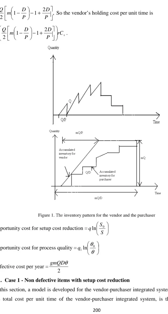
The vendor-purchaser integrated system is designed for a vendor’s production situation in which once the purchaser orders a lot size Q the purchaser begins production with a constant production rate P , and a finite number of units are added to inventory until the production run has been completed. The vendor produces the item in lot of size mQ in each production cycle of length
D mQ
, and the purchaser will receive the supply in m lots each of size Q . The
first lot of size Q is ready for deliveries after time
P Q
just after the start of the production,
and then the vendor continues making the delivery on average every
D Q
units of time until the
inventory level falls to zero ( see Fig 1). The total cost per unit time is given by
( )
mQSD
.
Vendor setup cost per year = S
mQ D
Vendor’s average inventory is evaluated as the difference of the vendor’s accumulated inventory and the purchase’s accumulated inventory. That is
D mQ m D Q P Q m D Q m P Q mQ − + + + − − − + (1 2 ... ( 1)) 2 ) 1 ( 2 2 2
200 , 2 1 1 2 + − − = P D P D m Q
So the vendor’s holding cost per unit time is
v rC P D P D m Q + − − = 1 1 2 2 .
Figure 1. The inventory pattern for the vendor and the purchaser
Opportunity cost for setup cost reduction =
S S q 0 ln
Opportunity cost for process quality =
θ
θ
0 1ln qDefective cost per year =
2
θ
gmQD
4.1. Case 1 - Non defective items with setup cost reduction
In this section, a model is developed for the vendor-purchaser integrated system to minimize the total cost per unit time of the vendor-purchaser integrated system, is the sum of the
201
ordering cost, holding cost and lead time crashing costs per unit time for the purchaser, investment cost required for setup cost reduction and holding costs per unit time for the vendor.
In addition, the target value of S is constrained on 0<S≤S0,As a result, in mathematical
symbolization. Therefore, the problem under study can be formulated as the following non linear programming model
(
Q L m S)
=TC , , , Ordering cost + vendor’s holding cost+ purchaser’s holding cost +
opportunity cost for setup cost+ purchaser’s lead time crashing cost
(
)
( )
+ + − − + + + = rCv rCp P D P D m Q S mQ D L R Q D Q DA S m L Q TC 1 1 2 2 , , , + + + S S q rCp L k Q 0 ln 2σ
α
( )
+ + − − + + + = Cv Cp P D P D m r Q L R m S A Q D 2 1 1 2 + + S S q L k rCp 0 lnα
σ
(1)Subject to 0<S ≤S0 where
α
is the annual fractional cost of capital investment (e.g., interest rate).To solve the above nonlinear programming problem, this study temporarily ignores the
constraint 0<S ≤S0and relaxes the integer requirement on m (the number of shipments from
the vendor to the purchaser during one production cycle). For fixed Q, Sand L∈
[
Li,Li−1]
,(
Q L m S)
TC , , , can be proved to be a convex function ofm. Consequently, the search for the
optimal delivery m*is reduced to find a local minimum.
Property 1. For fixed Q,Sand L∈
[
Li,Li−1]
, TC(
Q,L,S,m,)
is convex in m.Taking the first and second partial derivatives of TC(Q,L,m,S) with respect to m, we have
(
)
− + − = ∂ ∂ p D C Q Qm DA m m S L Q TC v 1 2 , , , 2 and(
, , ,)
2 0 3 2 = > ∂ ∂ Qm DA m m S L Q TC202
Therefore, TC
(
Q,L,S, m,)
is convex in m, for fixed Q,Sand L∈[
Li,Li−1]
. This completes theproof of Property 1. Next, the first partial derivatives of TC(Q,m,S)with respect to Q,Sand
[
, −1]
∈ Li LiL are taken for fixed m, respectively. This process yields
(
)
( )
+ + − − + + + − = ∂ ∂ p v C C P D P D m r L R m S A Q D Q m S L Q TC 2 1 1 2 , , , 2 (2)(
)
S q Qm D S m S L Q TC α − = ∂ ∂ , , , (3)(
)
2 1 2 1 , , , − + = ∂ ∂ L k rC c Q D L m S L Q TC p iσ
(4)Furthermore, for fixed
(
Q,S,m)
, TC(
Q, L, m, S)
is noted to be a concave function in[
− −1]
∈ Li Li L , because(
)
0 2 3 4 2 , , , < − − = ∂ ∂ L k C r L m S L Q TC pσ
(5)Hence, for fixed
(
Q,S,m)
the minimum total cost per unit time occurs at the end points of theinterval
[
Li−Li−1]
. On the other hand, by setting Equations. (2) - (3) equal to zero, we obtain( )
+ + − − + + = p v C C P D P D m r L R m S A D Q 2 1 1 2 (6) D qQm S =α
(7)For fixed m and L∈
[
Li −Li−1]
, by solving Equations (6)-(7), we can obtain the values ofS
Q, denote these value by
(
Q*, S*)
.The subsequent algorithm is proposed to find the optimal value of order quantity Q Lead ,
time ,L Opportunity cost of setup cost reduction ,S and number of deliveries m.
4.2. Algorithm in non defective items with setup cost reduction Step 1 set m=1 since mis integer.
Step 2 For each Li,i=1,2,3....n. Perform (2.1)-(2.6)
203 (2.2) SubstituteS into Eq. (6) evaluatesi1 Q . i1
(2.3) Utilizing Q determine i1 S from Eq. (7) s2
(2.4) Repeat (2.2)-(2.3) until no change occurs in the values of Q ,i Si
(2.5) Compare S′and S0
2.5.1. If Si <S0 then the solution found in step 1 is optimal for the given L . We i
denote the optimal solution by ( *, *).
i i S
Q then go to step (2.6).
2.5.2. If Si ≥So,then take Si* =S0 and utilize Eq. (6) to determine the new
*
i Q by
procedure similar to the one in (2.2). The result is denoted by
(
Qi*Si*)
.2.5.3. Utilize Eq. (1) to calculate the correspondingTC
(
Qi,Si ,Li,m)
* *
. Then go to step (3).
Step 3 Find min=1,2,3....nTC
(
Qi*,Si*,Li,m)
.Let TC
(
Q*(m),S(*m),L*(m),m*(m))
=min=1,2,3....n TC(
Qi*,Ss*,Li,m)
, then TC(
Q(*m),S(*m),L(m))
.is theoptimal solution for fixed m.
Step 4 Set m=m+1, repeat Step (2) – step (3) to get TC(Q(*m),S(*m),L*(m),m).
Step 5 If
(
, , ,)
.(
(* ), (* ), *( ), 1)
* ) ( * ) ( * ) ( S L m ≥TC Q S L m+ QTC m m m m m m , then go to step 4, otherwise go
to step 6.
Step 6 SetTC
(
Q*,S*,L*,m*)
=TC(
Q(*m+1),S(*m+1),L*(m+1),m+1)
, then TC(
Q*Ss*,L*,m*)
is theoptimal solution.
4.3.
Case 2- Defective items under investment for quality improvement with setup cost
reductionIn this section, a model is developed for the vendor-purchaser integrated system to minimize the total cost per unit time of the vendor-purchaser integrated system, it is the sum of the ordering cost, holding cost, and lead time crashing costs per unit time for the purchaser, investment cost required for setup cost reduction, investment cost required for quality improvement and holding costs per unit time for the vendor.
204
In addition, the target value of S,θ is constrained on 0<S≤S0, 0<
θ
≤θ
0.As a result, in mathematical symbolization. Therefore, the problem under study can be formulated as the following non linear programming model(
Q,L,m, S,θ
)
=TC Ordering cost + vendor’s holding cost+ purchaser’s holding cost +
opportunity cost for setup cost + Purchaser’s lead time crashing cost+ opportunity cost for process quality +defective cost
(
)
( )
v k L rCp Q P D P D m Q rc S mQ D L R Q D Q DA S m L Q TC + + + − − + + + =σ
θ
2 2 1 1 2 , , , , + + +θ
θ
α
θ
α
0 1 0 ln 2 ln gmQD q S S q( )
+ + + − − + + + = rC rC gmDθ
P D P D m Q L R m S A Q D p v 2 1 1 2 + + +θ
θ
α
α
σ
0 1 0 ln ln q S S q L k rCp (8)Subject to 0<S≤S0 ,0<
θ
≤θ
0.whereα
is the annual fractional cost of capital investment (e.g., interest rate).To solve the above nonlinear programming problem, this study temporarily ignores the constraint0< S≤S0,0<
θ
≤θ
0and relaxes the integer requirement on m (the number of deliveries from the vendor to the purchaser during one production cycle). For fixed Q, S,θ and L∈[
Li,Li−1]
, TC(
Q,L,m,S,θ
)
can be proved to be a convex function of m.Consequently, the search for the optimal deliveries *
m is reduced to find a local minimum.
Property 2. For fixed Q, S,θ and L∈
[
Li,Li−1]
, TC(
Q,L, S,m)
is convex in m.Taking the first and second partial derivatives of TC(Q,θ,m,S) with respect to m, we have + − + − = ∂ ∂
θ
θ
gD P D C Q Qm DS m L S m Q TC v 1 2 ) , , , , ( 2 0 2 ) , , , ( 3 2 2 > = ∂ ∂ Qm DS m S m Q TCθ
205
Therefore, TC
(
Q,L,Sθ
,m,)
is convex in m, for fixed Q,θ, Sand L∈[
Li,Li−1]
. Thiscompletes the proof of Property 2. Next, the first partial derivatives of TC(Q,θ,m,S)with respect to Q, S,θ and L∈
[
Li,Li−1]
are taken for fixed m, respectively. This process yields( )
+ + − = ∂ ∂ L R m S A Q D Q L S m Q TC 2 ) , , , , (θ
+ + + − − + rC rC gmDθ
P D P D m 1 1 2 v p 2 1 (9)θ
α
θ
θ
1 2 ) , , , , (Q m S L QgmD q TC − = ∂ ∂ (10) S q Qm D S L S m Q TCθ
= −α
∂ ∂ ( , , , , ) (11) 2 1 2 1 ) , , , , ( − + = ∂ ∂ L k rC c Q D L L S m Q TC p iσ
θ
(12) Furthermore, for fixed(
Q,S,θ,m)
, TC(
Q, L, S,θ,m,)
is noted to be a concave function in[
− −1]
∈ Li Li L , because(
)
0 2 3 4 2 , , , < − − = ∂ ∂ L k C r L m S L Q TC pσ
(13)Hence, for fixed
(
Q S,θ,m)
the minimum total cost per unit time occurs at the end points ofthe interval L∈
[
Li −Li−1]
. On the other hand, by setting Equations. (9) - (11) equal to zero, we obtain( )
θ
gmD rC P D P D m rC L R m S A D Q p v + + + − − + + = 2 1 1 2 (14) D qQm S =α
(15) gmDQ q1 2α θ = (16)For fixed mandL∈
[
Li −Li−1]
, by solving Equations (14)-(16), we can obtain the values of θ, , S
206
The subsequent algorithm is proposed to find the optimal value of order quantity Q Lead ,
time ,L opportunity cost of setup cost reduction ,S opportunity cost for process quality ,θ
and number of deliveries m.
4.4. Algorithm in defective items under investment for quality improvement and setup cost reduction
Step 1 set m=1 since mis integer.
Step 2 For eachLi,i=1,2,3....n. Perform (2.1)-(2.5.6)
2.1 Start with
θ
i1 =θ
0 ,Si1 =S0.2.2 Substitute
θ
i1,vi1into Eq. (14) which evaluatesQ . i12.3 Utilizing Q determines i1 S and i2
θ
i2 from Eq. (15) and (16).2.4 Repeat (2.2)-(2.3) until no change occurs in the values of Qi,Si,
θ
i2.5 Compare
θ
′andθ
0,andS′andS0respectively.2.5.1 If S′<S0 and
θ
′<θ
0, then the current solution is optimal for the given L .We idenote the optimal solution by (Qi*,θi*,Si*). If (Qi*,θi*,Si*).=(Qi',θi',Si'), then go to step (2.5.6), otherwise go to step (2.5.2).
2.5.2 If Si* <S0 and
θ
i* ≥θ
0,go to step (2.5.3). If Si* ≥S0andθ
i* <θ
0,go to step(2.5.4). If * ≥ 0 and
θ
* ≥θ
0,i i S
S then go to step (2.5.5).
2.5.3 Let θi* =θi and utilize Eq. (14), and (15) to determine the new (Qi′,Si′)by a procedure similar to the one in Step 2, the result is denoted by (Qˆi,θˆi).If Sˆi <S0 then the optimal solution is obtained, i.e., if (Qi*,θi*,Si*).= (Qˆi,θo,Sˆi). then go to step (2.5.6), otherwise go to step (2.5.3.1).
2.5.3.1 Let Si* =S0 and utilize Eq. (14) to determine the newQi′, then go to step
(2.5.6).
2.5.4 let Si* =S0and utilize Eq. (14), and (16) to determine the new (Qi′,
θ
i′)by a procedure similar to the one in Step 2, the result is denoted by (Qi,Si).r r
If
θ
i <θ
0r
207
the optimal solution is obtained, i.e., if (Qi*,θi*,Si*).=(Qi,θ,S0).
r r
then go to step (2.5.6), otherwise go to step (2.5.4.1).
2.5.4.1. Let θi* =θ0and utilize Eq. (14) to determine the newQi′, then go to step (2.5.6).
2.5.5 Let * 0
S
Si = and 0 * θ
θi = , and utilize Eq. (14) to determine the new Qi′, then
go to step (2.5.6).
2.5.6 Utilize Eq. (8) to calculate the correspondingTC(Qi*,
θ
i*i,Si*,Li*,m). Then go to step (3).Step 3 Find min=1,2,3....nTC
(
Qi*,Si*,θ
i*,Li,m)
.Let TC
(
Q*(m),θ
(*m), S(*m)L*s(m),m*)
=min=1,2,3....n TC(
Qi*,θ
(*m),S(*m),Li,m)
, then(
Q(*m), (*m)S(*m),,L*(m))
TC
θ
is the optimal solution for fixed m.Step 4 Set m=m+1, repeat step (2) – step (3) to get TC
(
Q*(m),L*(m),θ
(*m),S(*m), m)
.Step 5 If
(
, , , ,)
(
, ( ), (* ) , * , 1)
* ) ( * ) ( * * ) ( ) ( * ) ( * ) ( + ≥TCQ L S m m S L Q TC m m m m m m m mθ
θ
, then go to step (6), otherwise go to step (4). Step 6 Set(
, , , ,)
.(
, , , (* 1), 1)
* ) 1 ( ) 1 ( * ) 1 ( * * * * ) ( ) ( * ) ( * ) ( m = Q + L + + S + m+ S L Q m m θ m m m m θ m m , then ) , , , , ( * * * * * m L SQ
θ
is the set of optimal solution.5. Numerical Examples for both defective and non defective items (i) Non defective items
Consider an inventory system with following characteristics D=1000unit/ year,
year, unit/ 3200 =
P A=$25/order, S0 =$400/set−up,Cp =$25/unit,I
( )
ln ,0 = S S q S , 3500 =
q Cv =$20/unit, r=0.2,α =0.1, k=2.33,σ =7unit/week and the lead time has
208
Table 1. Lead time data for the illustrative example
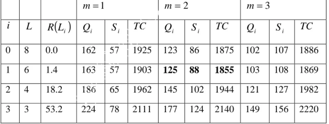
Applying the solution procedure of the proposed algorithm, the computational results are
demonstrated in table 2, number of deliveries m* =2, optimal lead time L* =4weeks,
optimal order quantity Q* =125 unit, Opportunity cost for setup cost reduction S* =$88,
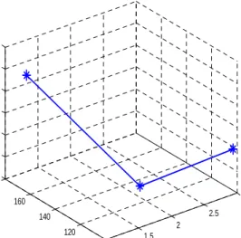
Total Cost TC =$1855. Pictorial representations and numerical analysis are presented to
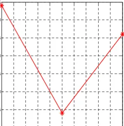
show the convexity of TC(Q,m,S, L) in figure (2) & (3).
Table 2. Summary of the solution procedure for the illustrative example for non defective items
1 = m m=2 m=3 i L R
( )
Li Qi Si TC Qi Si TC Qi Si TC 0 8 0.0 162 57 1925 123 86 1875 102 107 1886 1 6 1.4 163 57 1903 125 88 1855 103 108 1869 2 4 18.2 186 65 1962 145 102 1944 121 127 1982 3 3 53.2 224 78 2111 177 124 2140 149 156 2220 Lead time component i Normal duration(
days)
i b Minimum duration(
days)
i a Unit crashing cost(
$/days)
i c 1 20 6 0.1 2 20 6 1.2 3 16 9 5.0209
Figure 2. Pictorial representation for optimal solution for TC when L*=4 weeks, m=2, Q*=125
Figure 3. Pictorial representation for optimal solution
(ii) Defective items under investment for quality improvement with setup cost reduction
Consider an inventory system with following characteristicsD=1000unit/ year,
year, unit/ 3200 =
P A=$25/order, S0 =$400/set−up,Cp =$25/unit,I
( )
ln ,0 1 =
θ
θ
θ
q , 400 1 =q
θ
0 =0.0002, g =$15/perdefectiveunit,Cv =$20/unit, r=0.2,α =0.1, k =2.33,1 1.5 2 2.5 3 100 120 140 160 180 1850 1860 1870 1880 1890 1900 1910 Number of delivers (m) Qrder Quantity (Q) T o ta l C o s t (T C ) 1 1.2 1.4 1.6 1.8 2 2.2 2.4 2.6 2.8 3 1855 1860 1865 1870 1875 1880 1885 1890 1895 1900 1905 Number of delivers (m) T o ta l C o s t (T C )
210
( )
ln , I 0 = S S qS q=3500,σ =7unit/weekand the lead time has three components with data
shown on table 1.
Applying the solution procedure of the proposed algorithm, the computational results are
demonstrated in table 3, number of deliveries m* = 2 optimal lead time L* =4weeks,
optimal order quantity Q* =118unit, Opportunity cost for setup cost S* =$83,
Opportunity cost for process quality θ* =0.000022409, Total Cost TC =$1984. Pictorial
representations and numerical analysis are presented to show the convexity of ) , , , , (Q m S L TC θ in figure (4) & (5).
Table 3. Summary of the solution procedure for the illustrative example for defective items
1 = m m=2 m = 3 i L R
( )
Li Qi Si i θ TC Qi Si i θ TC Qi Si i θ TC 0 8 0.0 153 54 0.000034858 2036 117 86 0.000022792 2003 97 102 0.000018328 2023 1 6 1.4 154 54 0.000034632 2014 118 83 0.000022409 1984 99 104 0.000017957 2006 2 4 18.2 177 62 0.000030132 2079 138 97 0.000019324 2078 116 122 0.000015326 2126 3 3 53.2 216 76 0.000024691 2235 171 120 0.000015595 2282 145 152 0.000012261 2376Figure 4. Pictorial representation for optimal solution for TC when L*=4 weeks, m*=2 Q*=118
1 1.5 2 2.5 3 100 120 140 160 1980 1990 2000 2010 2020 Number of delivers(m) Qrder Quantity (Q) T o ta l C o s t (T C )
211
Figure 5. Pictorial representation for optimal solution
6. Conclusion
Reduction in setup cost, yield variability and lead time are important strategies in manufacturing system. The primary purpose of this paper is to present the vendor-purchaser integrated production inventory model under investment in quality improvements for defective and non defective items. Many companies have recognized the significance of lead time as a competitive weapon and have used lead time as a means of differentiating themselves in the market position. In the production environment, lead time is an important element in any inventory management system. The mathematical model is derived to investigate the effects of the best decisions when capital investment strategies in setup cost and investment for quality improvements are adopted. We developed an algorithm to minimize the total cost of the vendor-purchaser integrated system by simultaneously optimizing the order quantity, lead time, the number of deliveries, process quality, and setup cost reduction. In our model, the capital investment in process quality and setup cost reduction is assumed to be a logarithmic function. An iterative algorithm was devised to determine the optimal solution for optimal order quantity, process quality, lead time, setup cost reduction, and number of deliveries between the vendor and the purchaser. Furthermore, a numerical is given to illustrate the results for both defective and non defective items. Pictorial representation is also presented to illustrate the proposed model.
1 1.2 1.4 1.6 1.8 2 2.2 2.4 2.6 2.8 3 1980 1985 1990 1995 2000 2005 2010 2015 Number of delivers(m) T o ta l C o s t (T C )
212 Acknowledgement
The authors would like to acknowledge the Editor of the Journal and anonymous reviewer for
their support and helpful clarification in the revising the paper. The 1st author thankful to the
DST INSPIRE Senior Research Fellowship (SRF) Fellowship, Ministry of Science and Technology, Government of India, under the grant no. DST/INSPIRE Fellowship/AORC-IF/UPGRD/2014-15 dated 04.07.2014.
References
Banerjee, A. (1986). A joint economic-lot-size model for purchaser and vendor, Decision
Sciences, Vol.17, pp. 292-311.
Ben-Daya, M., and Raouf, A. (1994). Inventory models involving lead time as decision variable, Journal of the Operational Research Society, Vol. 45, pp.579-582.
Chang, H.C., Ouyang, L.Y., Wu, K.S. and Ho, C.H. (2006). Integrated vendor- buyer cooperative inventory models with controllable lead time and ordering cost reduction,
European Journal of Operational Research, Vol. 170, pp.481-495.
Coates, E.R. (1996). Manufacturing setup cost reduction, Computers and Industrial
Engineering, Vol. 31, pp. 111-114.
Glock C.H. (2012). Lead time reduction strategies in a single vendor-single buyer integrated inventory model with lot size-dependent lead time and stochastic demand. International
Journal of Production Economics, Vol. 136, pp. 37-44.
Glock C.H. (2012a). The joint economic lot size problem: A review. International Journal of
Production Economics, Vol. 135, pp. 671-686.
Goyal, S.K. (1976). An integrated inventory model for a single supplier single customer problem, International Journal of Production Research, Vol.15, pp.107-111.
Goyal, S.K. (1988). A joint economic-lot-size model for purchaser and vendor: A comment,
Decision Sciences, Vol.19, pp.236-241.
Goyal, S.K. and Nebebe, F. (2000). Determination of economic production-shipment policy for a single-vendor single-buyer system, European Journal of Operations Research, Vol. 121, pp. 175-178.
Goyal, S.K. and Srinivasan, G. (1992). The individually responsible and rational decision approach to economic lot sizes for one vendor and many purchasers: a comment, Decision
213
Hall, R.W., zero Inventories, Dow Jones Irwin, Homewood, IL, 1983.
Ho, C.H. (2009). A minimax distribution free procedure for an integrated inventory model with defective goods and stochastic lead time demand, International Journal of Information
and Management Sciences, Vol.20, pp.161-171.
Hong, J.D. and Hayya, J.C. (1995). Joint investment in quality improvement and setup reduction, Computers and Operations Research, Vol. 22, pp. 567-574.
Hoque, M.A. (2013). A vendor-buyer integrated production inventory model with normal distribution of lead time. International Journal of Production Economics, Vol. 144, pp.409-417.
Hoque, M.A. and Goyal, S.K. (2006). A heuristic solution procedure for an integrated inventory system under controllable lead-time with equal or unequal size batch shipments between a vendor and a buyer, International Journal of Production Economics, Vol. 102, pp. 217-225.
Hsu, S.L. and Lee, C.C. (2009). Replenishment and lead time decisions in manufacturer retailer chains, Transportation Research Part E, Vol.45, pp. 398-408.
Hwang, H., Kim, D.B. and Kim, Y.D. (1993). Multiproduct economic lot size models with investments costs for setup reduction and quality improvement, International Journal of
Production Research, Vol. 31, pp. 691-703.
Keller, G. and Noori, H. (1988). Impact of investing in quality improvement on the lot size model, Omega, Vol. 15, pp. 595-601.
Kim, K.L., Hayya, J.C. and Hong, J.D. (1992). Setup reduction in economic production quantity model, Decision Science, Vol. 23, pp. 500-508.
Liao, C.J., and Shyu, C.H. (1991). An analytical determination of lead time with normal demand, International Journal of Operations & Production Management, Vol.11, pp.72-78. Moon, I. (1994). Multiproduct economic lot size models with investments costs for setup reduction and quality improvement: Review and extensions, International Journal of
Production Research, Vol. 32, pp. 2795-2801.
Moon,I., and Choi,S. (1998). A note on lead time and distributional assumptions in continuous review inventory models, Computers & Operations Research, Vol. 25, pp. 1007-1012.
214
Nasri, F., Affisco, J.F. and Paknejad, M.T. (1990). Setup cost reduction in an inventory model with finite range stochastic lead times, International Journal of Production Research, Vol. 28, pp. 199-212.
Ouyang, L.Y. and Chang, H.C. (1999). Impact of investing in quality improvement on (Q, r, L) model involving the imperfect production process, Production Planning Control, Vol. 11, pp.598-607.
Ouyang, L.Y., Chen, C.K. and Chang, H.C. (1999a). Lead time and ordering cost reductions
in continuous review inventory systems with partial backorders, Journal of the Operational
Research Society, Vol. 50, pp. 1272-1279.
Ouyang, L.Y., Wu, K.S. and Ho, C.H. (2004). Integrated vendor-buyer cooperative models with stochastic demand in controllable lead time, International Journal of Production
Economics, Vol. 92, pp.255-266.
Ouyang, L.Y., Wu, K.S. and Ho, C.H. (2007). An integrated vendor buyer inventory model with quality improvement and lead time reduction, International Journal of Production
Economics, 108, 349-358.
Ouyang, L.Y., and Chuang, B.R. (1999b). (Q, R, L,) inventory model involving quantity
discounts and a stochastic backorder rate, Production Planning & Control, Vol. 10, pp. 426-433.
Ouyang, L.Y., and Chuang, B.R. (1999c). A minimax distribution free procedure for
stochastic inventory models with a random backorder rate, Journal of the Operations
Research Society of Japan, Vol. 42, pp.342-351.
Ouyang, L.Y., and Chuang, B.R. (2000). Stochastic inventory models involving variable lead time with a service level constraint, Yugoslav Journal of Operations Research, Vol. 10, pp.81-98
Ouyang, L.Y., Chuang, B.R., and Wu, K.S. (1999d). Optimal inventory policies involving
variable lead time with defective items, Journal of the Operational Research Society of India, Vol.36, pp. 374-389.
Paknejad, M. J. and Affisco, J. F. (1987). The effect of investment in new technology on optimal batch quantity, Proceedings of the Northeast Decision Sciences Institute, DSI, RI,
215
Pan, J.C.H. and Yang, J.S. (2004). Just-in-time: an integrated inventory model involving deterministic variable lead time and quality improvement investment, International Journal of
Production Research, Vol. 42, pp. 853-863.
Pan, J.C.H. and Yang, J.S.A. (2002). Study of an integrated inventory with controllable lead time, International Journal of Production Research, Vol. 40, pp. 1263-1273.
Pandey, A., Masin, M. and Prabhu, V. (2007). Adaptive logistic controller for integrated design of distributed supply chains, Journal of Manufacturing Systems, Vol.26, pp. 108-115. Porteus, E.L. (1985). Investing in reduced setups in the EOQ model, Management Sciences, Vol. 31, pp. 998-1010.
Porteus, E.L. (1986). Optimal lot sizing process quality improvement and setup cost reduction, Operations Research, Vol. 34, pp.137-144.
Rosenblatt, M.J. and Lee, H.L. (1986). Economic production cycles with imperfect production processes, IIE Transactions, Vol.18, pp. 48-55.
Schonberger, R. (1982). Japanese Manufacturing Techniques, the Free, New York.
Tang, J., Yung, K.L. and Ip, A. W.H. (2004). Heuristics-based integrated decisions for logistics network systems, Journal of Manufacturing Systems, Vol.23, pp.1-13.
Teng, J.T., Crdenas, B.L.E. and Lou, K.R. (2011). The economic lot-size of the integrated vendor-buyer inventory system derived without derivatives: a simple derivation, Applied
Mathematics and Computation, Vol. 217, pp. 5972-5977.
Tersine, R. (1994). Principle of Inventory and Material Management, Fourth Edition. Prentice-Hall, USA.
Tsou, C.S., Fang, H.H., Lo, H.C., Huang, C.H. (2009). A study of cooperative advertisings in a manufacturer-retailer supply chain, International Journal of Information and Management
Sciences, Vol. 20, pp. 15-26.
Woo, Y.Y., Hsu, S.L. and Wu, S.H. (2001). An integrated inventory model for a single vendor and multiple buyers with ordering cost reduction, International Journal of Production
Economics, Vol. 73, pp. 203-215.
Zhang, T., Liang, L., Yu, Y. and Yan, Y. (2007). An integrated vendor-managed inventory model for a two-echelon system with order cost reduction, International Journal of